URBAN ACTIVITY PATTERNS MINING IN WI-FI ACCESS POINT LOGS
GUILHEM POUCIN
DÉPARTEMENT DES GÉNIES CIVILS, GÉOLOGIQUE ET DES MINES ÉCOLE POLYTECHNIQUE DE MONTRÉAL
MÉMOIRE PRÉSENTÉ EN VUE DE L’OBTENTION DU DIPLÔME DE MAÎTRISE ÈS SCIENCES APPLIQUÉES
(GÉNIE CIVIL) MARS 2017
c
ÉCOLE POLYTECHNIQUE DE MONTRÉAL
Ce mémoire intitulé :
URBAN ACTIVITY PATTERNS MINING IN WI-FI ACCESS POINT LOGS
présenté par : POUCIN Guilhem
en vue de l’obtention du diplôme de : Maîtrise ès sciences appliquées a été dûment accepté par le jury d’examen constitué de :
M. BILODEAU Guillaume-Alexandre, Ph. D., président M. FAROOQ Bilal, Ph. D., membre et directeur de recherche
M. PATTERSON Zachary, Ph. D., membre et codirecteur de recherche M. YU Jia Yuan, Ph. D., membre
DEDICATION
A toutes les personnes dont j’ai croisé le chemin, A ma famille et mes amis aux quatres coins du monde, A la princesse slave et au boulanger philosophe, C’était cool de vous voir..
AKNWOLEDGMENTS
I want to thank my supervisor Bilal Farooq and Zachary Patterson for their support during this experience. Their patience and knowledge allowed me to complete this modest work and learn on a personal point of vue.
This research would not have been possible without the help of a number of people and institutions. First, we would like to thank Mike Babin, Myung Hong and Lichuan Yang of IITS at Concordia University for extracting the data from Wi-Fi network. Special thanks to Adam Taka, a Ph.D. student at LITrans, Polytechnique for developing the MAC address anonymization script for the preprocessing of Wi-Fi network logs. This research has been funded by FRQNT-New Researcher grant.
Finally, I want to thank my friends and family for their unconditional support during this experience far from my native home.
RÉSUMÉ
Aujourd’hui la grande majorité des données sont basée sur des enquêtes ou des études ap-pliquées à des échantillons définis de la population. De plus les méthodes traditionnelles de collecte de données en termes de coûts ainsi que de temps tout en ne garantissant pas la représentativité des observations du fait du biais d’échantillonages et de la relative fiabilité des répondants.
La disponibilité grandissantes de bases de données collectées passivements couplé à la forte pénétration des smartphones ont ouvert des perspectives intéressantes concernant la collecte et le traitement automatisé de données de mobilité.
L’utilisation de données provenant de réseaux omniprésents tels que les réseaux de commu-nication téléphoniques ou Wi-Fi est un domain en cours de développement. Des cas d’étude ont été déeveloppés à differentes éechelles, qu’il s’agisse d’un batîment, d’un campus ou d’une ville. Des études récentes tentent de fusionner ces données avec d’autres sources dìnformation, ce processus se révélant compliqué, spécialement dans les cas désagrégés.
La Media adress Control (adresse MAC) est un identifiant unique propre à chaque appareil permettant de les identifier au sein dùn réseau. Cette adresse reste fixe à vie pour chaque appareil est permet ainsi de retracer leurs historiques de connexion au sein des bases de données Wi-FI. En associant les positions des bornes d’accées Wi-FI, généralement fixes, ont peut donc retracer les positions successives de l’utilisatuer a lorsque son appareil est connecté au réseau.
Nous proposons au travers de ce travail de classifier les activitées réalisées par les utilisateurs du réseau Wi-Fi, à une petite échelle (batîment) sans conaissance préalable de la géographie des infrastructures (localisation spatiale des points d’accés). Pour cela , nous nous appuyons sur des algorithmes d’extraction de données en utilisant la méthodologie des K-moyennes guidées par analyse en composantes principales. Les résultats obtenus, générés l’échelle tem-porelle d’un jours sont ensuite mis en perspective à l’échelle de la semaine. Nous utilisons finalement les données géospatiales afin de valider les résultats obtenus.
Travaux antérieurs
L’études des données issues des données de communications tels que les réseaux téléphniques, le GPS ou les réseaux de Wi-Fi à reçu une attention grandissante durant les dernières dé-cénies. L’étude de la mobilité des utilisatuer se fait au travers de l’aquisition de leurs trace
qui peuvent être obtenues de trois manières différentes : la surveillance de leurs localisation, de leurs communications ou encore de leurs contact. LA surveillance de la localisation, ma-joritairement effectuées au travers u GPS consiste à enregistrer les positions successives de l’appareil grâce à son propre outils de géolocalisation : cette méthode est considérée comme centrées sur l’appareil. La surveillance des communications consite à reconstituer l’historiques des connectiosn effectiuées par l’appareil et des points d’accés concernés : cette méthode est considérée comme centrées sur le réseau.Enfin, la surveillance des contacts, encore en cours de développement consiste à enregistrer l’ensemble des appareils rencontrées par l’utilisateur. Si les données collectées au travers de la surveillance des communications des appareils pré-sente l’avantage de fournir une base de données contenant un écahntillon important de la population à moindre coût, certains probles doivent être surmontés. Le première obstacle découle de la nécessité d’anonimisation de ces bases de données pour des questions de sé-curité de la vie privée : la base de données ne contient généralement aucune données socio-démographiques concernant les utilisateurs. Il devient alors difficile de caractériser l’échan-tillon de population étudié, notamment dû a la variation du nombre d’appareil possédés par chaques utilisateurs. Ensuite, une partie des compotements des utilisateurs n’est pas observable, à partir du moment ou l’utilisateur n’est plus connecté au réseau : différencier l’absence du batiment de l’extinction de l’appareil est compliqué. Enfin, l’absence de mesure de position géographique peut creer l’apparition d’erreur ou bruit connu sous le non d’effet Ping Pong, avec l’apparitions d’enregistrement non représentatif d’événement réels.
Un travail considérable a été effectué dans le domaine du traitement des données de connec-tions Wi-FI. A l’origine destiné l’optimisation du design et de l’efficacité des réseaux de Wi-FI dans les lieux à forte fréquentation, le doamine d’application s’éetend aujourd’hui à l’étude de la mobilité des usagers. Divers process de pré traitement de ces données ont été proposés, notamment concernant la diminution de l’impact de l’effet Ping Pong, au travers de processus d’aggrégation.
Un travail a été effectué, proposant de classer les différents types d’activité réalisés autours des points d’accés WI-FI. En décomposant en élément propres la matrice de l’évolution du nombre d’usagers connectés en fonction du temps, puis en applicant l’algorithme des K moyennes, 5 familles d’activités sont générées. Nous proposons dans notre travail une alternative à la décomposition en éléments propre, permettant en autre d’incorporer les notions de temps de connections pour les utilisatuers. De plus, à l’instar de l’étude mentionnée, nous n’utilisons aucun données géospatiales lors de la calibration de l’algorithme, afin de limiter les données nécessaires.
Données et et traitement des erreurs
Notre méthodologie s’appuie sur le cas d’étude de l’université de Concordia (Montréal, Ca-nada). La base de donnée concerne les connections au réseaux Wi-Fi de l’université sur une semaine, enregistée en février 2015. La base comporte environs 1.7 millions de connections effectuées par plus de 60.5000 appareils intelligents. Les appareils sont identifiés à l’aide de leurs MAC adress, permettant ansi de retracer leurs historique de connections au cours de la semaine.
La base de données comporte des erreurs qui doivent être corrigées avant tout traitement. — L’erreur de mesure la plus courrante est le champ manquant de certains enregistremet
au sein de la base de donnée. Dans notre cas 0.08% des enregistrement ne sont associés à aucune borne d’accès Wi-Fi. Considérant la faible portion de points d’accés concer-nés, nous remplissons les champ manquant avec une valeur générique "inconnnue". — Une seconde limitation de notre base de donnée est l’aggrégation temporelles de
cer-taines connections d’une durée inférieure à cinq minutes. Ce biais de mesure ne de-mande pas de correction mais necessite d’être pris en compte lors de l’analyse de données. De plus, ce phénomène rend difficile l’analyse des trajectoires des usagers au sein des infrastructures, le chemin emprunté (succession de bornes Wi-Fi) étant incomplet.
— Enfin, une erreur souvent mentionnée dans la litterature concernant les bases de don-nées de connection Wi-Fi et "l’effet Ping-Pong" décrit prcédemment. Nous diminuonss ce bruit au sein de la base de donnée en détectant et aggrégeant les connections de durrées minimales et répétitives.
Méthodologie
Nous proposons une méthodologie s’appuyant sur la générations de variables caracteristiques des comportemments des usagers autours des points d’accès durant la journée, et le clustering de ces dernières afin de déterminer les groupes de comportement similaires. Les variables utilisée sont regroupées en deux familles principales : les variables liées aux fluctuations des connexions et celles liées au temps.
Afin d’améliorer les performaneces de l’algorithme de clustering, nous utilisons une analyse en composantes principales afin de réduire la dimension de l’espace des variables étudiées. Du fait du caractère arbitraire des variables générées, l’analyse des composantes principales afin de déterminer un sous espace de variables montrant une corélation moindre. Ces com-posantes sont ensuite utilisées pour catégoriser les bornes Wi-Fi, à l’aide de l’algorithme
des K-moyennes. Le nombre de clusters utilisé dans l’algorithme est déterminé de manière empirique afin d’optimiser la solution trouvée tout en fournissant un nombre de groupe re-présentatif de la diversité des activitées réalisées au sein de l’infrastructure. La qualité de définie quantitativement par le calcul de du rapport entre distances internes des clusters et les distances externes qui doit etre minimisé.
Une fois la calibrations de l’algorithme de partitionement réalisée et les clusters générés, nous associons une activitée à chaque famille de points d’accès en nous appuyant sur les indicatuers précédemment générés. Cette association n’est pas automatisée et s’appuie sur la connaissance des activitées potentiellement réalisées au sein de l’infrastructure étudiée, à savoir une université pour notre cas d’étude. Le choix d’appliquer l’algorithme de partitio-nement à l’échelle d’une journée plutôt que d’une semaine permet d’observer l’évolution des activitées générées au cours de la semaine. Afin de pouvoir mettre en parrallèle les clusters générés pour chaque jour, nous utilisons un algorithme d’optimisation de distance afin de trouver les cluster similaires durant la semaine.
Résultats et comparaison aux infrastructures
L’analyse en composantes principale permet de réduire le nombre de variables étudiées au cinq composantes principales représentant 95% de la variance globale pour chaque jour de la semaine. L’algorithme de clustering est ensuite appliqués sur ces composantes afin de généré nos clusters d’activité. Les itérations successives en changeant en faisant varier le nombre de clusters en paramètre donnes des résultats optimals pour sept clusters.
Ces sept clusters sont associés a des activités en utilisant la connaissance préalable des ac-tivités réalisées au sein des infrastructures. Parmis ces acac-tivités, on trouvera un cluster ne comportant qu’un unique point d’accés associé à l’entrée dans le bâtiment. On lister ensuite quatre familles majeures représentant 90% des points d’accés, associées aux activitées de classes, passage, attente et bureaux. Les deux dernières familles correpondent enfin à des lieux de passage et de classes très fréquentés. L’analyse de l’évolution des clusters durant la semaine permet d’observer une relative stabilitée des résultats obtenues entre les jours de semaine avec une nette différentiation pour les jours de week end.
Afin de tester la validité des résultats générés au cours de notre méthodologie, nous compa-rons les clusters d’activité calculés avec l’occupation des sols des infrastructures du campus étudié. Si une telle comparaison permet de vérifier la cohérences des résultats obtenus, il ne permettent pas une validation rigoureuse du modèle, qui necéssiterait des données d’activitées réelles. Cependent ils permettent de comparer l’tilisation des lieux avec leurs fonctions.
Une première comparaison agrégée par étage nous permet d’évaluer la capacité de notre mo-dèle a identifier l’amenagement du bâtiment. Nous comparons les types d’activités trouvées pour chaque étage avec les espaces disponibles en utilisant les ratios de points d’accès com-parés aux ratios de surface disponible. On remarquera que les répartitions des activités et des surfaces aménagées sont relativement similaires en semaine, mais divergent durant les jours de week end.
Une comparaison désagrégée est ensuite proposée, mettant en parrallèle les types de locaux environant chaque point d’accès avec l’activité trouvée. Si les résultats trouvés sont cohents, ils montrent les limites de notre mode ainsi que les limites de l’assotiation d’une unique activité à un un espace acceuillant des activitées hétérogènes.
Approfondissement et limitations
Si notre travail présente des résultats cohérents, les résultats obtenus souffrent certaines limitations dues à la qualité des données ainsi qu’à certaines hypothèses inhérentes à la méthodologie.
La première limitation de notre travail est due à la qualité e la base de données utilisée. La présence de d’erreurs au sein de la base sous forme de champs manquant implique la non prise en compte de l’ensemble des phénomènes mesurés. L’impact de cette erreur reste toutefois limité du fait de la faible portions d’enregistrements concernés. Ensuite, l’aggrégation de l’ensemble des connections ayant une durée inférieure à cinq minutes crée aussi un biais au sein des donnée, créant de mauvaises durées de connections ainsi que des connections intermédiares manquantes.
Une seconde limitation est liée à la nature des données de Wi-Fi, créant un biais entre les phénomènes physiques observés (déplacements d’individus et réalisation d’activitées) et la mesure. Les données de connections, puisqu’utilisant la MAC adresse des appareilles afin d’dentifier la connection, sont liés à des appareils et non à des individus. De ce fait, la varia-bilité du nombre d’appareils connectés dépendamment des individus rend difficil l’évaluation précise des déplacements réels des individus. A cela s’ajoute le bruit induit par l’effet Ping Pong au sein de la base de donnée, créant potentiellement des déplacements fictifs.
Ensuite, le fait d’associer une unique activité à chaque point d’accès limite la précision des résultats. En effet, les bornes Wi-Fi couvrent de larges surfaces présentant des zones d’acti-vités différentes (couloirs, salles de cours, bureaux). A cela s’ajoute le caractère hétérogène des activitées réalisées au sein d’un espace. L’aggrégation à l’échelle de la journée est aussi une simplification des comportements réels observés au sein d’une université.
ABSTRACT
This thesis proposes a methodology to mine valuable information about the usage of a facility (e.g. building), based only on Wi-Fi network connection history. Data are collected at Concordia University in Montreal, Canada, during one week in Febuary 2015. Using the Wi-Fi access log data, we characterize activities taking place within a building without any additional knowledge of the building itself. Such information can be used to monitor the use of a facility automatically, to study human mobility or as an input information for mobility models.
The methodology is based on the identification and generation of pertinent variables linked to the principal components of users mobility. Principal Component Analysis (PCA) based clustering (PCA-guided clustering) is used on these variables for the identification of main activities in space-time. A K-means clustering algorithm is then used to construct 7 activity types associated with a campus context. Based on the activity clusters’ centroids, a search algorithm is proposed to associate activities of the same types over multiple days. The spatial distribution of the computed activities are then compared (based on building plans) to the actual uses of the building. We found the computed distribution of the activities to be relatively similar to the distribution of dedicated spaces within the building during the week. We give an example with the variation in the building’s usage during week-end, when activities differ more from the primary purpose of the places, e.g. classroom used as working/waiting places.
This work differentiates itself from the existing body of literature at various levels. We study a smaller scale area, on a smaller time period, increasing the need for accuracy in the clustering. In our definition of the influence variables of activity, we take into account other parameters than what has been used in the literature, e.g. the fluctuation in the connection number through time, as connections duration and users habits. Finally, we decided to exclude geo-location data from the input parameter, to obtain a methodology as general as possible. This way, the activities can be mined solely from the Wi-Fi signals.
TABLE OF CONTENTS DEDICATION . . . iii AKNOWLEDGMENTS . . . iv RÉSUMÉ . . . v ABSTRACT . . . x TABLE OF CONTENTS . . . xi
LIST OF TABLES . . . xiv
LIST OF FIGURES . . . xv
LIST OF ABBREVIATIONS . . . xvii
LIST OF APPENDICES . . . xviii
CHAPTER 1 INTRODUCTION . . . 1
1.1 Definition and Concepts . . . 1
1.1.1 The Wi-Fi log data . . . 1
1.1.2 Demand : activity-based behavior . . . 3
1.1.3 Supply : Concordia university infrastructures . . . 3
1.1.4 Knowledge discovery methodology . . . 4
1.1.5 Principal component analysis and K-means algorithm . . . 6
1.2 Elements of the problematic . . . 7
1.2.1 Selection and preprocessing : evaluation and correction of the errors . 7 1.2.2 Transforation : generating variables without spatial knowledge of the infrastructure . . . 7
1.2.3 DM and Interpretation : implementation and Evaluation of the model using supply and demand . . . 8
1.3 Objectives of the Research . . . 8
1.4 Organization of the Thesis . . . 8
CHAPTER 2 LITERATURE REVIEW . . . 10
2.2 Analysis of the network . . . 11
2.3 Mobility models . . . 12
2.4 Directions for our work . . . 14
CHAPTER 3 METHODOLOGY . . . 15
3.1 Data furnished . . . 17
3.1.1 Global statistics . . . 17
3.1.2 Connections . . . 18
3.1.3 Inter-Ap transitions . . . 18
3.1.4 Limitation of the trips . . . 19
3.2 Pre-processing of the data . . . 20
3.2.1 Error within the data . . . 20
3.2.2 Indicators . . . 21
3.3 PCA and clustering . . . 29
3.3.1 Correlation analysis . . . 29
3.3.2 Principal component analysis . . . 30
3.3.3 K-means algorithm . . . 31
3.4 Visualization and maps . . . 33
3.4.1 Codification of the maps . . . 34
3.4.2 Visualization of the results . . . 35
CHAPTER 4 ARTICLE 1 : URBAN ACTIVITY PATTERNS MINING IN WI-FI AC-CESS POINT LOGS . . . 38
4.1 Introduction . . . 39
4.2 Literature Review . . . 40
4.2.1 Relationship between human activity and space . . . 40
4.2.2 Network traces . . . 41
4.2.3 Challenges to Using Network-centric Wi-Fi Data . . . 42
4.2.4 Previous Research on the Analysis of Wi-Fi Network Data . . . 43
4.3 Concordia University Wi-Fi Access Point Log Dataset . . . 44
4.3.1 Complementary data . . . 45
4.4 Methodology . . . 46
4.4.1 Activity indicators . . . 46
4.4.2 Principal component analysis . . . 47
4.4.3 Clustering . . . 48
4.4.4 Analysis of clusters over the course of a week . . . 49
4.5.1 Principal component analysis . . . 50
4.5.2 Clustering . . . 50
4.5.3 Analysis of clusters over the course of a week . . . 53
4.6 Comparison with the campus maps and limitations . . . 54
4.6.1 Actual Activities Inferred from Building Plans . . . 55
4.6.2 Comparison between supply and activity demand . . . 56
4.6.3 Limitations and further work . . . 58
4.7 Conclusion . . . 60
CHAPTER 5 GENERAL DISCUSSIONS . . . 62
5.1 General discussions . . . 62
5.2 Improvement proposed : set of indicators . . . 63
5.3 Improvement proposed : disaggregation of the day time . . . 64
CHAPTER 6 CONCLUSION AND RECOMENDATIONS . . . 68
6.1 Limitation of the proposed solution . . . 68
6.2 Further improvements . . . 69
REFERENCES . . . 71
LIST OF TABLES
Table 1.1 Format of the input data . . . 2
Table 3.1 Format of the input data . . . 17
Table 3.2 Databases created . . . 17
Table 3.3 Indicators statistics . . . 29
Table 3.4 Principal components contribution . . . 32
Table 4.1 Importance of the components . . . 50
Table 4.2 Principal components contribution . . . 51
Table 4.3 Characteristics of each clusters. Values represent the centroid of each cluster . . . 53
Table 4.4 Confusion matrix of the floors guesses . . . 56
Table 4.5 Average surface ratio around the APs . . . 59
Table 5.1 Average surface ratio around the APs . . . 65
Table B.1 Indicators Interpretation . . . 77
LIST OF FIGURES
Figure 1.1 Access Points range area . . . 3
Figure 1.2 KDD process . . . 5
Figure 3.1 Work structure . . . 16
Figure 3.2 Trips OD matrix . . . 19
Figure 3.3 Time aggregation process . . . 21
Figure 3.4 Distribution of the access points’ indicator "number of connections" on Friday . . . 23
Figure 3.5 Distribution of the acces points’ indicator "number of unique devices" on Friday . . . 24
Figure 3.6 Distribution of the access points’ indicator "number of connection per device" on Friday . . . 24
Figure 3.7 Distribution of F’ standard deviation . . . 26
Figure 3.8 Distribution of F’ range . . . 26
Figure 3.9 Distribution of the average connection time . . . 28
Figure 3.10 Distribution of the standard deviation of the connection time . . . 29
Figure 3.11 Correlation matrix . . . 30
Figure 3.12 Correlation matrix after rotation . . . 32
Figure 3.13 Cumulated surface of the building . . . 34
Figure 3.14 access point range . . . 36
Figure 3.15 Average dedicated space around access points . . . 36
Figure 3.16 Visualization of the connections on Wednesday 04/02/2015 . . . 37
Figure 4.1 Connection profile of a representative AP during one day . . . 48
Figure 4.2 Within sum of square of error versus number of clusters . . . 51
Figure 4.3 Representation of the clusters as a function of first three principal com-ponents . . . 52
Figure 4.4 Size of the clusters over the week . . . 54
Figure 4.5 Codification of the maps . . . 55
Figure 4.6 Cumulated surface of the building . . . 56
Figure 4.7 Comparison between supply and demand . . . 58
Figure 5.1 distribution of the centroids . . . 63
Figure 5.2 Correlation matrix . . . 64
Figure 5.3 Silhouette plots of the clustering result . . . 65
Figure A.1 Building space distribution map . . . 76 Figure B.1 Correlation matrix . . . 78
LIST OF ABBREVIATIONS
AFS Automated fare system
AP Access point
CAD Computer-aided design
CEMDAP Comprehensive Econometric Model of Daily Activity Pattern
DM Data mining
GIS Geographic information system GPS Global positioning system
GSM Global system for mobile communication ICT Communication Technology
ID Identifier
IEEE Institute of electrical and electronics engineers KDD Knowledge discovery
LAN Local area network MAC Media access control
MB Mega byte
ML Machine learning OD Origin destination
PCA Principal component analysis
PCATS Prism-constrained activity simulator SQL Structured Query Language
TRB Transportation research board
UK United Kingdoms
Wi-Fi Wireless fidelity
WLAN Wireless local area network WSS Within sum of square
APPENDICES
APPENDIX A Building . . . 76 APPENDIX B Statistics . . . 77
CHAPTER 1 INTRODUCTION
An important challenge of transportation study is the characterization of population mobility through the treatment and analysis of different datasets (e.g. census, travel demand survey, GPS trajectories, smart-cards, etc.). The knowledge of this mobility behaviors can then be used for planning, design, and operations of infrastructure. A large amount of traditional methodology for collecting data on mobility involves the study of a small sample of a charac-terized population (e.g. OD survey conducted by Montreal every five years is a 5% sample). These surveys are usually expensive in terms of time and direct costs, and are based on the hypothesis that the sample is representative of the whole population. Opposite to these me-thodologies are the study based on the large ubiquitous sets of data such as the smart-card data, cell phone or Wi-Fi communications. However, their treatment to transformm raw data into useful informations concerning mobility is still a challenge.
1.1 Definition and Concepts
Using data from pervasive and ubiquitous networks for mobility studies is an emerging area of research (Cao et al., 2015). Munizaga and Palma (2012), Kusakabe and Asakura (2014), Long and Thill (2015) and other recent studies have used smart-card transaction data from Automated Fare Systems (AFS) to study urban mobility patterns. Iqbal et al. (2014) used cellular phone network data to develop origin-destination matrices in an urban area. Meneses and Moreira (2012) used Wi-Fi network data for localization and routing on a university cam-pus. The main challenge faced while using these datasets is the lack of information concerning users, which is caused by the common necessity of anonymizing the data. Recent studies have tried to incorporate other data sources (e.g. land use data, travel diary survey, time tables etc.) to overcome such issues (Grapperon et al., 2016; Danalet et al., 2014; Calabrese et al., 2010a). However in many cases, it is very difficult to access such data, especially at a very disaggregate level.
1.1.1 The Wi-Fi log data
The IEEE 802.11 standard or Wi-Fi (wireless fidelity) is the most popular protocol for local area network (LAN) today (Femijemilohun and Walker, 2013). It is composed of a set of standard allowing to implement a wireless local area network (WLAN) using a physical layer, to handle the transmission of data, and a medium access control layer, to keep order
in the usage and distribution data (Cafarelli and Yildiz, 2004).
The Media Access Control (MAC) address is a unique identifier associated with each network interface of a device (e.g. smart phone, laptop etc.) and is used as a unique address in a Wi-Fi network. This address is fixed for a Wi-Fi enabled device and remains the same throughout the life of a network interface. Wi-Fi networks are composed of sets of Access Points (AP) to which a device can connect using its MAC address. APs provide Wi-Fi services, for instance, a connection to the Internet. APs are spatially distributed covering large areas (e.g. campus, shopping centers, etc.) and collectively comprise a Local Area Network. Our methodology only uses communication between devices and APs over the LAN to develop traces of people over time and space.
Following the IEEE 802.11 standard, each connected device scan periodically its environment to inventory the available AP. The device sends a probe request and wait, listening the eventual probe responses from the APs around, informing it on the quality of the connections available. The device can then send a request to associate itself with one of the AP, or to re-associate itself to a new one if it is already connected to the network. If the device authenticates successfully, a connection bridge is set between the device and the AP. The re-association process is performed when an available AP presents a better connection than the current one. The device can send a disassociation request to the AP when the signal is too weak or the device owner disable the WI-Fi connectivity. These communication processes are recorded in databases of APs, informing us on the time and location, we refer to them in the following as "connections".
The only spatial information in these records is the name of the AP to which the device was connected to, that we refer further as the "location" as show Table 1.1. However, this spatial information is relatively weak at the scale of a building, allowing us to associate the connection to an area rather than to a spatial point. Contrarily to our case, some Wi-Fi data sets contain the signal strength, improving the potential spatial location of the users (Farooq et al., 2015). Working with a less extensive dataset increase the transferability of our methodology.
When it comes to the description of the AP areas, we considered their range zone to be fixed circular buffers as shown in Figure 1.1. This hypothesis doesn’t take into account the non-uniform signal attenuation brought by the walls within the floor. This hypothesis is a
Table 1.1 Format of the input data
Fields ID Association time Location Duration Disassociation time
Figure 1.1 Access Points range area
simplification of reality as the devices usualy connect ot the closest AP, but facilitated the calcualtions. Using voronoi Poligons instead of circular buffers could increase the acuuracy of the model. We consider that the floor thickness forbid a connection to another floor’s AP.
1.1.2 Demand : activity-based behavior
While the concept of mobility is extremely extensive, here we focus on the notion of activity performed by the users. In fact, activity-based behavior study is based on the assumption that the choice of a trip destination is mainly driven by the activity performed at this location. Our methodology is network centric, focusing on the infrastructure use description rather than the individual mobility behavior. In consequence, even if passing through a location is not the purpose of one’s trip, it represents an activity performed and recorded in our database that we consider pertinent to characterize the behavior of users in a given area.
1.1.3 Supply : Concordia university infrastructures
In the study, we test our methodology using the case Concordia University in Montreal, Canada. To facilitate the treatment and the description, we choose one building as a re-presentative case study. The previous knowledge of the building shows a pertinent diversity in the type of places found in the building : entrance hall, corridors auditoriums, cafeteria
offices etc. This selected infrastructure also shows one of the highest attendance among the 57 buildings of the campus. While we can show some fuzzy maps and visualization of the building, the name and information concerning the building are hidden for security purposes.
1.1.4 Knowledge discovery methodology
The improvements performed in the last decades in computers’ storage capacity and automa-ted data collection processes have increased drastically the databases’ sizes. These new sizes made difficult the extraction of useful information and insufficient the manual data analysis. This need in automated data treatment lead to the important development of the knowledge discovery (KDD) field, grouping methodologies from various disciplines such as statistics, machine learning (ML) or visualization (Kononenko and Kukar, 2007).
Definitions
The KDD process aims to extract useful information from data. In other terms, KDD generate high-level information (understandable, summarized and global description) called knowledge from low-level data (large amount of very specific measures or values) that could not decently be analyzed manually. Furthermore, KDD field also includes the pre- and post-processing of the data e.g. storage and access of the data, scale of the algorithms for large databases and interpretation or visualization of the results (Kononenko and Kukar, 2007).
ML is the field investigating the methods to make computers learn or increase their perfor-mances using data. A main component of the ML is to allow computers to perform their learning process automatically from the data. Despite this automation, a certain degree of supervision can exist to improve the performances of the algorithms : this degree is used to classify the methodologies (supervised, unsupervised, semi-supervised and active learning). An exhaustive discussion about these concepts can be found in Han et al. (2011).
Data mining (DM) is a sub-field of KDD using ML algorithm to extract useful information and patterns from data. In fact, DM is one of the steps of the KDD process as show Figure 1.2. However, the term DM is sometimes used to refer to the KDD field (Kononenko and Kukar, 2007).
KDD process
KDD is an iterative process composed of few steps, each one involving decisions and analysis from the user to calibrate the methodology. A possible decomposition of the process is shown Figure 1.2, identifying five main steps as proposed in (Fayyad et al., 1996).
Figure 1.2 KDD process
— Selection : a subset of the data is selected to perform the knowledge discovery process. — Preprocessing : strategies are chosen to handle the potential inner errors of the
dataset : correction of the noise and handling of the missing fields.
— Transformation : exploration of the different ways to represent the data depen-ding on the target of the KDD process. A space reduction or transformation can be performed to decrease the number of variables and optimize the DM process.
— Datamining : A DM algorithm is then chosen, parametrized and applied, depending on the transformed data obtained and the goal of the process.
— Interpretation/evaluation : Finally, the result of the algorithm processing has to be analyzed and interpreted considering their field of application, to furnish unders-tandable knowledge.
All of these steps can be repeated to improve the calibration of the process.
KDD purposes
The field of ML propose different types of algorithm applying on defined type of input data and serving specific purposes. The choice in the algorithm is mainly function of the data analysis problematic to answer, of the input data available, and the specific characteristic of the background knowledge of the field studied. We propose a non-exhaustive overview of the different families of existing algorithm that can be found in Kononenko and Kukar (2007) for more details.
— Classification : these algorithms implement classifiers to assign each object of the database to a class (among a finite set of classes), depending of these objects’ charac-teristics. These methodologies can be used for objects/people labeling, given a set of discrete attributes (e.g. medical diagnostic).
— Regression : they consist in predicting the value of an unobserved variable of an object in function of its others attributes values.
— Logical relations : they can be considered a generalization of discrete functions in the case the object possesses only discrete attributes.
— Equations : they calibrate a set of equation to model a real-world problem observable through the data.
— Clustering : these algorithms are different from the previous one because of their unsupervised nature. They group the object in a finite number of subsets called cluster. This grouping is performed optimizing the similarities between objects from a same cluster, and the disimilarities between object from different clusters. An important part of these algorithms is the choice of the metric used to evaluate (dis)similarity.
1.1.5 Principal component analysis and K-means algorithm
In the following project, we base our methodology on two algorithms to proceed to the clustering process : The principal component analysis (PCA) and the K-means algorithm. As mentioned in Section 1.1.4, a space reduction can be performed during a KDD process to decrease the number of variables taken into consideration. PCA is a multivariate analytic tool applied on the data containing inter-correlated quantitative variables. The first purpose of this method is to extract the important elements of the data and represent it through a new set of orthogonal (non correlated) variables called principal components. The second purpose is the compression of data by reducing the space to only the most representative components. Finally, the PCA simplifies description of the dataset and allows examination of the structure of data (Abdi and Williams, 2010).
The K-means algorithm is part of the clustering process studied in ML, and is consequently unsupervised as mention in the previous section. The number of clusters have to be specified as a parameter of the algorithm, qualifying it as partial clustering, opposed to hierarchical clustering. If this additional parameter is one of the main problems of partial clustering, hierarchical clustering methods are limited for large datasets because of the computational cost of the dendograms construction (Kononenko and Kukar, 2007). The K-means minimize the within sum of squares (WSS) representing the sum of the square distance between each point and its cluster’s centroid.
1.2 Elements of the problematic
The study aims to extract valuable information, especially performed activities, from Wi-Fi connection database using DM algorithms. One of the main characteristics of our project is to have a methodology not using the spatial characteristics of the building. This point is motivated by the sensitive nature of these information and the difficulty to obtain them. Being able to get rid of this limitation would facilitate the deployment of studies concerning mobility behavior through Wi-Fi. The study although present the general problematic of knowledge discovery work mentioned previously.
1.2.1 Selection and preprocessing : evaluation and correction of the errors The first objective is to evaluate the errors within the data furnished and decide for a solution to clean them. These errors are mostly missing fields and errors in the measurement. Then a statistical analysis has to be performed on the data to evaluate and ensure the fit of the data studied with the physical reality. Such an analysis can lead to the highlight of hidden errors in the measurement as noise. Here this perturbation takes the form of the so called "Ping Pong effect" generating records non representative of any real event. By repetively switching their connection AP, devices will record events in the database that are not representative of any movement or action of the user. This error has to be reduced to improve the accuracy of the further results.
1.2.2 Transforation : generating variables without spatial knowledge of the in-frastructure
Assuming we work on cleaned data, the variables have to be selected and transformed to opti-mize the performance of the DM algorithm. A detailed analysis of the variables generated can help to determine their pertinence for knowledge discovery. Once these variables are selected and that their eventual physical meaning is described, a spatial reduction can be performed. Such a process can increase the performance of DM algorithms and decrease the correlation between the variables in the case of a PCA. An important issue is to be able to identify the physical meaning of the groups of activities identified using their characteristics. This issue raise the importance of using understandable variables efficient for pattern identification and allowing real world analysis.
1.2.3 DM and Interpretation : implementation and Evaluation of the model using supply and demand
Once the descriptive variables have been computed and analyzed, a DM algorithm can be applied to classify the AP. The choice and calibration of a clustering algorithm is an iterative process based on the knowledge of the field of study and the empirical knowledge from trials. Such a process should generate a classification of the AP regarding the main activity performed around the location : we call the relationship AP/activity the demand.
The evaluation of the performance of a model is an essential step in every scientific process. While ideally, this step would require the accurate knowledge of the activities actually per-formed by the users, we do not possess such a data set. The closest set of data available are the supply corresponding to the architecture of the buildings. While comparing the activity performed with the purpose of a location doesn’t ensure an accurate model, it allows to evaluate the realism of the result computed.
1.3 Objectives of the Research
The objective of this research is to propose a methodology to classify the types of activities performed in infrastructures, based on the Wi-Fi log data, without any spatial knowledge of the area. To compensate for this lack of spatial data, we generate indicators quantifying few aspects of the infrastructure’s users’ mobility behavior around the AP. Using indicators rather than the function of the number of connected users depending on time facilitate the identification and labeling of the activity categories found. We then use the evolution of the activity classification through the week to evaluate the robustness of the methodology.
1.4 Organization of the Thesis
In this thesis, we first give an overview of the WI-Fi dataset used, through statistics to evaluate the possibilities offered by such data. We then describe the different steps of the methodology proposed : pretreatment, transformation and space reduction, and clustering. After a discussion of the daily results obtained, we propose an algorithm to links the different daily results throughout the week. The last part of the article concerns the validation of the model using the comparison between supply and demand.
The global methodology is presented through the methodology section and through an article presented at the TRB 2016, currently under review in the Journal of Computers, Environ-ment, an Urban Systems. The final version of the our process is the solution proposed in the
discussion. In fact, the development of this work was done through few iterations, each one improving the accuracy or the robustness of the methodology.
CHAPTER 2 LITERATURE REVIEW
The study of pervasive systems such as cellular network, GPS traces or Wi-Fi logs, has re-ceived a growing attention during the last decades. Indeed, the development and growth of these ubiquitous networks combined with the improvement of data collection processes, data storage capacity, and DM methods opened promising perspectives towards the understan-ding and characterization of human mobility. These results show an application in network optimization, urban modeling or even transportation policies. As suggested in Aschenbruck et al. (2011), the user traces can be acquired through three different processes : monitoring the location, the communications or the contacts.
The monitoring of the location consists in collecting the successive positions of a user with his device and is mostly done with the Global Positioning System (GPS) data. Using satellites, this technology furnishes the position of the users with a margin of few meters. It, however, shows limited application when coming to indoor environments where obstacles can create a shadowing effect. This problem can be overcome coupling these data with GSM and Wi-Fi data (Aschenbruck et al., 2011). However, as mentioned in Su et al. (2004), some users can be reluctant to share the history of their position. That method being device-centric, it needs the users to cooperate accepting the burden of a device or an energy consuming application. The monitoring of the communication use the interactions between the devices and a commu-nication system (cellular or Wi-Fi) to recreate the users’ mobility history. This information is regularly collected by the networks operators and represents a low-cost information. The pervasive nature of these networks allows capturing a large sample of the population even if the characterization of this sample is still a challenge (Calabrese et al., 2013). The data produced have a relatively low location accuracy. The simple information of the AP is very limiting and usually lead to work on symbolic spaces (space without geographic localization) rather than geographic one as shown in Meneses and Moreira (2012). The use of the signal strength can improve the location accuracy and can, therefore, be improved with data fusion process (Aschenbruck et al., 2011). Cellular data, which allow working at a large scale (city), are discussed in the following work (Calabrese et al., 2013). Wi-Fi works at on smaller scales on the specific environment as campus, offices or festivals.
The last process is the monitoring of the contact between users using technologies as blue-tooth or Wi-Fi. Such a process allows characterizing the social network existing in closed environments. This topic has received a growing attention with the developments link with the multi-hop networks (Conti and Giordano, 2007). The global concept lies in unloading
a part of the Wi-Fi network, making information transit through a chain of users’ devices. In Su et al. (2004) and Su et al. (2006), a sample of students are monitoring their contact with other users within a campus to explore the feasibility of such a technology, and in the process are able to highlight some social behavior of the students. Another use of this process is proposed in Naini et al. (2011), where devices’ Blue-tooth in a Festival allowed to estimate the size of the entire population using statistical algorithm derived from the biology field.
2.1 Wi-Fi network-centric trace data
While the data obtained monitoring an infrastructure show great promise to track a large sample of individuals for a low cost, a certain number of challenges are highlighted in the literature.
A first challenge follows the need of anonymization of users, essential to guaranty users pri-vacy (Meneses and Moreira, 2012). This leads to an absence any users socio-demographic characteristics. This issue is even more problematic considering the fact that the characteris-tics of the sample of the population observed through the network are rarely characterized accurately.
A linked issue lies in the absence of distinction between the different type of devices, smart-phones tablets or laptops appear in the same way in the database and can represent the same users. However, Yoon et al. (2006) shows differences between these devices’ behavior : laptops are connected longer but to fewer APs.
Then, the data is highly dependent on the connection status of users’ devices : non connected users are invisible in the network. Parallel to that is the geographically limited range of the network, devices getting out of range of the network are lost which create holes in the node’s history (Meneses and Moreira, 2012).
Another important issue network-centered data processing encounter is the so-called Ping-Pong effect. This arises when the user is connected and disconnected to different APs when the user is not mobile (Danalet et al., 2014). When this happens, non-existent trips can be created within data sets. A number of solutions have been proposed to deal with this issue (Yoon et al., 2006; Aschenbruck et al., 2011).
2.2 Analysis of the network
A large amount of work has been done on analyzing the Wi-Fi usage of infrastructures as Henderson et al. (2008). Through the aggregation of the connections and statistical tools,
the article presents main trends concerning the network usage, users’ behavior and mobility of users. The end goal is to furnish tools to analyze the design and efficiency of highly frequented places. In the list of possible applications, we find the optimization of hand off latency (Ramani and Savage, 2005), anticipation of the resource allocation (Katsaros et al., 2003), improvement of routing protocols (Su et al., 2001) or development of energy-efficient location (You et al., 2006). Such works can be found at different scales as campus (Henderson et al., 2008), offices (Balazinska and Castro, 2003), hospital (Prentow et al., 2015) or even city (Afanasyev et al., 2010).
The necessary pre-treatment of the data to answer the challenges raised in the previous section lead to diversity in the hypothesis in the literature.Meneses and Moreira (2012), for example, use connection rates to compute the most important corridors within a campus aggregating the AP of the same building (the within movement are thus not considered). From a theoretical perspective, there have been attempts to move away from a strict geogra-phical concept of location (i.e. coordinates in space) to include in the notion of locations, the activities that are conducted there and as a result, to emphasize the concept of “place” in the description of a wireless environment (Kang et al., 2005). From this perspective, it is thought that users are more interested in the type of activities taking place in a location rather than its spatial location. Such considerations are taken into account into activity-based models discussed next section.
Related to this emphasis on activities surrounding APs, Calabrese et al. (2010b) introduce the possibility of identifying the type of activities taking place around Wi-Fi APs, adopting an eigenvector analysis of signals in connection patterns. The use of signal theory methods, such as signal decomposition and unsupervised machine learning on Wi-Fi connection data allows them to classify APs into 5 clusters associated with different types of activity.
In parallel with this descriptive analysis, an important part of the literature concerning Wi-Fi data deals with the implementation, calibration, and validation of mobility models as shown in the next section.
2.3 Mobility models
Mobility is an essential component in the optimization of the networks and therefore the un-derstanding and simulation of human mobility. A huge amount of mobility models have been proposed during the last decades, the first level of classification is their level of aggregation. Microscopic models describe the evolution of the position and the speed of a single vehicle as the car-following model while mesoscopic models consider groups of vehicles. They have
been largely developed and discussed in the literature (Bettstetter, 2001), but are not the focus of our work. Macroscopic models describe more aggregates data as the flow, density or activity. We present an overview of few approaches concerning macroscopic mobility models. Location-based model attempt to predict the next destination of users given their previous locations in the day : these models are often based on Markov process (Francois, 2007). However, a part of them do not take into consideration another component in the user’s destination choice as the time of the day, duration, or social groups. Some models go further segmenting the time of the day (Liu et al., 1998), or creating a hierarchy within the APs (Jain et al., 2005). These methods have trouble to identify points out of the norm and differentiate groups behaviors (Wanalertlak et al., 2011).
Social networks based model consider that the destination choice is driven by the social rela-tionship existing between the different users. Then users would move to a place to encounter other people, this phenomenon being represented by social links bounding users. Based on the research in the social science topic as Watts (1999); Albert and Barabási (2002), some early models were developed as Herrmann (2003). In this work, users are clustered in groups based on their social network, a movement dynamic is then associated with each group. More sophisticated models were then proposed as Musolesi and Mascolo (2007) creating nodes net-works creating social attraction each another, and Boldrini et al. (2008) who added location attraction to it.
Finally, activity-based models are built on the assumption previously mentioned, that users are more interested in the activity than the location where it is performed (Danalet et al., 2013). Time is fundamental variable in activity modeling (Yamamoto et al., 2000), and can be continuous, tour based or activity chains based. In general, activity-scheduled modeling can be divided into two tasks : activity generating which create the set of activity proposed to the user in his choice, and the activity scheduling which take into account the spatial-temporal constraints of the activity. The first approaches for activity generation were discrete choice models generating a choice set for activity patterns (Adler and Ben-Akiva, 1979). Hybrid simulations developed proposed a sequential constructing of activity patterns creating small choice sets through heuristics. Later models proposed to create a hierarchy within the ac-tivity type ordering them according to their importance in the acac-tivity chain structure. In that approach, The activity generation is divided into few tours associated with the activity importance, choices being based on people’s utility maximization. Illustration of sequential construction of activity patterns can be found through the PCATS (Prism-constrained ac-tivity simulator) or the CEMDAP (Comprehensive Econometric Model of Daily Acac-tivity Pattern) (Danalet et al., 2013).
2.4 Directions for our work
We propose here to go further in the analysis of infrastructure usage, especially on the major activity realized at one place by clustering the APs. While Calabrese et al. (2010b) proposed such a process through the analysis of the connections number during a week at a campus scale, we develop a methodology applying for non periodic event studying one day at a smaller scale. We develop indicator taking into consideration the different component of people mobility choices highlighted in the mobility model literature. We then use clustering methods to extract the main activities performed in a building.
CHAPTER 3 METHODOLOGY
In this section, we present an overview of the adopted methodology in compelemt to the article presented in Section 4. The project follows the same steps as the global KDD process presented in the Section 1.1.4, especially Figure 1.2. As mentioned earlier, the objective of the project is to be able to identify the activities taking place in the different locations using the WI-Fi connection behavior of the users. To do so, we organize and correct the input data, generate pertinent indicators for each location and then cluster these values to generate families of location showing similar types of behaviors.
The data were furnished to us within 6 csv files representing 150 MB of data. These raw data correspond to the connections of different users locating them through time and places with the time and the associated AP. Considering the size of data, a first step is to export it in an SQL database to improve the calculation times of the queries. Then a first pre-processing is necessary to identify and correct the eventual errors existing in the database. When data have been corrected and organized in a database, we generate indicators representative of the users behaviors within the place through the day. These indicators aim to characterize the level of visits to the place and the time spent by users at these locations. We compute for each day and each AP a set of variables supposed to encapsulate the observable differences of behavior in our data. These variables were chosen to be a compromise between the pertinence of the data represented and the interpretability of it for the semantic meaning association coming later. A correlation analysis of the indicators generated show existing links between the variables. Clustering a correlated set of variable could not be pertinent or consistent. To overcome this issue, we used a space reduction algorithm, the principal component analysis to extract a subspace of the data in which we could perform a consistent clustering. The space generated is supposed to have a lower number of orthogonal dimensions solving the correlation issue. We choose to use the K-means algorithm to cluster the set of data, this method present the advantage to be unsupervised. The number of clusters in the parameters is chosen considering the number of activities expected and the behavior of the sensitivity of the clusters found. The clustering is then applied independently to each day creating independant dayly solutions. We use an optimization algorithm to associate the different cluster found during the week allowing to track the evolution of distribution of the activities through the week. We finally involve the map of the facilities furnished to compare the activities found through our methodology with the actual use of the facility.
- Scripts - Statistics - Clusters
Clean subset of Wi-Fi log data Raw Wi-Fi log
data University maps Pre-treatment Data treatment Visualization tool
Cleaning the database and correct Ping pong
effect
Generate indicators, optimize database queries, associate the clusters through the week
GIS Database of the elements of the building
Visualization of the building, AP, connections and clusters Core treatment Data mining and statistics - Statistics - Week association
Data Mining algorithm, statistics and correlations analysis
User interface for results visualization
Pre-treatment
Codification of the building characteristics
Figure 3.1 Work structure
— Pretreatment module : it exports the data from csv files to a postgre SQL database. This first step is also the opportunity to generate some global statistics concerning the datas and identify the potential errors existing within the database.
— Main treatment module : it is the main part of the program corresponding to the processing of raw records of connections and results of the clustering. Indicators are generated for a given day and location. This module also contains the post clustering methods identifying the evolution of the clusters through the week.
— DM module : it is Java based code communicating with a R server to proceed to the DM algorithm allowing the automatization of the process. The R functions coded correspond to descriptive statistics scripts and DM methods as customized versions of the PCA and K-means algorithm.
— Visualization module : it is a visualization interfaces using the Processing libraries allowing to input graphic data as maps and visualize the results generated by the clustering methods.
Table 3.1 Format of the input data
Fields ID Association time Location Duration Disassociation time
Type Integer Time stamp String Time Time stamp
Table 3.2 Databases created
Connection DB User ID Connection ID Building Room Association time Disassociation time Type Integer Integer String String Time stamp Time stamp
Transition DB User ID Connection ID O. Building O. Room D. Building D. Room Departure Arrival Type Integer Integer String String String String Time stamp Time stamp
3.1 Data furnished 3.1.1 Global statistics
The data used in the research were provided by Concordia University in Montreal, Canada. Concordia Concordia University is made up of 57 buildings across two campuses (one in downtown, and the other in suburban, Montreal). The university counts of 47,000 students, faculty and staff with 36,000 undergraduate students. In this study, we analyzed connection data from all APs of the campus for one week (02/02/15-08/02/15). The data identifies each connected individuals through a unique code associated to the device’s MAC address in a confidential database to provide users anonymity. Each connection record includes an AP’s ID, user device ID, connection and disconnection time as shown Table 3.1.
We expect that this sample of device connections will be representative of the activity on the Concordia campus, despite the fact that individuals who don’t own a connected device are invisible while users owning more than one (e.g. smartphone & laptop & tablet) are over represented. Past studies and our experience in previous usage of similar data in public spaces (e.g. outdoor street festival, train station), suggest that the sample from Wi-Fi connection data represents 35% to 65% of the population, especially in case of a younger population, which is the case here, the usage percentage is near 65% (Farooq et al., 2015). As this case study is of a university campus, we expect the percentage to be even higher thus giving us a greater confidence in terms of representativeness.
Summary results for the data in question allows some basic observations. We observe over the course of the week there were almost 1.7 million connections by 60,500 devices to over 1,048 APs throughout the campus. It is worth noting that connections under 5 min are not recorded, thus erasing some noise due to traveling through intermediate AP within a trip. Maximum connection time recorded was 5 days and 20 minutes, surely a fixed devices such as desktop computer with a very have long connection time.
of considering all APs across all buildings, we concentrated on the APs of only one building. As such, in this article we focus on the set of data concerning the largest building during the most representative day of the week (04/02/15).
While we were provided with AP log data, we were not provided initially with the locations of APs throughout the campus. At the same time the AP IDs allowed us to determine the building and floor where the APs were located. While accurate location information would have been ideal, we decided to explore what we could do with this non-localized data. As a result, we decided to focus our study on the inference of activities surrounding APs only using device connection information available through the logs without knowledge of the buildings, activities, or AP locations.
3.1.2 Connections
3.1.3 Inter-Ap transitions
Trips in the set of connection data are associated to transitions for a user from one AP to another as shown Table 3.2. We call transition any switch in AP connection : the previous pojnt is the origine while the new one is the destination. We are first interested in the distribution of the trip origins and destinations within the MB building AP subset.
Figure ?? shows the transition distributions observed on Wednesday the 4th of February, while removing trips with the same origin and destination. We grouped the transitions with identics pairs of origin and destination and display the number of tansition found. The AP’s IDs allowed us to order them by floor resulting in the pattern observed in Figure 3.2. Here, we observe the presence of square blocks located on the diagonal of the graph corresponding to the inner floor trips. Parallel to those trips, we can observe vertical and horizontal lines corresponding to alternative paths to all floors successively which are probably elevators. The Figure 3.2 is an interesting visualization tool to analyze the main path through the facility if (as in our case) we are forced to work on a symbolic space model (model without geometric localization of the objects).
Figure 3.2 Trips OD matrix 3.1.4 Limitation of the trips
In this last section, we discuss the temporal aspect of trips which appears to be one of the main limitations of this connections dataset. Indeed, while the use of signal strength to localize device allows us to follow the user through the network and to localize trips in the time dimension, pure connection data do not seem well suited to do this.
The main reason comes from symbolic space used to locate the user : APs are associated to areas to which the user could be connected. A trip in such a space corresponds to a transition from one area to another. Working with data with dense AP networks, which is our case, becomes a burden because time transitions between APs are mostly instantaneous. In this figure we see that in the vast majority of transitions (or hops) between APs, transition time is 0. As a result, trips between distant APs representing totally distinct portions of space are decomposed into successive elementary trips between close APs, thus making total travel time the sum of a series of instantaneous transitions, and thereby null or very close to it. By focusing on the user behavior, we reach one of the limits of the network connection analysis. Indeed, if a strength of these data lies in their potential to continuously furnish global information about the whole population of entire facilities, they appear to be weak in characterizing precisely individual mobility behaviors if not enhanced with localization data such as signal strength. In the rest of the thesis, we will focus on the location based analysis, studying the connections perceived from one fix AP. We’ll propose a methodology to infer the main type of activity performed at each AP using the connection behavior of the devices around them.
3.2 Pre-processing of the data
A fundamental step in KDD process is the analysis of input data, identification of the po-tential errors and formatting. This action is essential to ensure the consistency of the data and appropriate character of the algorithm used on them. We first discuss the different biases found in the dataset with the solution proposed to answer them. Then we describe the va-riables we computed as an input of the clustering algorithm.
3.2.1 Error within the data
First common issue found in databases is the missing values in some fields. The exploration of the database show that this issue only appears for the location field creating some non located connections (no AP attached to them). A generic value filed "unknown" has been created to avoid errors during the data processing. Then, considering the high number of locations and the complexity of destination inference, as shown in the literature, it appears difficult to compute the missing values using the rest of the database. The missing values representing only 0.08% of the database, we chose to take these records away from our analysis, supposing that these modifications will have a really minor impact on the data treatment. Considering that we study a sample located in a specific area, deleting the records would havee the same impact on the study.
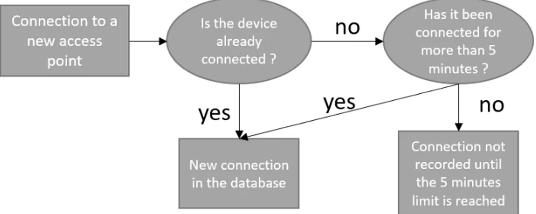
Another issue particular to our database is the aggregation of some connection time on our data : the connections with a real duration under five minutes are recorded with a five minute time duration or are not recorded. This phenomenon can be due to the data collection process or a pre-processing realized to alight the size of the data. We observe the absence of any connection with a time duration inferior to five minutes in our database. This phenomenon not representative of the actual behaviors of devices that connect for few seconds when they are transitioning between APs in a corridor, for example. The fit between the disconnection time of the connection and the connection time of the next connection prove that the connections under five minutes are not simply removed from the database. If it was the case, we would observe short time gaps between these successive connections. It appears that the connection under five minutes are aggregated with the five minutes connection as shown in Figure 3.3. The consequence of such an approximation is the loss in the accuracy of the low duration connections. In our methodology, we aggregate our data with a step of 5 minutes to have a comparable level of accuracy between our different variables.
As mentioned in the literature, one of the most common errors encountered in the Wi-Fi log data is the ping pong effect : a user located can alternatively switch between two APs when
Figure 3.3 Time aggregation process
the strength of the signal received is comparable. A consequence of it is the creation of non representative trips within the database. Different methods have been proposed to identify and limit the records of such false trips in the database, especially a spatial aggregation process within the APs. In our case, the previous aggregation of the connections under five minutes already smooth the high frequency changes of APs. The disaggregate spatial scale of our study does not allow us to spatially merge APs. In consequence, we aggregate temporally the connections showing a periodic and short switch between two points. If a device shows a series of connections of five minutes alternating between two APs, we report all sets of connections to the points representing the higher amount of time.
3.2.2 Indicators
In this document we analyze different indicators generated for the clustering and discuss their physical interpretations. The purpose of these indicators is to provide a way to characterize the user’s behaviors around each AP with interpretable variables. Some indicators generated are sensitive to the level of aggregation used. We first aggregated our connection data to five minutes to respect the constraint given by the input data as mentioned previously. Then, the indicators are computed for given duration (a day in the case of our article) creating a second aggregation bias. If the variables used to characterize the variation the number of users might seem simplistic compared to some signal treatment process, they allowed to take into consideration other variables in the clustering as the time spent by users. The limitation of the day aggregation of the indicators is answered in the discussion section of the thesis, using the decomposition of the days into smaller time intervals to improve the accuracy of the characterization of the AP use. In the following section, we use the data of the Friday 06 of