COMPLEXITÉ ET CASSAGE DE SYMÉTRIE POUR LE PROBLÈME DE LA DÉFICIENCE D’UN GRAPHE
SIVAN ALTINAKAR
DÉPARTEMENT DE MATHÉMATIQUES ET DE GÉNIE INDUSTRIEL ÉCOLE POLYTECHNIQUE DE MONTRÉAL
THÈSE PRÉSENTÉE EN VUE DE L’OBTENTION DU DIPLÔME DE PHILOSOPHIÆ DOCTOR
(MATHÉMATIQUES DE L’INGÉNIEUR) SEPTEMBRE 2016
c
ÉCOLE POLYTECHNIQUE DE MONTRÉAL
Cette thèse intitulée :
COMPLEXITÉ ET CASSAGE DE SYMÉTRIE POUR LE PROBLÈME DE LA DÉFICIENCE D’UN GRAPHE
présentée par : ALTINAKAR Sivan
en vue de l’obtention du diplôme de : Philosophiæ Doctor a été dûment acceptée par le jury d’examen constitué de :
M. SOUMIS François, Ph. D., président
M. HERTZ Alain, Doct. ès Sc., membre et directeur de recherche M. CAPOROSSI Gilles, Ph. D., membre et codirecteur de recherche Mme MARCOTTE Odile, Ph. D., membre
DÉDICACE
REMERCIEMENTS
À toutes les personnes qui ont fait partie de ma vie lors de ce voyage initiatique qu’est une thèse, je tiens à personnellement témoigner...
Ma reconnaissance sans bornes à mes deux co-directeurs Alain Hertz et Gilles Caporossi, qui n’ont jamais failli à me soutenir dans l’inconnu et les moments de contraintes, et dont la patience à mon égard mériterait d’être racontée dans une épopée.
Mes remerciements aux membres de mon jury Wieslaw Kubiak, Odile Marcotte et François Soumis, pour avoir accepté de faire partie de mon jury de thèse.
Mon affection émue à mes parents, qui m’ont encouragé dans cette voie, et qui ont généreu-sement choisi le difficile chemin de me pousser au-delà de ce que je pensais être capable, et ont accepté d’en assumer les contraignantes conséquences.
Mes belles pensées à Deborah Ummel, avec qui je me suis lancé dans cette aventure. . . et sans qui je ne l’aurais jamais terminée.
RÉSUMÉ
Une coloration d’arête d’un graphe G = (V, E) est une fonction c qui assigne un entier c(e) (appelé une couleur) dans {0, 1, 2, . . .} à chaque arête e ∈ E de sorte que des couleurs différentes soient assignées à des arêtes adjacentes. Une coloration d’arête est compacte si les couleurs des arêtes incidentes à chaque sommet forment un ensemble d’entiers consécutifs. Le problème appelé déficience consiste à déterminer le nombre minimum d’arêtes pendantes à rajouter au graphe pour que le graphe résultant ait une coloration d’arête compacte. Parmi les variations de ce problème, on compte le problème de la coloration d’arête compacte linéaire (k − LCCP ) où il est possible d’utiliser uniquement les k couleurs dans {0, 1, . . . , k − 1}, et le problème de la coloration d’arête compacte cyclique (k − CCCP ) où additionnellement la couleur 0 est considérée consécutive à la couleur k − 1.
Nous proposons une réduction polynomiale du k − LCCP (optionnellement avec des couleurs imposées ou interdites sur certaines arêtes) au k − CCCP lorsque k ≥ 12, et au 12-CCCP lorsque k < 12. Nous proposons et comparons également la performance de 3 modélisations en Programmation en Nombres Entiers et un modèle en Programmation par Contraintes pour le problème de la déficience, et déterminons le dernier comme étant le plus approprié pour ce problème.
En raison des symétries, une instance du problème de déficience peut avoir de nombreuses solutions optimales équivalentes. Nous présentons une approche pour générer un petit en-semble de contraintes, appelées GAMBLLE, destinée à casser la symétrie, qui peuvent être incorporées au modèle en programmation par contrainte. Les contraintes GAMBLLE sont inspirées des contraintes de Lex-Leader, basées sur les automorphismes de graphe, et agissent sur des familles de variables permutables. Nous analysons leur impact sur la réduction du nombre de solutions optimales, ainsi que le gain de temps obtenu lors de la résolution d’une modélisation en programmation par contrainte.
ABSTRACT
An edge-coloring of a graph G = (V, E) is a function c that assigns an integer c(e) (called color) in {0, 1, 2, . . .} to every edge e ∈ E so that adjacent edges are assigned different colors. An edge-coloring is compact if the colors of the edges incident to every vertex form a set of consecutive integers. The deficiency problem is to determine the minimum number of pendant edges that must be added to a graph such that the resulting graph admits a compact edge-coloring. Variations of this problem include the linear compact k-edge-coloring problem (k − LCCP ) where there are only the k colors of {0, 1, . . . , k − 1} available, and the cyclic compact k-edge-coloring problem (k − CCCP ) where additionally color 0 is considered consecutive to color k − 1.
We demonstrate a polynomial reduction of the k−LCCP (with optionally additional imposed or forbidden colors on some edges) to the k − CCCP when k ≥ 12, and to the 12 − CCCP when k < 12. We also propose and compare the performance of three integer programming models and one constraint programming model for the deficiency problem, and determine the latter to be the best suited to model this problem.
Because of symmetries, an instance of the deficiency problem can have many equivalent optimal solutions. We present a way to generate a small set of symmetry breaking constraints, called GAMBLLE constraints, that can be added to a constraint programming model. The GAMBLLE constraints are inspired by the Lex-Leader ones, based on automorphisms of graphs, and act on families of permutable variables. We analyze their impact on the reduction of the number of optimal solutions as well as on the speed-up of the constraint programming model.
TABLE DES MATIÈRES
DÉDICACE . . . iii
REMERCIEMENTS . . . iv
RÉSUMÉ . . . v
ABSTRACT . . . vi
TABLE DES MATIÈRES . . . vii
LISTE DES TABLEAUX . . . ix
LISTE DES FIGURES . . . x
LISTE DES SIGLES ET ABRÉVIATIONS . . . xii
CHAPITRE 1 INTRODUCTION . . . 1
1.1 Définitions et concepts de base . . . 1
1.2 Éléments de la problématique . . . 3
1.3 Objectifs de recherche . . . 5
1.4 Plan du mémoire . . . 6
CHAPITRE 2 REVUE DE LITTÉRATURE . . . 7
CHAPITRE 3 DÉMARCHE DE L’ENSEMBLE DU TRAVAIL DE RECHERCHE ET ORGANISATION DE LA THÈSE . . . 9
CHAPITRE 4 ARTICLE 1 : ON COMPACT k-EDGE-COLORINGS : A POLYNO-MIAL TIME REDUCTION FROM LINEAR TO CYCLIC . . . 11
4.1 Introduction . . . 11
4.2 Reduction of the k − LCCP to the k − CCCP . . . 16
4.3 Imposing and forbidding colors . . . 24
4.4 Non-preemptive cyclic production scheduling . . . 28
4.5 Conclusion . . . 29
4.6 Acknowledgements . . . 30 CHAPITRE 5 ARTICLE 2: A COMPARISON OF INTEGER AND CONSTRAINT
PROGRAMMING MODELS FOR THE DEFICIENCY PROBLEM . . . 31
5.1 Introduction . . . 31
5.2 An upper bound on the number of colors. . . 33
5.3 Models . . . 35
5.3.1 Integer linear programming models . . . 36
5.3.2 A constraint programming model (CP) . . . 38
5.4 Computational results . . . 40
5.4.1 Experimental setup . . . 40
5.4.2 Model comparisons for dataset D1 . . . 40
5.4.3 Model comparisons for dataset D2 . . . 42
5.4.4 Other remarks . . . 45
5.5 Conclusion . . . 46
CHAPITRE 6 ARTICLE 3: SYMMETRY BREAKING CONSTRAINTS FOR THE MINIMUM DEFICIENCY PROBLEM . . . 48
6.1 Introduction . . . 48
6.2 Model . . . 50
6.3 Graph automorphisms . . . 51
6.4 Methods for identifying automorphisms . . . 52
6.4.1 nauty . . . . 52
6.4.2 clusters . . . . 53
6.5 GAMBLLE constraints . . . 54
6.6 Computational experiments . . . 59
6.6.1 Experimental setup . . . 59
6.6.2 Automorphism group classes . . . 59
6.6.3 Comparison of algorithms . . . 62
6.7 Conclusion . . . 69
CHAPITRE 7 DISCUSSION GÉNÉRALE . . . 71
7.1 Synthèse des travaux . . . 71
7.2 Limitations des solutions proposées . . . 72
7.3 Améliorations futures . . . 73
CHAPITRE 8 CONCLUSION ET RECOMMANDATIONS . . . 74
LISTE DES TABLEAUX
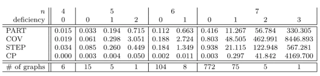
Table 5.1 Mean computing times for dataset D1, with n ≤ 7. . . . 41
Table 5.2 Pairwise comparisons for dataset D1, with n ≤ 7. . . . 41
Table 5.3 The distribution of all graphs G with 4 ≤ n ≤ 8 vertices, according to their number m of edges and their deficiency. . . . 44
Table 5.4 Values of N (f ) and N0(f ). . . . 45
Table 6.1 Automorphism group classes. . . 60
Table 6.2 gN(G) versus gC(G) for n = 8 . . . . 62
Table 6.3 d(G) versus gN(G) and the automorphism group classes. . . . 62
Table 6.4 Size of the optimal solution spaces for the proposed algorithms. . . . 64
Table 6.5 Computing times (in seconds) for six graphs. . . 67
Table 6.6 Total computing times (in seconds) to solve all the graphs with 4, 5, 6, 7 and 8 vertices . . . 68
Table 6.7 Computing times for three variants of the proposed algorithms applied to G9. . . 69
LISTE DES FIGURES
Figure 1.1 Une 3-coloration d’arêtes cyclique compacte qui n’est pas linéaire
cy-clique. . . 3
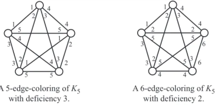
Figure 1.2 La déficience minimum du K5 ne peut être obtenue qu’en utilisant au moins ∆(G) + 2 couleurs. . . . 4
Figure 2.1 r-circulaire compact versus cyclique compact pour un non-entier r. . 8
Figure 4.1 A cyclic compact 3-edge-coloring that is not linear compact. . . 12
Figure 4.2 r-circular compact versus cyclic compact for non-integer r. . . . 13
Figure 4.3 Reduction of the LCCP to the CCCP . . . . 15
Figure 4.4 A q-bundle linking vertices u and v. . . . 16
Figure 4.5 Part of the graph Ht. . . 17
Figure 4.6 Two cyclic compact 4-edge-colorings of a graph. . . 18
Figure 4.7 An s-shift. . . . 19
Figure 4.8 An equalizer for u, v, u0, v0. . . 20
Figure 4.9 Two k-cyclic compact edge-colorings of an equalizer for u, v, u0, v0. . . 22
Figure 4.10 Illustration of T (G). . . . 22
Figure 4.11 Illustration of ˜T (G) for k = 10. . . . 24
Figure 4.12 Part of the graph PH. . . 25
Figure 4.13 Equalizers for forbidding or imposing colors. . . 27
Figure 5.1 The minimum deficiency of K5 can only be achieved by using at least ∆(G) + 2 colors. . . . 32
Figure 5.2 k-edge-colorings of C6 with k = 2, 3, 4. . . . 33
Figure 5.3 Histograms of computing times for dataset D1, with n ≤ 7. . . . 41
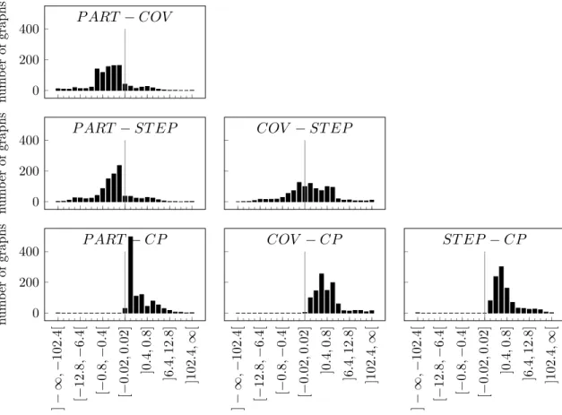
Figure 5.4 Histograms of the differences in computing times for dataset D1, with n ≤ 7. . . . 43
Figure 5.5 All graphs with n = 6 and 8 vertices and with largest deficiency. . . . 44
Figure 5.6 The none feasible, all feasible, none solved and all solved curves of the four models. . . 45
Figure 5.7 The all solved curves. . . 46
Figure 5.8 Maximum, minimum and average deficiencies of the feasible solutions found by STEP and CP in RNf0(f ). . . 46
Figure 6.1 Automorphisms and optimal edge-colorings for P4 and K3. . . 52
Figure 6.2 A graph with clique and stable sets of twins. . . 53
Figure 6.4 Illustration of the generation of gamblle constraints. . . . 57
Figure 6.5 gamblle constraints for two different edge orderings of a binary tree. 58 Figure 6.6 The smallest graph G with CAut(G) = Aut(G) = {Id}. . . . 60
Figure 6.7 Distribution of the automorphism group classes for dataset D1. . . . 61
Figure 6.8 Distribution of the automorphism group classes for dataset D2. . . . 61
Figure 6.9 Illustration of swappings on cycles and paths. . . 63
Figure 6.10 Four graphs with 5 vertices. . . 64
Figure 6.11 Optimal solutions spaces Halg(G1) for G1. . . 65
Figure 6.12 Optimal solution spaces Halg(G2) for G2. . . 65
Figure 6.13 Optimal solution spaces Halg(G3) for G3. . . 66
Figure 6.14 Optimal solution spaces Halg(G4) for G4. . . 66
Figure 6.15 Six graphs with 6 and 7 vertices. . . 67
LISTE DES SIGLES ET ABRÉVIATIONS
LCCP Linear Compact (edge-)Coloring Problem CCCP Cyclic Compact (edge-)Coloring Problem k-LCCP Linear Compact k-(edge-)Coloring Problem k-CCCP Cyclic Compact k-(edge-)Coloring Problem
CHAPITRE 1 INTRODUCTION
La déficience, définie dans le cadre de la théorie des graphes, est un invariant de graphe. Son origine provient d’un problème de confection d’horaire où certains agents doivent avoir un horaire le plus compact possible, modélisé sous la forme d’un problème de coloration d’arêtes. Il existe en particulier une variation intéressante où un horaire est amené à se répéter de manière périodique, qui peut être comparé au problème original. Par ailleurs, il n’existe pas d’algorithme exact efficace pour résoudre ce problème, même pour des petits graphes. Cette difficulté provient en partie d’un grand nombre de solutions optimales équivalentes, engendrées par les automorphismes du graphe. Pour faciliter le travail d’un solveur, il est possible, par exemple, de rajouter des contraintes destinées à briser cette symétrie.
1.1 Définitions et concepts de base
Tous les graphes considérés n’ont pas de boucle, et peuvent avoir des arêtes multiples. Une k-coloration d’arête d’un graphe G = (V, E) est une fonction c : E → {0, 1, · · · , k − 1} qui assigne une couleur c(e) à toute arête e ∈ E telle que c(e) 6= c(e0) si e et e0 partagent
une même extrêmité. Soit Ev l’ensemble des arêtes incidentes au sommet v ∈ V . Le degré
deg(v) = |Ev| de v est le nombre d’arêtes incidentes à v, et le degré maximum présent dans
G est noté ∆(G). Toute coloration d’arêtes d’un graphe G utilise au moins ∆(G) couleurs, et donc k ≥ ∆(G).
Une k-coloration d’arêtes d’un graphe G = (V, E) est (linéaire) compacte si {c(e) : e ∈ Ev}
est un ensemble d’entiers consécutifs pour tout sommet v ∈ V . Un graphe est linéaire compact colorable s’il admet une k-coloration d’arêtes linéaire compacte pour un certain entier k. Soit une k-coloration d’arêtes c de G, cmin(v) = mine∈Ev{c(e)} et cmax(v) = maxe∈Ev{c(e)} défi-nissent respectivement la plus petite et la plus grande couleur assignée à une arête incidente à v. Si c est linéaire compacte, ces dernières sont liées par cmax(v) = cmin(v) + deg(v) − 1
pour tout sommet v ∈ V . Le problème consistant à déterminer si G est k-colorable linéaire compact est noté k-LCCP (pour Linear Compact k-Coloring Problem).
Une k-coloration d’arêtes est cyclique compacte s’il existe deux entiers av, bv < k pour chaque
sommet v tel que {c(e) : e ∈ Ev} = {av, (av+ 1)mod k, · · · , (av+ |Ev| − 1)mod k = bv} (i.e.
la couleur 0 est considérée consécutive à k − 1). Un graphe est cyclique compact colorable s’il admet une k-coloration d’arêtes compacte pour un entier k. Le problème consistant à déterminer si G est k-colorable cyclique compact est noté k-CCCP (pour Cyclic Compact
k-Coloring Problem).
Par exemple, le open shop problem peut facilement se modéliser en ces termes. Il se base sur m processeurs P1, · · · , Pm et n jobs J1, · · · , Jn. Chaque job Ji est un ensemble si de
tâches. Supposons que chaque tâche doit être traitée en une unité de temps sur un processeur spécifique. Deux tâches du même job ne peuvent être traitées simultanément, et un processeur ne peut travailler sur deux tâches en même temps. Une contrainte de compacité requiert qu’aucun job n’ait de temps d’attente entre ses tâches, et qu’aucun processeur n’ait de temps d’inutilisation entre ses tâches. En d’autres mots, les périodes de temps affectées aux tâches d’un job doivent être consécutives, et chaque processeur doit être actif pendant un ensemble consécutif de périodes. L’existence d’un horaire réalisable compact sur k périodes de temps est équivalent à déterminer l’existence d’une k-coloration d’arêtes linéaire compacte du graphe G qui contient un sommet pour chaque job et chaque processeur, et une arête pour chaque tâche (i.e. une tâche d’un job Ji à traiter sur Pj est représentée par une arête entre les sommets
représentant Ji et Pj). Chaque couleur utilisée dans la k-coloration correspond à une période
de temps. La contrainte de compacité pour chaque job et processeur est équivalente à imposer que les couleurs affectées aux arêtes de Ev doivent être consécutives pour chaque sommet v
de G. Dans nombre de systèmes de production automatisée, la production est organisée d’une manière cyclique, i.e. le même horaire de production de durée T doit être répété en continu à chaque T unité de temps. La contrainte de compacité impose alors que les périodes de temps assignées aux tâches de chaque job et les périodes d’activité de chaque processeur forment des intervalles cycliques dans chaque cycle de production. L’existence d’un horaire réalisable cyclique compact est équivalent à déterminer l’existence d’une T -coloration d’arêtes cyclique compacte du même graphe G.
Soit une k-coloration d’arêtes c du graphe G et un sommet v. La déficience de c en v, notée dv(G, c), est le nombre minimum d’entiers à rajouter à {c(e) : e ∈ Ev} pour en faire une
ensemble d’entiers consécutifs. La déficience de c est définie comme la somme d(G, c) =
P
v∈V dv(G, c). D’où, c est (linéaire) compact si et seulement si d(G, c) = 0. La déficience
d’un graphe G, notée d(G), est la déficience minimale d(G, c) sur l’ensemble des colorations d’arêtes c de G. Ce concept définit une mesure qui indique à quel point G est proche d’être colorable de manière compacte. En effet, d(G) est le nombre minimum d’arêtes pendantes à rajouter à G pour que le graphe résultant soit colorable compact. Finalement, S(G) est le plus grand entier tel que G admette une S(G)-coloration d’arêtes c de déficience d(G, c) = d(G) et utilisant toutes les S(G) couleurs.
Dans l’exemple précédent de open shop dans le cas linéaire, si les temps d’attente des jobs et des processeurs ne sont pas interdits, leur nombre devant cependant être minimisé, alors le
problème devient équivalent à trouver une coloration d’arêtes de G avec déficience minimum. Pour terminer, un automorphisme d’un graphe G = (V, E) est une permutation σ de l’en-semble de ses sommets V tel que (u, v) ∈ E ⇔ (σ(u), σ(v)) ∈ E. Ce nouvel ordre des sommets de G préserve donc la matrice d’adjacence.
1.2 Éléments de la problématique
Le problème de déterminer si un graphe admet une k-coloration d’arêtes linéaire compacte (k-LCCP) est fréquent dans les problèmes de confection d’horaire avec contraintes de com-pacité (Giaro et al., 1999a). Il est N P-complet (Sevastianov, 1990), même pour les graphes bipartis.
Si k0 > k et que G admet une k-coloration d’arêtes linéaire compacte, alors il admet aussi un k0-coloration d’arêtes linéaire compacte. Par contre, cette propriété n’est pas vraie en général pour le cas cyclique compact, comme avec le triangle et le pentagone qui admettent une 3-coloration d’arêtes cyclique compacte, mais pas une 4-3-coloration d’arêtes cyclique compacte. De plus, une k-coloration d’arêtes linéaire compacte est également cyclique compacte (avec av = cmin(v) et bv = cmax(v)), mais l’inverse n’est pas nécessairement vrai. Par exemple, la
3-coloration d’arêtes du triangle de la Figure 1.1 est cyclique compacte, mais pas linéaire compacte (car la couleur 1 est absente dans {c(e)|e ∈ Eb}). Il n’est pas difficile de remarquer
que le triangle n’est pas linéaire compact colorable.
a b
c 0
1 2
Figure 1.1 Une 3-coloration d’arêtes cyclique compacte qui n’est pas linéaire cyclique.
Le problème de déterminer si un graphe admet une coloration d’arêtes cyclique compacte (CCCP) a été démontré N P-complet (Kubale and Nadolski, 2005), à l’aide d’une réduction en temps polynomial de tout problème de LCCP en un CCCP. Cette réduction ne préserve pas le nombre k de couleurs utilisées. Par contre, elle préserve la bipartition, ce qui démontre que le CCCP est N P-complet même pour le cas biparti.
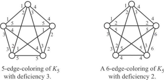
Le théorème de Vizing (Vizing, 1964) garantit l’existence d’une k-coloration d’arêtes pour tout k ≥ ∆(G) + 1 couleurs. Par exemple, il n’est pas difficile de vérifier que la clique K5
que toute 5-coloration d’arêtes c de K5 a une déficience de d(K5, c) = 3. Cependant, comme
illustré sur la Figure 1.2, il est facile de colorier les arêtes de K5 avec six couleurs et une
déficience de 2. 1 2 3 4 5 4 3 5 2 1 A 6-edge-coloring of K5 with deficiency 2. A 5-edge-coloring of K5 with deficiency 3. 1 5 4 5 2 3 4 21 3 1 2 3 4 2 5 3 4 6 5 1 2 4 4 6 3 5 25 3
Figure 1.2 La déficience minimum du K5 ne peut être obtenue qu’en utilisant au moins
∆(G) + 2 couleurs.
Il n’existe pas encore d’algorithme exact efficace pour déterminer la déficience d’un graphe. Le premier défi rencontré pour résoudre ce problème est l’absence de borne supérieure K raisonnable sur le nombre minimum de couleurs à utiliser pour pouvoir colorier le graphe de manière optimale. Certaines modélisations requièrent une telle borne K, lorsqu’une famille de variables identiques est définie pour chaque couleur permise. Un exemple est une modé-lisation en Programmation en Nombres Entiers, avec une variable binaire ce,k ∈ {0, 1} pour
représenter la coloration d’une arête v ∈ E par la couleur 0 ≤ k ≤ K, dans une contrainte du genreP
0≤k≤Kce,k = 1. Un nombre K trop petit donnera une k-coloration déficiente optimale
pour ce nombre de couleur K, mais non-optimale en général, comme vu précédemment pour le K5. Et, dans le cas opposé, un trop grand nombre de couleurs va impliquer la génération
d’un nombre important de variables inutiles et leurs contraintes associées, ce qui va naturel-lement se répercuter sur la performance d’un solveur utilisé pour résoudre l’instance, incluant son utilisation de mémoire. Il est bien sûr possible de modéliser ce problème sans avoir besoin d’une telle borne, ce qui entraîne d’autres avantages et difficultés. Une borne supérieure sur S(G) serait par exemple une option pour K, mais la seule existante n’est valide que pour les cas sans déficience.
Un deuxième défi important, dans le contexte de la déficience, est le nombre très important de solutions optimales équivalentes (i.e. de même déficience optimale) qu’il existe pour un graphe donné G. La structure du problème en permet souvent plusieurs, et celles-ci peuvent être regroupées en classes d’équivalence lorsque l’une peut être obtenue à partir d’une autre par symétrie, sous l’effet d’un automorphisme du graphe. Par exemple, soit le chemin de longueur 4 noté P4, constitué de trois arêtes successives e1, e2et e3, avec l’une de ses solutions exprimées
par le triplet (c(e1), c(e2), c(e3)). Il existe un automorphisme pour ce graphe, qui échange e1
et e3, et laisse e2 fixe. Ce graphe a quatre solutions optimales : s1 = (0, 1, 0), s2 = (1, 0, 1),
s3 = (0, 1, 2) et s4 = (2, 1, 0). Elles se partitionnent en trois classes d’équivalence {s1}, {s2}
et {s3, s4}, et le dernier contient deux solutions symétriques.
Dans le cas d’un graphe de petite taille, le solveur arrive souvent à atteindre la solution optimale très rapidement, c’est alors la preuve d’optimalité qui s’avère être problématique. Ces solutions équivalentes donnent souvent l’illusion à l’algorithme d’énumération implicite qu’une branche pourrait donner une meilleure solution que l’optimale, avant d’avoir été étu-diée en profondeur, après quoi il se révèle qu’elles ne font que redonner une autre solution optimale.
1.3 Objectifs de recherche
Dans le but de démontrer plus explicitement le lien entre le k-LCCP et le k-CCCP pour un k fixé, nous proposons dans cette thèse une réduction en temps polynomial d’un k-LCCP en un k-CCCP pour tout graphe G et pour tout entier k ≥ 12. Pour des valeurs plus petites de k, nous montrons qu’un k-LCCP peut être réduit en un 12-CCCP. Notre outil fondamental pour cette réduction est une transformation de graphe qui permet de garantir que deux arêtes non-adjacentes vont être affectées de la même couleur. Comme corollaire, cette transformation nous permet d’imposer ou d’interdire une couleur donnée sur n’importe quelle arête du graphe. Ceci s’avère utile en particulier dans des problèmes d’ordonnancement où certaines tâches doivent être exécutées à des périodes de temps spécifiques. De plus, nous démontrons que déterminer un horaire de production cyclique sans préemption de longueur k (avec possiblement des temps de traitement non-uniformes) est équivalent à résoudre un k-CCCP dans un graphe approprié.
Pour la déficience, nous proposons une borne supérieure pour S(G) valable pour tout graphe, et nous l’utilisons ensuite pour proposer trois modélisations en Programmation en Nombres Entiers pour résoudre ce problème de manière exacte. Nous comparons la performance de ces modélisations entre elles et à une modélisation en Programmation par Contrainte, et déterminons ce dernier comme étant le plus performant et approprié des quatre pour mo-déliser ce problème. Nous nous concentrons ensuite en particulier sur ce dernier modèle afin de l’améliorer en définissant des méthodes pour y rajouter des contraintes dépendantes du graphe étudié, appelées contraintes GAMBLLE, qui vont permettre de briser une partie de la symétrie présente. Nous analysons leur impact sur la réduction du nombre de solutions optimales et sur le temps de résolution.
1.4 Plan du mémoire
Le présent document est structuré comme suit. Le chapitre 2 regroupe une revue de littéra-ture sur le problème de la déficience et ses variantes, ainsi que des techniques de cassage de symétrie. Le chapitre 3 présente la démarche de l’ensemble du travail de recherche et l’orga-nisation de la thèse. Le chapitre 4 est un article publié dans Discrete Optimization, étudiant la complexité de déterminer la déficience d’un graphe dans un cas de couleurs cycliques. Le chapitre 5 est un article publié dans Computers & Operations Research, comparant des mo-délisations du problème de la déficience, trois en programmation par nombres entiers et un en programmation par contrainte. Le chapitre 6 est un article soumis à Computers & Ope-rations Research, et perfectionne ce dernier modèle en y ajoutant des contraintes pour briser une partie de la symétrie engendrée par les automorphismes du graphe. Pour terminer, le chapitre 7 présente une discussion plus générale, portant sur l’ensemble du travail accompli, et le chapitre 8 conclut ce document.
CHAPITRE 2 REVUE DE LITTÉRATURE
Le terme coloration d’arêtes (linéaire) compacte est équivalent aux termes coloration d’arêtes consécutive (Giaro, 1997; Giaro et al., 2001) et coloration d’arêtes par intervalle (Asratian and Casselgren, 2006; Asratian and Kamalian, 1987; Hanson and Loten, 1996; Hanson et al., 1998; Pyatkin, 2004; Sevastianov, 1990), utilisé par certains auteurs. Le problème de déterminer si un graphe admet une k-coloration d’arêtes linéaire compacte (k-LCCP) a été proposé par Asratian and Kamalian (1987). C’est une problématique fréquente dans les problèmes de confection d’horaire avec contraintes de compacité (Giaro et al., 1999a). Il est N P-complet (Sevastianov, 1990), même pour les graphes bipartis.
Le problème de déterminer si un graphe admet une k-coloration d’arêtes cyclique compacte (k-CCCP) est étudié dans Nadolski (2008), ainsi que dans Kubale and Nadolski (2005). Dans ce dernier, il est démontré que le CCCP est N P-complet, même pour le cas biparti.
La k-coloration d’arêtes cyclique compacte est à rapprocher de la coloration d’arêtes circulaire compacte définie dans Kubale and Nadolski (2005). Soit un nombre réel positif r, Cr définit
le cercle de circonférence r. Soit un point 0 ∈ Cr arbitraire et une orientation, tous les deux arbitraires, (a, b) représente l’arc ouvert commençant en a et se terminant en b, où a, b ∈ [0, r]. La longueur d’un arc (a, b) est b − a si b > a et r − a + b si b < a. Une coloration d’arêtes r-circulaire est une affectation d’un arc ouvert A(e) ⊂ Crde longueur 1 à chaque arête e tel que
A(e) et A(e0) sont disjoints quand e et e0 ont une extrêmité en commun. Une telle coloration est compacte si la fermeture de l’union des arcs ouverts affectées aux arêtes de Ev est un arc
sur Crpour tout sommet v. Quand r est un entier, la coloration d’arêtes r-circulaire compacte
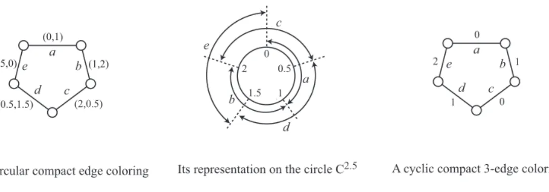
est équivalente à la coloration d’arêtes cyclique compacte. Pour les valeurs non-entières de r, la situation est légèrement différente. Par exemple, comme présenté à la Figure 2.1, il existe une coloration d’arêtes r-circulaire compacte du pentagone avec r = 2.5, alors qu’il est facile d’observer que toute k-coloration d’arêtes cyclique compacte du pentagone nécessite k ≥ 3, avec un exemple d’une 3-coloration d’arêtes cyclique compacte présentée à droite dans la Figure 2.1.
Le concept de déficience a été proposé par Giaro et al. (1999b), et déterminer la déficience d’un graphe est N P-difficile (Giaro, 1997). Ce problème est aussi étudié dans Asratian and Casselgren (2006); Bouchard et al. (2009); Giaro et al. (2001); Hanson and Loten (1996); Hanson et al. (1998); Pyatkin (2004); Schwartz (2006). À notre connaisance, il n’existe pas encore d’algorithme exact efficace pour déterminer la déficience d’un graphe. Le principal travail dans une direction similaire est une heuristique par Bouchard et al. (2009) basée sur
a b c (0,1) (1,2) d e (2,0.5) (0.5,1.5) (1.5,0) 0 0.5 1.5 1 2 a b c d e a b c 0 1 d e 0 1 2
A 2.5-circular compact edge coloring Its representation on the circle C2.5 A cyclic compact 3-edge coloring
Figure 2.1 r-circulaire compact versus cyclique compact pour un non-entier r.
une recherche tabou. Aussi, Giaro et al. (2001) ont prouvé que dans le cas d’un graphe G colorable compactement (i.e. d(G) = 0) que S(G) ≤ 2n − 4, où n est le nombre de sommets de G.
Plusieurs auteurs ont chacun identifié et classifié de manières différentes les nombreux types de symétrie dans leur contexte de recherche respectif. Cette thèse adopte la terminologie de Cohen et al. (2006); Gent et al. (2006), qui classifie en deux catégories générales les symétries de solution et de problème (ou contrainte). De telles permutations de l’ensemble de paires (variable,valeur ) préservent respectivement la solution ou les contraintes du problème. De plus, la dernière est un sous-ensemble de la première. Il est intéressant de relever qu’identifier les symétries du premier type requiert habituellement de trouver d’abord toutes les solutions, alors que celles du deuxième type peuvent être déduites de la structure et de l’expression du problème. Et, par ailleurs, ces deux types ont chacun deux cas spéciaux de symétrie de variable et valeurs, qui permutent respectivement seulement les variables ou les valeurs. La Méthode de Lex-Leader proposée par Crawford et al. (1996), et par la suite améliorée dans Cohen et al. (2006); Luks and Roy (2004); Pujet (2005), est à la base de la recherche présentée dans ce travail. Elle rajoute des contraintes de façon à ne garder qu’un représentant de chaque classe d’équivalence. Une telle méthode peut requérir que l’on rajoute un énorme nombre de contraintes au modèle, et parfois les rajouter peut s’avérer contre-productif.
CHAPITRE 3 DÉMARCHE DE L’ENSEMBLE DU TRAVAIL DE RECHERCHE ET ORGANISATION DE LA THÈSE
Cette thèse a pour objectif d’étudier et d’améliorer la compréhension d’une famille de pro-blèmes basés sur le concept d’une coloration d’arêtes que l’on essaie de rendre le plus compacte possible. Cette famille demeure peu étudiée, et le chapitre 2 synthétise les travaux précédant le nôtre.
Un des membres de cette famille est la k-coloration d’arête cyclique compacte. Il existait déjà une preuve que ce problème est N P-complet, utilisant une réduction polynomiale à partir du problème de la k-coloration d’arête (linéaire) compacte. Cependant, cette réduction ne conserve pas le nombre de couleurs k. Nous avons donc proposé dans le chapitre 4 une nouvelle réduction polynomiale ayant cette propriété supplémentaire. Notre réduction est fondée sur l’utilisation judicieuse d’un sous-graphe appelé equalizer, ayant la propriété de simuler deux arêtes étant forcées à avoir la même couleur dans n’importe quelle coloration d’arête valide du graphe. La portée d’un tel outil dépasse bien largement le cadre de notre réduction, et nous montrons également comment le mettre à profit pour exprimer à l’aide d’une k-coloration d’arête cyclique compacte toutes sortes de variantes dans cette famille de problèmes étudiés. Un autre volet dans cette famille de problèmes est celui de déterminer la déficience minimale d’une coloration d’arêtes. Nous avons choisi dans le chapitre 5 de tester plusieurs modèles en Programmation en Nombres Entiers et un en Programmation par Contraintes. Ces modèles sont tous destinés à déterminer la déficience de manière exacte, en s’appuyant sur un solveur. Pour rendre possible ces modélisations, nous avons dû déterminer une borne supérieure sur le nombre de couleurs à utiliser. Au terme d’une série de comparaisons de leur performance sur des graphes jusqu’à 100 sommets, il a été déterminé que le modèle en Programmation par Contraintes est clairement le plus performant.
Ces tests ont également mis en lumière une des difficultés majeures pour résoudre ce pro-blème. Dans les graphes de petite taille de neuf sommets ou moins, atteindre une solution optimale est extrêmement aisé. Cependant, prouver l’optimalité de cette solution est ralenti souvent par une myriade de solutions optimales équivalentes. Passer à travers cet ensemble de solutions peu intéressantes concentre l’essentiel du temps de calcul. Une grande majorité de ces solutions équivalentes résultent des automorphismes du graphe examiné. Pour affiner notre procédure précédente, nous avons développé dans le chapitre 6 une méthode pour gé-nérer des contraintes aptes à briser une partie de la symétrie dans le modèle. Ces contraintes sont appelées Graph AutoMorphism Based Lex-Leader Enforcing (GAMBLLE), et sont à
ajouter à la formulation en Programmation par Contraintes avant que celle-ci ne soit résolue par un solveur. Ces contraintes s’inspirent de la méthode de Lex-Leader et s’appuient sur une liste complète ou partielle de générateurs pour le groupe d’automorphismes du graphe. Cette démarche donne lieu à un nombre extrêmement réduit de contraintes, obtenues à très peu de frais. Nos tests sur des graphes jusqu’à neuf sommets ont démontré que ce petit nombre améliore le temps de résolution de quelques ordres de magnitude. Cela est dû à la réduc-tion impressionnante de l’espace de soluréduc-tions, où bon nombre de soluréduc-tions équivalentes sont éliminées tout en conservant un représentant au minimum de chaque classe d’équivalence. Pour terminer, le chapitre 7 présente une discussion plus générale, portant sur l’ensemble du travail accompli, et le chapitre 8 conclut ce document.
CHAPITRE 4 ARTICLE 1: ON COMPACT k-EDGE-COLORINGS: A POLYNOMIAL TIME REDUCTION FROM LINEAR TO CYCLIC
Abstract
A k-edge-coloring of a graph G = (V, E) is a function c that assigns an integer c(e) (called color) in {0, 1, · · · , k − 1} to every edge e ∈ E so that adjacent edges get different colors. A k-edge-coloring is linear compact if the colors on the edges incident to every vertex are consecutive. The problem k − LCCP is to determine whether a given graph admits a linear compact k-edge coloring. A k-edge-coloring is cyclic compact if for every vertex v there are two positive integers av, bv in {0, 1, · · · , k − 1} such that the colors on the edges incident to
v are exactly {av, (av+ 1)mod k, · · · , bv}. The problem k − CCCP is to determine whether
a given graph admits a cyclic compact k-edge coloring. We show that the k − LCCP with possibly imposed or forbidden colors on some edges is polynomially reducible to the k−CCCP when k ≥ 12, and to the 12 − CCCP when k < 12.
4.1 Introduction
All graphs considered in this paper have no loops but may contain parallel edges. A k-edge-coloring of a graph G = (V, E) is a function c : E → {0, 1, · · · , k − 1} that assigns a color c(e) to every edge e ∈ E such that c(e) 6= c(e0) whenever e and e0 share a common endpoint. Let Ev denote the set of edges incident with vertex v ∈ V . The degree of a vertex v is the number
of edges in Ev and the maximum degree in G is denoted ∆(G). Note that all k-edge-colorings
of a graph G use at least ∆(G) different colors, which means that ∆(G) ≤ k.
A k-edge-coloring of a graph G = (V, E) is linear compact if {c(e) : e ∈ Ev} is a set of
consecutive integers for each vertex v ∈ V . The terms consecutive edge-colorings (Giaro, 1997; Giaro et al., 2001) and interval edge-colorings (Asratian and Casselgren, 2006; Asratian and Kamalian, 1987; Hanson and Loten, 1996; Hanson et al., 1998; Pyatkin, 2004; Sevastianov, 1990) are also used by some authors. A graph is linearly compactly colorable if it admits a linear compact k-edge-coloring for some integer k. For a k-edge-coloring c of a graph G = (V, E), let cmin(v) = mine∈Ev{c(e)} and cmax(v) = maxe∈Ev{c(e)} denote, respectively, the smallest and the largest color assigned to an edge incident to v. It follows from the above definition that if c is linear compact, then cmax(v) = cmin(v) + |Ev| − 1 for all vertices v ∈ V .
A k-edge-coloring is cyclic compact if we can associate two positive integers av, bv < k to
(i.e., color 0 is considered as consecutive to k − 1). A graph is cyclically compactly colorable if it admits a cyclic compact edge-coloring for some integer k. While linear compact k-edge-colorings are also cyclic compact (with av = cmin(v) and bv = cmax(v)), the reverse is
not necessarily true. For example, the 3-edge-coloring of the triangle shown in Figure 4.1 is cyclic compact but not linear compact (since color 1 is missing in {c(e)|e ∈ Eb}). It is not
difficult to observe that the triangle is not linearly compactly colorable.
a b
c 0
1 2
Figure 4.1 A cyclic compact 3-edge-coloring that is not linear compact.
Cyclic compact k-edge-colorings are also studied in (Nadolski, 2008) and are closely related to the circular compact colorability defined in (Kubale and Nadolski, 2005). Given a positive real number r, let Cr denote the circle with circumference r. Taking an arbitrary point 0 ∈ Cr and orientation, we denote (a, b) the open arc starting in a and ending in b, where a, b ∈ [0, r]. The length of an arc (a, b) is b − a if b > a and r − a + b if b < a. An r-circular edge-coloring is an assignment of an open arc A(e) ⊂ Cr of length 1 to each edge e so that
A(e) and A(e0) are disjoint whenever e and e0 share a common endpoint. Such a coloring is compact if the closure of the union of open arcs assigned to the edges of Ev is an arc on
Cr for each vertex v. When r is integer, compact r-circular edge-colorings are equivalent to
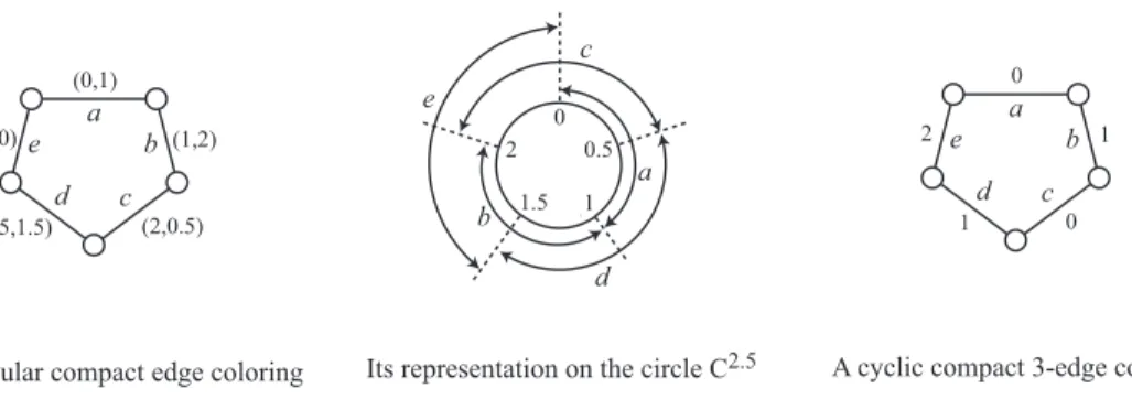
cyclic compact r-edge-colorings. For non-integer values of r, the situation is slightly different. For example, as shown in Figure 4.2, there exists a compact r-circular edge-coloring of the pentagon with r = 2.5, while it is easy to observe that all cyclic compact k-edge-colorings of the pentagon have k ≥ 3, an example of a cyclic compact 3-edge-coloring being shown on the right of Figure 4.2.
The problem of determining a linear compact k-edge-coloring (if any) of a graph was in-troduced by Asratian and Kamalian (1987). It often arises in scheduling problems with compactness constraints (Giaro et al., 1999a). For example, the open shop problem consid-ers m processors P1, · · · , Pm and n jobs J1, · · · , Jn. Each job Ji is a set of si tasks. Suppose
that each task has to be processed in one time unit on a specific processor. No two tasks of the same job can be processed simultaneously and no processor can work on two tasks at the same time. Moreover, compactness requirements state that waiting periods are forbidden for every job and no idles are allowed on each processor. In other words, the time periods assigned to the tasks of a job must be consecutive, and each processor must be active during
a b c (0,1) (1,2) d e (2,0.5) (0.5,1.5) (1.5,0) 0 0.5 1.5 1 2 a b c d e a b c 0 1 d e 0 1 2
A 2.5-circular compact edge coloring Its representation on the circle C2.5 A cyclic compact 3-edge coloring
Figure 4.2 r-circular compact versus cyclic compact for non-integer r.
a set of consecutive periods. The existence of a feasible compact schedule with k time pe-riods is equivalent to the existence of a linear compact k-edge-coloring of the graph G that contains one vertex for each job and each processor, and one edge for each task (i.e., a task of job Ji to be processed on Pj is represented by an edge between the vertices representing
Ji and Pj). Each color used in the k-edge-coloring corresponds to a time period. The
com-pactness requirements for each job and each processor are equivalent to imposing that the colors appearing on the edges of Ev must be consecutive for every vertex v in G. In many
automated production systems, the production is organized in a cyclic way, i.e., the same production schedule of length T is repeated continuously every T time units. Compactness requirements then impose that the time periods assigned to the tasks of each job and the active period of each processor form a cyclic interval in each production cycle. The existence of a feasible cyclic compact schedule is then equivalent to the existence of a cyclic compact T -edge-coloring of the same graph G.
The problem of determining whether or not a given graph is linearly compactly colorable is denoted LCCP and is known to be N P-complete (Sevastianov, 1990), even for bipartite graphs. Given a k-edge-coloring c of a graph G, let Dv(G, c) denote the minimum number of
integers which must be added to {c(e) : e ∈ Ev} to form an interval of consecutive integers.
The deficiency of c is defined as the sum D(G, c) =P
v∈V Dv(G, c). Hence, c is linear compact
if and only if D(G, c) = 0. The deficiency of a graph G, denoted Def (G), is the minimum deficiency D(G, c) over all k-edge-colorings c of G (where k can take any positive integer value). This concept, which was introduced by Giaro et al. (1999b), provides a measure of how close G is to be linearly compactly colorable since the deficiency of G is the minimum number of pendant edges that must be added to G such that the resulting graph is linearly compactly colorable. The problem of determining the deficiency of a graph is N P-hard (Giaro, 1997). This problem is also studied in (Asratian and Casselgren, 2006; Giaro et al., 1999b; Hanson and Loten, 1996; Hanson et al., 1998; Pyatkin, 2004; Schwartz, 2006; Giaro
et al., 2001; Bouchard et al., 2009).
The problem of determining whether or not a given graph is cyclically compactly colorable is denoted CCCP . To demonstrate that it is N P-complete, Kubale and Nadolski (2005) build a graph H from a graph G so that G is linearly compactly colorable if and only if H is cyclically compactly colorable. The graph H is defined as G ∪ K1,m+1, where m is the
number of edges in G and K1,m+1 is the star with m + 1 branches (i.e., the graph containing
1 vertex with degree m + 1 and m + 1 vertices with degree 1). In other words, H is obtained from G by adding a new connected component isomorphic to K1,m+1. Assume that G is
linearly compactly colorable and let k be the smallest integer such that G admits a linear compact k-edge-coloring c. We then have k ≤ m since every color in {0, · · · , k − 1} appears in c, which means that c can be extended to a cyclic compact (m + 1)-edge-coloring of H by assigning colors 0, 1, · · · , m to the edges of K1,m+1. Also, if H admits a cyclic compact
k-edge-coloring c, then k ≥ ∆(H) = m + 1. Since G contains m edges, at least one of the k colors does not appear in G and, without loss of generality, we may assume that the missing color is k − 1 (otherwise, a cyclic permutation of the colors in c leads to such a coloring), which means that no vertex v in G has both colors 0 and k − 1 in Ev. The edge-coloring c
restricted to G is therefore linear compact. In summary, G is linearly compactly colorable if and only if H is cyclically compactly colorable, and since H can be obtained from G in polynomial time (by adding m + 2 vertices and m + 1 edges), this proves that the LCCP is polynomially reducible to the CCCP , which demonstrates the N P-completeness of the CCCP . Note that H is bipartite if and only if G is bipartite, which proves that the CCCP is N P-complete even for bipartite graphs.
In this paper, we are interested in determining whether or not a given graph admits a linear (cyclic) compact k-edge-coloring for a fixed integer k.
Definition 1. Let G be a graph and k > 0 an integer.
— G is k-linearly compactly colorable if it admits a linear compact k-edge-coloring. We denote k-LCCP the problem of determining whether or not G is k-linearly compactly colorable.
— G is k-cyclically compactly colorable if it admits a cyclic compact k-edge-coloring. We denote k-CCCP the problem of determining whether or not G is k-cyclically compactly colorable.
Note that if k0 > k and G is k-linearly compactly colorable, then G is also k0-linearly com-pactly colorable. However, a k-cyclically comcom-pactly colorable graph is not necessarily k0 -cyclically compactly colorable for k0 > k. For example, the triangle and the pentagon are
3-cyclically compactly colorable while they are not 4-cyclically compactly colorable. The re-duction proposed in (Kubale and Nadolski, 2005) shows that a given graph G with m edges is m-linearly compactly colorable if and only if H is (m + 1)-cyclically compactly colorable. We note however that the linear compact m-edge-coloring of G derived from the cyclic compact (m + 1)-edge-coloring of H uses possibly up to m different colors while less colors may be sufficient. For example, consider the graph G containing a chain on 4 vertices a, b, c, d, with edges between a and b, b and c, and c and d. As shown in Figure 4.3, H is 4-cyclically com-pactly colorable, and we therefore know that G is 3-linearly comcom-pactly colorable. However, the reduction does not provide any information about the 2-linear compact colorability of G which is demonstrated by the linear compact 2-edge-coloring on the right of Figure 4.3.
0 A graph G 1 2 3 0 1 2 0 1 0
A cyclic compact 4-edge-coloring of H=G K
1,4
with a linear compact 3-edge-coloring of G
A linear compact 2-edge-coloring of G U a b d c a b d c a b d c
Figure 4.3 Reduction of the LCCP to the CCCP .
In this paper, we prove that there is a polynomial time reduction of the k − LCCP to the k − CCCP for every graph G and every integer k ≥ 12. For smaller values of k, we show that the k − LCCP can be reduced to the 12 − CCCP . These reductions are described in detail in Section 2. A basic tool in our reductions is a graph transformation which makes it possible to impose the same color on two non-adjacent edges. As a corollary, as shown in Section 3, we can impose or forbid a given color on any edge of the graph. This may be helpful when solving production scheduling problems in which some tasks can only be processed at specific time periods. We also show in Section 4 that finding a non-preemptive cyclic production schedule of length k (with possibly non-uniform processing times) is equivalent to solving a k − CCCP in an appropriate graph.
In summary, while the existence of a reduction of the k − LCCP to the k − CCCP is not surprising (since both problems are N P-complete), the proposed reduction, unlike previous transformations, does not increase the number k of colors, and makes it possible to transform a linear coloring problem with forbidden and imposed colors into a cyclic coloring problem without additional constraints.
4.2 Reduction of the k − LCCP to the k − CCCP
Note that we always assume k ≥ ∆(G) else G is obviously not k-linearly or k-cyclically compactly colorable. Also, we assume k ≤ |E| since it is easy to transform any k-linear or k-cyclic compact coloring of G with k > |E| into a |E|-linear or |E|-cyclic compact coloring of G. For k ≥ 12, we describe in this section a construction of a graph H from a graph G so that G is k-linearly compactly colorable if and only if H is k-cyclically compactly colorable. For k < 12, we slightly modify our construction of H so that G is k-linearly compactly colorable if and only if H is 12-cyclically compactly colorable.
Given two positive integers x, y < k, we denote [x, y]k the set {x mod k,
(x + 1) mod k, · · · , y mod k}. Hence, a k-edge-coloring c of a graph G is cyclic compact if we can associate two integers 0 ≤ av, bv < k to every vertex v so that {c(e) : e ∈ Ev} = [av, bv]k.
q
u v
Figure 4.4 A q-bundle linking vertices u and v.
For an integer q ≥ 1, we call q-bundle a set of q parallel edges linking two vertices u and v. When drawing a graph, q-bundles are represented as in Figure 4.4. Given a graph G, we build a new graph, denoted GB by adding a new vertex v0 for each vertex v of degree strictly
smaller than k in G and by linking each pair v, v0 of vertices with a (k − |Ev|)-bundle. We
denote EuB the set of edges incident to a vertex u in GB. The next lemma shows how to link the k − LCCP in G to the k − CCCP in GB.
Lemma 1. G is k-linearly compactly colorable if and only if GB admits a cyclic compact k-edge-coloring such that for every vertex v of G with |Ev| < k, the (k − |Ev|)-bundle added
to G contains color 0 and/or k − 1.
Proof. (⇒) Let c be a linear compact k-edge-coloring of G and let [av, bv]k denote the set of
colors on the edges of Ev incident to v in G. For vertices v with |Ev| < k, let us assign all
colors in [bv+1, av−1]k to the edges of the (k −|Ev|)-bundle linking v to v0. The edge-coloring
c is thus extended to an edge-coloring cB of GB where {cB(e) : e ∈ EB
v } = [0, k − 1]k for
every v in G, and {cB(e) : e ∈ EB
v0} = [bv + 1, av − 1]k for every new vertex v0. Hence, cB is
a cyclic compact k-edge-coloring of GB. Since c is linear compact, |[av, bv]k∩ {0, k − 1}| ≤ 1
for every vertex v with |Ev| < k. Hence, |[bv+ 1, av− 1]k∩ {0, k − 1}| ≥ 1 for these vertices,
(⇐) Let cB be a cyclic compact k-edge-coloring of GB such that every
(k − |Ev|)-bundle added to G contains color 0 and/or k − 1. For every vertex u in GB,
let [au, bu]k = {cB(e) : e ∈ EuB}. If u is a vertex in G with |Eu| = k, then {cB(e) : e ∈ Eu} =
[0, k −1]k. If u is a vertex in G with |Eu| < k then EuBcontains all edges of Euas well as those
of the (k − |Eu|)-bundle linking u to u0. Since |EuB| = k and {cB(e) : e ∈ EuB0} = [au0, bu0]k,
we have {cB(e) : e ∈ E
u} = [bu0 + 1, au0 − 1]k. Moreover, |[au0, bu0]k∩ {0, k − 1}| ≥ 1 implies
|[bu0+ 1, au0− 1]k∩ {0, k − 1}| ≤ 1, which means that the edge-coloring cB restricted to G is
a linear compact k-edge-coloring of G.
We now have to show how color 0 and/or k − 1 can be imposed on every (k − |Ev|)-bundle
added to G. Let t denote the number of vertices v in G with |Ev| < k and let Ht denote the
graph with 2t vertices u1, · · · , ut, w1, · · · , wt and such that every ui is linked to wi (1 ≤ i ≤ t)
with two parallel edges (i.e., a 2-bundle) and every wi is linked to ui+1 (1 ≤ i < t) with a
(k − 2)-bundle (see Figure 4.5). Also, let GB+ = GB∪ Ht. In other words, GB+ is obtained
from GB by adding a new connected component isomorphic to Ht. Let us label v1, · · · , vt
the vertices of G with |Evi| < k, let e
B
i be one of the edges of the (k − |Evi|)-bundle linking vi to vi0, and let eHi be one of the two edges linking ui to wi. The next lemma provides a link
between cyclic compact k-edge-colorings of GB and GB+.
ui wi k-2 ui+1 wi+1
ui-1 wi-1
k-2
Figure 4.5 Part of the graph Ht.
Lemma 2. GB admits a cyclic compact k-edge-coloring such that every (k − |E
vi|)-bundle added to G contains color 0 and/or k − 1 if and only if GB+ admits a cyclic compact
k-edge-coloring c with c(eB
i ) = c(eHi ) for i = 1, · · · , t.
Proof. (⇒) Let c be a cyclic compact k-edge-coloring of GB such that every (k −|E
vi|)-bundle added to G contains color 0 and/or k − 1. The colors on every (k − |Evi|)-bundle can be permuted to obtain a new cyclic compact k-edge coloring c0 so that eB
i gets color 0 or k − 1.
Now, assign color c0(eBi ) to eHi , color k − 1 − c0(eBi ) (i.e., the other color in {0, k − 1}) to the second edge linking ui to wi, and colors 1, · · · , k − 2 to the (k − 2)-bundle linking wi to ui+1
(if i < t). By construction, the extension of c0 to GB+ is a cyclic compact k-edge-coloring
with c0(eB i ) = c
0(eH
(⇐) Assume now that c is a cyclic compact k-edge-coloring of GB+ with c(eB
i ) = c(eHi )
for i = 1, · · · , t. Since u1 has degree 2, we can permute the colors in c in a cyclic way to
obtain a new cyclic compact k-edge coloring c0 so that the two edges incident to u1 get colors
0 and k − 1. The (k − 2)-bundle linking w1 to u2 then necessarily contains all colors in
{1, · · · , k − 2}, which means that the 2 edges linking u2 to w2 also have color 0 and k − 1.
By repeating the same reasoning, we conclude that the two edges linking ui to wi (1 ≤ i ≤ t)
have color 0 and k − 1 and the edges of the (k − 2)-bundle linking wi to ui+1 (1 ≤ i < t) have
colors 1, · · · , k − 2. Hence, c0(eH i ) = 0 or k − 1 for i = 1, · · · , t. Since c 0(eB i ) = c 0(eH i ), we
conclude that the restriction of c0 to GB is a cyclic compact k-edge-coloring such that each
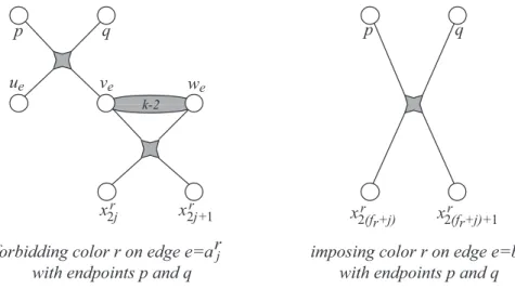
(k − |Evi|)-bundle added to G contains color 0 and/or k − 1. It remains to show how to impose the same color on eB
i and eHi (1 ≤ i ≤ t). More generally,
given two non-adjacent edges e and e0 in a graph G, we are interested in building a new graph G0 so that G0 is k-cyclically compactly colorable if and only if G admits a cyclic compact k-edge-coloring c with c(e) = c(e0). For illustration, Figure 4.6 contains two cyclic compact 4-edge-colorings of the same graph. In the left graph, the two edges e and e0 have different colors while c(e) = c(e0) = 2 in the right graph. We are interested in imposing the same color on e and e0, which means that the first 4-edge-coloring would not be acceptable.
0 2 0 2 1 1 1 3 0 2 2 0 1 1 1 3 e e’ e e’
Figure 4.6 Two cyclic compact 4-edge-colorings of a graph.
The next lemma illustrates how q-bundles can be used to impose restrictions on two edges. Lemma 3. Let G be a graph and q an integer with 1 ≤ q ≤ k − 3. Consider three vertices u, v, w in G such that there exist exactly one edge euv linking u to v, exactly one edge euw
linking u to w, and exactly q edges (i.e. a q-bundle) linking v to w. Assume moreover that v and w are not incident to any other edge in G while u is possibly adjacent to other vertices in G. Let c be a cyclic compact k-edge-coloring of G. Then c(euw) = (c(euv) ± (q + 1))mod k.
Proof. Since c is a cyclic compact k-edge-coloring of G, there are four integers av, bv, aw, bw
such that {c(e) : e ∈ Ev} = [av, bv]k and {c(e) : e ∈ Ew} = [aw, bw]k. Note that bv = (av +
q)mod k, bw = (aw+ q)mod k, and [aw, bw]k is a subset of q + 1 consecutive integers (modulo
k) chosen in [av, bv]k∪{c(euw)}. Since q ≤ k −3, we have av−1 6= bv+1 (modulo k), and since
— if c(euw) = (av− 1)mod k then c(euv) = bv and [aw, bw]k = [av− 1, bv− 1]k; we therefore
have c(euw) = (bv − q − 1)mod k = (c(euv) − (q + 1))mod k.
— if c(euw) = (bv+ 1)mod k then c(euv) = av and [aw, bw]k = [av+ 1, bv+ 1]k; we therefore
have c(euw) = (av + q + 1)mod k = (c(euv) + (q + 1))mod k.
We now consider a more complex structure called s-shift that also imposes a restriction on two adjacent edges. Given three vertices u, v, w with an edge euv between u and v and an
edge euw between u and w, the s-shift structure restricts the color of euw to c(euv) ± s, but
without imposing any restriction on the other edges incident to v and w. We first give a precise definition of an s-shift.
Definition 2. Let s be an integer so that 2 ≤ s ≤ k − 2. Let u, v, w, u0, v0, w0 be six distinct vertices in a graph G such that there is exactly one edge between u and v, one between u and w, one between u0 and v0 and one between u0 and w0. Assume also that there is a (k − 2)-bundle between u and u0 and an (s − 1)-bundle between v0 and w0. Suppose finally that no other edge in G is incident to u, u0, v0 and w0 (while there are possibly other edges incident to v and to w, including one between these two vertices). Let e denote the edge linking u to v and e0 the edge linking u to w. Such a structure is called an s-shift between e and e0. It is illustrated in Figure 4.7, with also a simplified representation.
k-2 v u w s-1 u’ v’ w’ v w s Simplified representation e e’ e e’ Figure 4.7 An s-shift.
Lemma 4. Let c be a cyclic compact k-edge-coloring of a graph G and assume there is an s-shift between two edges e and e0 in G. Then c(e0) = (c(e) ± s)mod k.
Proof. Let c be a cyclic compact k-edge-coloring of G and let u, v, w, u0, v0, w0 denote the six vertices of the s-shift between e and e0, as in Figure 4.7. By applying Lemma 3 with q = s − 1
and the three vertices u0, v0 and w0, and by denoting eu0v0 and eu0w0 the edges linking u0 with v0
(c(eu0v0)±s)mod k. It follows that the edges of the (k −2)-bundle linking u with u0 use all
col-ors in {0, · · · , k − 1} − {c(eu0v0), c(eu0w0)}, which means that {c(e), c(e0)} = {c(eu0v0), c(eu0w0)}.
In other words, c(e0) = (c(e) ± s)mod k.
The next structure imposes the same color on four edges. It is called an equalizer and is defined as follows.
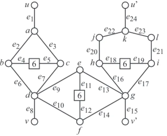
Definition 3. Let u, v, u0, v0 be four distinct vertices linked together according to the structure depicted in Figure 4.8. We assume that all vertices except u, v, u0, v0 in this structure have no additional edges incident to them. Such a structure is called an equalizer for u, v, u0, v0. A simplified representation is also given in Figure 4.8.
Note that an equalizer contains 28 vertices and 39 + 3k edges (since each 6-shift contains 6 vertices and k + 7 edges). We now prove that if k ≥ 12 then the four edges incident to u, v, u0 and v0 necessarily have the same color in every cyclic compact k-edge-coloring of an equalizer. v u Simplified representation 6 6 6 v’ u’ v u v’ u’ e1 e2 e3 e6 e7 e9 e10 e8 e e15 14 e13 e16 e17 e18 e19 e11 e12 e4 e5 e20 e21 e22 e23 e24 a b d c e f g h i j k l
Figure 4.8 An equalizer for u, v, u0, v0.
Lemma 5. Assume k ≥ 12 and let c be a cyclic compact k-edge-coloring of an equalizer for u, v, u0, v0. Then the four edges incident to u, v, u0 and v0 (i.e, edges e1, e8, e15, e24 in
Figure 4.8) have the same color which can be any integer in {0, · · · , k − 1}.
Proof. Let us label the vertices and the edges of the equalizer as in Figure 4.8 and let r be any integer in {0, · · · , k − 1}. We know from Lemma 4 that c(e4) = (c(e5) ± 6)mod k.
Without loss of generality, we can assume that c(e4) = r − 3 and c(e5) = r + 3 (all values are
We first concentrate on vertices u, a, b, c and the 6-shift between b and c. Since b and c are of degree 3, we have c(e2) ∈ [c(e4) − 2, c(e4) + 2]k and c(e3) ∈ [c(e5) − 2, c(e5) + 2]k. In other
words, c(e2) ∈ [r − 5, r − 1]k and c(e3) ∈ [r + 1, r + 5]k. Since the edges incident to a must
have consecutive colors, we necessarily have c(e2) = r − 1, c(e1) = r and c(e3) = r + 1 if
k > 12, while the unique other possibility with k = 12 is c(e2) = r − 5 = r + 7, c(e1) =
r + 6 and c(e3) = r + 5. In both cases, we have {c(e2), c(e3)} = {c(e1) − 1, c(e1) + 1} and
{c(e4), c(e5)} = {c(e1) − 3, c(e1) + 3)}.
Consider now the five edges incident to d. If k > 12, we have c(e6) = r − 2, c(e7) = r + 2
and {c(e8), c(e9), c(e10)} = {r − 1, r, r + 1}. If k = 12, a second possibility is c(e6) = r − 4,
c(e7) = r + 4 and {c(e8), c(e9), c(e10)} = {r + 5, r + 6, r + 7}. In both cases, the colors on
e8, e9 and e10 are consecutive and equal to those on e1, e2, e3.
We can therefore repeat the same reasoning with the subgraph of the equalizer contain-ing vertices v, d, e, f and the 6-shift between e and f . We get {c(e9), c(e10)} = {c(e8) −
1, c(e8) + 1} and {c(e11), c(e12)} = {c(e8) − 3, c(e8) + 3}, which means that c(e8) = c(e1) and
{c(e11), c(e12)} = {r − 3, r + 3}. Also, by considering the five edges incident to g, we get the
same conclusion as for those incident to d : the colors on e15, e16 and e17 are consecutive and
equal to those on e8, e9, e10. By repeating the same reasoning a third and last time on the
subgraph of the equalizer containing vertices v0, g, h, i and the 6-shift between h and i, we get {c(e16), c(e17)} = {c(e15) − 1, c(e15) + 1}, and {c(e18), c(e19)} = {c(e15) − 3, c(e15) + 3)}
which means that c(e15) = c(e8) = c(e1) and {c(e18), c(e19)} = {r − 3, r + 3}.
From {c(e18), c(e19)} = {c(e15) − 3, c(e15) + 3)} and {c(e16), c(e17)} = {c(e15) − 1, c(e15) + 1)},
we deduce {c(e20), c(e21)} = {c(e15) − 2, c(e15) + 2)}. Since vertex k is of degree 3, we
therefore necessarily have {c(e22), c(e23)} = {c(e15)−1, c(e15)+1)}, which means that c(e24) =
c(e15).
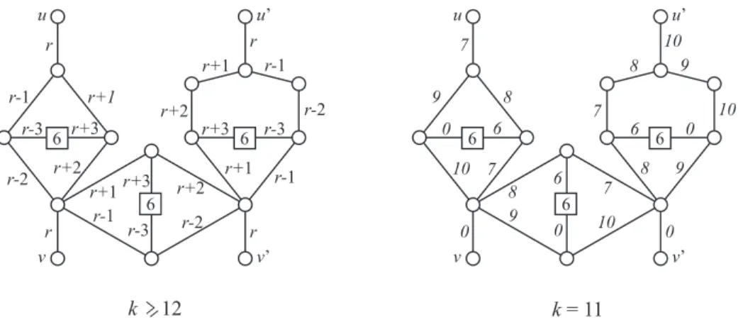
Two cyclic compact k-edge-colorings of the equalizer are depicted in Figure 4.9. The first coloring is valid for all k ≥ 12 while the second coloring demonstrates that the assumption k ≥ 12 is important. Indeed, a cyclic compact 11-edge-coloring is shown with three different colors on e1, e8, e15, e24.
Lemma 6. Assume k ≥ 12, let e and e0 be two non adjacent edges in a graph G, and let G0 be the graph obtained from G by removing e and e0 and adding an equalizer for the four endpoints of these two edges. Then G0 is k-cyclically compactly colorable if and only if G admits a cyclic compact k-edge-coloring c with c(e) = c(e0).
Proof. Let c0 be a cyclic compact k-edge-coloring of G0 and let r be the color on the four edges of the equalizer incident to the endpoints of e and e0. By coloring e and e0 with color
v u 6 6 6 v’ u’ r-1 r+1 r r+3 r-3 r-2 r+2 r r+1 r-1 r+3 r-3 r+2 r-2 r r+1 r-1 r+3 r-3 r+2 r-2 r+1 r-1 r v u 6 6 6 v’ u’ 9 8 7 6 0 10 7 0 8 9 6 0 7 10 0 8 9 6 0 7 10 8 9 10 k = 11 k 12
Figure 4.9 Two k-cyclic compact edge-colorings of an equalizer for u, v, u0, v0.
r and every other edge of G as in G0, one gets a cyclic compact k-edge-coloring c of G with c(e) = c(e0).
On the opposite, let c be a cyclic compact k-edge-coloring of G with c(e) = c(e0). By coloring the edges of the equalizer as in the left graph of Figure 4.9, with r = c(e), and every other edge of G0 as in G, one gets a cyclic compact k-edge-coloring of G0.
We now complete the description of the polynomial time reduction from the k − LCCP to the k − CCCP for k ≥ 12. We denote T (G) the graph obtained from GB+ by removing
the edges eB
i and eHi (i = 1, · · · , t) and replacing them by an equalizer for vi, vi0, ui, wi . A
summary of the transformation is shown in Figure 4.10.
k-|Evi|-1 k-2 k-|Evi+1|-1 vi v’i vi+1 v’i+1 ui wi ui+1 wi+1 Evi Evi+1 Figure 4.10 Illustration of T (G).