Science Arts & Métiers (SAM)
is an open access repository that collects the work of Arts et Métiers Institute of
Technology researchers and makes it freely available over the web where possible.
This is an author-deposited version published in:
https://sam.ensam.eu
Handle ID: .
http://hdl.handle.net/10985/8480
To cite this version :
Abdérafi CHARKI, Khadim DIOP, Stéphane CHAMPMARTIN, Abdelhak AMBARI - Numerical
simulation and experimental study of thrust air bearings with multiple orifices - International
Journal of Mechanical Sciences - Vol. 72, p.28-38 - 2013
Any correspondence concerning this service should be sent to the repository
Administrator :
[email protected]
Numerical simulation and experimental study of thrust air bearings
with multiple orifices
A. Charki
a,n, K. Diop
a, S. Champmartin
b, A. Ambari
baUniversity of Angers, ISTIA-LASQUO, 62 av. Notre Dame du Lac, 49000 Angers, France bENSAM Angers, LAMPA, 2 bd. du Ronceray, 49035 Angers, France
a r t i c l e i n f o
Article history: Received 11 May 2012 Received in revised form 13 October 2012 Accepted 8 March 2013 Available online 20 April 2013 Keywords:
Thrust air bearing Finite element method Experimental study Dynamic analysis
a b s t r a c t
The objective of this paper is to provide a numerical simulation and an experimental study in order to assess stiffness and damping characteristics of thrust air bearings with multiple orifices. Finite element modeling is used to solve the non-linear Reynolds equation while taking into account the movement equation for the bearing. The numerical results obtained show that performance characteristics are related to bearing design type. An experimental investigation allows us to analyze the behavior of thrust air bearings with several orifices as well as that of groove or porous material bearings. Frequency response measurements have been realized in order to compare the dynamic properties of the different bearings. The frequency responses obtained demonstrate that air bearings with multiple orifices have a damping higher than the other types in certain conditions. Air bearings with multiple orifices offer many advantages from a dynamic point of view. Their performance may be characterized not only by flow conditions but also by the number or diameter of the orifices in the bearing surface.
&2013 Elsevier Ltd. All rights reserved.
1. Introduction
The usual approach to the design of thrust air bearings is based on static characteristics. However, when integrated into a system, for instance a spindle or a metrology stage, bearings are subject to load variations, pressure fluctuations or gap variations induced by surface flaws in the slideways. These effects induce excitations of the bearing dynamic response, which can eventually lead to bearing instability. Consequently, the prediction of dynamic char-acteristics in working conditions is necessary for the applications requiring high precision movements or positioning with micro-meter to nanomicro-meter repeatability.
Several approximate analytical approaches to the dynamic behavior of thrust air bearings have been presented in the literature. Licht et al.[1]and Bassani et al.[2]developed analytical models to examine the influence of geometric parameters on the stability of aerostatic bearings with recesses. Their common conclusion is to minimize the depth of the pockets in order to avoid the effect of pneumatic hammer. Stifller [3] conducted a theoretical analysis of a thrust bearing with inherently compen-sated orifices by using a small perturbation of the Reynolds equation, and found that an unstable range occurs when stiffness is at maximum.
Few authors studied numerically the dynamic characteristics of thrust air bearings. Lin et al. [4] proposed a finite element modeling to calculate the static and dynamic characteristics of air bearings using the Gross form of the Reynolds equation [5].
They employed the Runge–Kutta method to solve the coupled
dynamic equation of a journal bearing with shaft, and simulate a thrust pocket bearing to analyze the stable and unstable states for different pocket depths. Fourka et al.[6]established a comparison of the stability map of pocket bearings obtained by finite element modeling. Their findings demonstrated that the analytical method underestimates the critical threshold, giving a wider margin. The same conclusion established by [1,2] is arrived at in [4,6] using FEM to examine the influence of the volume of bearing recess.
Aguirre et al. [7] proposed a new theoretical approach for analyzing the behavior of aerostatic bearings to avoid a self-excited vibration known as pneumatic hammer. They developed a system with the active compensation using air bearings in order to control its position and to reduce the influence of disturbance forces.
Nishio et al.[8] studied numerically and experimentally aero-static annular thrust bearings with feedholes of less than 0.05 mm in diameter. It was confirmed that aerostatic thrust bearings with small feedholes have a larger stiffness and a higher damping coefficient than bearings with compound restrictors.
Bhat et al. [9] analyzed the static and dynamic characteristics of inherently compensated orifice based flat pad air bearing system. The steady state characteristics are studied theoretically and experimentally for a single orifice air bearing. They found that 0020-7403/$ - see front matter & 2013 Elsevier Ltd. All rights reserved.
http://dx.doi.org/10.1016/j.ijmecsci.2013.03.006
n
Corresponding author. Tel.: +33 2 41 22 65 37; fax: +33 2 41 22 65 00. E-mail address: abderafi[email protected] (A. Charki).
pneumatic hammer instability tends to occur at low perturbation frequencies at small orifice diameters (less than 0.25 mm), large gap heights (greater than 20 mm) and large supply pressures.
Boffey [10–14] tested and analyzed the static and dynamic
characteristics of thrust bearings with a pocketed orifice and inherent orifice compensation. The effect of geometric parameters on stability has been shown for pocketed thrust bearings. The same tendencies as those described by [6,10–18] have been deduced from experimental investigations. Nevertheless, few experimental results report the dynamic behavior of thrust air bearings with multiple inherent orifices.
The numerical study using the finite element method pre-sented in this paper allows the analysis of the damping of thrust air bearings fed with multiple orifices. Simulations have been performed in order to describe the influence of geometrical parameters and static equilibrium conditions. The numerical results show that an optimum position may be achieved. The same approach is used by Charki et al. [19] for studying the dynamic behavior of hemispherical air bearings.
An experimental setup is also proposed in this paper. Experi-mental tests have been conducted to compare thrust air bearings with different types of inlet by exciting the bearing system with a variable force around its static equilibrium position. The aim of these experiments is to establish a comparison between porous wall bearings and bearings with orifices of different diameters, both with and without grooves. Frequency response measure-ments are then used to characterize several design types of bearings. The effects of geometrical parameters and of air flow conditions have been investigated.
2. Modeling
2.1. Finite element modeling of a thrust air bearing
In this section, a finite element model is developed for thrust air bearings in order to study the effect of several design and working parameters on fluid film gap characteristics, such as discharge coefficient, supply pressure, number and diameter of orifices and position of orifice rows, and external load.
After introducing the dimensionless variables
p ¼ p Pat ; x ¼ x R2 ; y ¼ y R2 ; h ¼ h h0 ; τ¼ υt;
Patis the atmospheric pressure, υ is the frequency, R2is the outer
radius of the bearing, h is the film gap, h0 is the reference film
gap—with the isothermal perfect gas assumption, the Reynolds equation of compressible flow becomes[5,19–21]
∇:ðh3p∇p−ΛphÞ ¼ s∂ðphÞ∂τ ; ð1Þ
where Λ is the compressibility vector and s is the squeeze parameter [5,19–21]. The components of the compressibility vector in each directions and the squeeze parameter are
respectively expressed as Λx¼ 6μuxR2 h20pat ; Λz¼ 6μuzR2 h20pat and s¼ 12μυR22 h20pat
ux and uz are the components of the velocity vector of the
film flow.
The problem consists in determining the pressure field pðx; zÞ satisfying the dimensionless Reynolds equation(1)and the mass flow rate conservation.
The film flow is developed along a 2-dimensional surface S as it is shown inFig. 1. The solution is defined over a surface S on which the boundary conditions are given by the pressure along the external boundary Γpof the bearing and the mass flow rate qnin
the film along Γq. The mass flow rate qnin the film is defined by qn¼ ρh U− h
2
12μ∇p !
n ð2Þ
where U is the velocity vector of the film flow in each axis directions, and n is the normal unit vector of the Γq.
By applying the Galerkin weighted residual method[19]to(1), the following integral formulation is obtained as
IðpÞ ¼ Z S −∇δp:ðh3p ∇pÞ þ ∇δp:ðphΛÞ−δps∂ph∂τ ! dS− Z Γq δpqndΓ ð3Þ where qn is deduced from (2).
In order to have a matrix formulation, the domain S (seeFig. 1) is descritized with the linear triangular element T3. Thus, the pressure functions are
pðx; z; τÞ ¼ o Nðx; zÞ4 fpnðτÞg ¼ ∑ 3 i ¼ 1 Niðx; zÞ:piðτÞ δpðx; z; τÞ ¼ o Nðx; zÞ4 fδpnðτÞg ¼ ∑ 3 i ¼ 1 Niðx; zÞ : δpiðτÞ
where N is the shape function for which its coefficients are determined with the nodes coordinates. Then, Eq.(3)becomes
IðpÞ ¼ 〈δpn〉 ∑ ne e ¼ 1 ð½KðpnÞ(efpng þ ½C(ef_png þ fFegÞ $ % ¼ 0 where ½KðpnÞ(e¼− Z Seh 3 N f g o p 4 ∂N ∂x & ' o∂N ∂x4þ ∂N ∂z & ' o∂N ∂z4 ( ) dSe þ Z Seh Nf g o ∂N ∂x 4 Λxþ o ∂N ∂z4 Λz ( ) dSe− Z SesN〈N〉 ∂h ∂τdS e ½C(e¼ Z SeshfNg〈N〉 dS e and fFeg ¼− Z Γe q qnfNg dΓ
Finally, taking into account all elements ne of the discretized
surface, the non-linear algebraic non-stationary equations consti-tutes a matrix relation as
½KðpnÞ(fpng þ ½C(f_png þ fFg ¼ 0 ð4Þ
2.2. Static calculation
The non-linear algebraic equation(4)is first solved using the Newton–Raphson method in order to find the static characteris-tics. The calculation procedure is performed as follows:
1. Perform surface meshing.
2. Provide input parameters and boundary conditions. Input feeding parameters: supply pressure, inlet diameter, discharge
Γq
Γp
coefficient, number of inlets; boundary conditions: initial feeding pressure of fluid film and atmospheric pressure, squeeze and compressibility parameters.
3. Perform static calculations and analyze results: flow rate, pressure distribution, load capacity and stiffness.
The pressure distribution is calculated in taking into account the mass conservation in the flow [6,19]. The solution is deter-mined over a surface on which the boundary conditions are given by the pressure along the external boundary of the bearing (see
Fig. 1) and the mass flow rate (2).
In the bearing with orifices, the dimensionless pressure
pr¼ Pr=Pat (where Pr is orifice outlet pressure ) at the exit
determines the flow rate through the orifice[20], which in turn allows us to examine the influence of feeding parameters on pressure in the fluid film.
From the compressible flow theory through [19,22] a nozzle, under isentropic assumption, the dimensionless air mass flow through each one of the feeding holes is expressed as
q ¼12mℜT h30P2at qo¼ hCs 2 γ−1 Pr Ps $ %2=γ − Pr Ps $ %ðγþ1Þ=γ " # ( )1=2 if Pr Ps≥ 2 γþ 1 $ %ðγ−1Þ=γ and q ¼ hCs 2 γþ 1 $ %ððγþ1Þ=2ðγ−1ÞÞ if Pr Ps ≤ 2 γþ 1 $ %ðγ−1Þ=γ ;
where Ps is the feed supply pressure, and Cs is the feeding
parameter expressed as Cs¼ 12μπdCdPs h20P2at ffiffiffiffiffiffiffiffiffiffi γℜT p ;
where T is the atmospheric temperature at supply conditions, Cdis
the discharge coefficient, d is the orifice diameter, μ is the dynamic viscosity of the fluid, γ is the isentropic index and ℜ is the gas constant.
Powel [23]published that Cd is a variable, which expresses a
function of the pressure ratio Pr=Ps.
As normally considered by many authors, the orifice discharge coefficient is equal around to 0.8 for all flow conditions[22].
The gap and pressure steps chosen are equal to 0.05 mm and 0.0001 bar in order to achieve a very small ratio error and to maintain the conservation of mass flow rate through the orifices and in the air film gap. This aspect is particularly important for a very small gap, i.e. at approximately zero.
The work of the designer consists in determining a compromise between the load capacity and the stiffness of the final choice of bearing.
The dimensionless load capacity and stiffness are calculated respectively using the following expressions:
W ¼ W PatR22 ¼ Z s ðp−1Þ dS ð5Þ K ¼ h0K PatR22 ¼−dW dh ð6Þ 2.3. Dynamic calculation
The dynamic calculation derives from the need to solve the Reynolds equation simultaneously with the equation of motion
[19,20], written as ΔFðτÞ ¼ M €h ð7Þ where M ¼mυ 2h 0 PatR22 ;
m is the mass supported by the bearing, Pat is the atmospheric
pressure, υ is the frequency, R2is the outer radius of the bearing, h0
is the reference film gap. ΔF is the variation of the resultant pressure force: from this may be deduced, firstly, the wall accel-eration, and secondly the velocity and variation of air film gap relative to the equilibrium position, using a variable step Euler scheme:
1. Choice of equilibrium position for dynamic calculation. 2. Input of initial step displacements and velocities for step by
step method.
3. Dynamic calculation of the movement (acceleration, velocity, displacement, pressure and load capacity, etc.).
3. Numerical application
3.1. Test case
In this section, a test case is proposed for comparing results obtained with previous works in the literature. Frêne[24]studied the bearing design presented in Figs. 2 and 3. The bearing for which the load capacity has been calculated is shown with another view inFig. 3, where R1, R2and r respectively show the position of
the orifices and the outer and inner radii.
Numerical calculations are performed with a regular mesh, where the feeding orifices are located at the nodes of the fluid film geometry meshing, as shown Fig. 4. Fig. 5 shows the pressure distribution obtained by the FEM developed in Section 2. As shown in Fig. 5, the pressure is distributed from Pr to Pat. Pr is
calculated using the relations presented in Section 2.2 for all conditions shown inTable 1.
The load capacity is calculated with an analytical approach proposed by Frêne[14]in assuming a simple statical case. The load capacity is also obtained experimentally and numerically using FEM.Fig. 6shows that results are different for each case for a film thickness lower than 15 mm, and are very close for numerical and experimental approaches for a film thickness higher than 15 mm.
3.2. Analysis of the equilibrium position
In this paper, the FEM proposed allows us to study the influence of several design and working parameters on air film gap characteristics, such as discharge coefficient, supply pressure, number and diameter, of orifices and position of orifice rows, and external load.
For this section, the bearing configuration considered is pre-sented inFig. 7and its fixed parameters are listed inTable 2.
The dimensionless load capacity and stiffness calculated versus the dimensionless air film gap are respectively presented in
Figs. 8–10. Results are obtained for Ps¼ 5.105Pa, Cd¼ 0.7, R1/R2¼ 0.8, h0¼ 20 mm, R2¼ 32 mm and ω ¼ 1400 rpm. Inlet R2 R1 r Compressed air
As the figures show, the best working conditions lie within a very small gap range. These are obtained for an air film gap of less than 10 mm for all configurations.
Certain parameters are more sensitive than others. The influ-ence of diameter and the number of orifices is very accentuated. Load capacity increases significantly for a very small air film gap as the number of orifices and orifice diameter increases. The load capacity increase drops off severely when there are 24 orifices. The optimum stiffness is found when the film gap diminishes as the orifice diameter is reduced
3.3. Analysis of dynamic responses
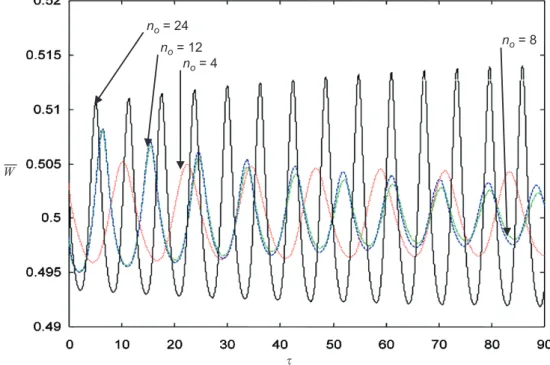
Figs. 11–14 give the dynamic step responses of the bearing
studied above. The results also make it possible to analyze the sensitivity of the parameters vis-à-vis the dynamic behavior of the bearing around an equilibrium position. The step responses are calculated with the Euler scheme as described inSection 2.3, with the same initial conditions: h0¼ 0:5 and _h
0
¼ 0:0.
The dynamic simulations take into consideration two external loads: W ¼ 2:0 and W ¼ 0:5. The dynamic dimensionless air film gap and the load capacity versus dimensionless time are obtained for Ps¼ 5.105Pa, Cd¼ 0.7, R1/R2¼ 0.8, h0¼ 20 mm, R2¼ 32 mm and
ω¼ 1400 rpm. The gap and the pressure step chosen for numerical calculations must be as small as possible for optimal accuracy of results.
For the highest external load W ¼ 2:0, the step responses are not damped for a number of orifices equal to 12 whatever the diameter of orifices as shownFig. 11. The step responses give a higher damped oscillation frequency for a number of orifices equal to 8 or 24.
With an external load equal to 0.5, the damping is increased when the orifice diameter decreases and the number of orifices is equal to 8 or 12 as shown inFigs. 13 and 14. The oscillation amplitude increases considerably for an orifice diameter of 0.6 mm, tending towards a configuration close to an instability range.
Other results obtained by the numerical approach show the same tendency found in the literature [20]. For instance, the influence of the discharge coefficient and of the row position is not significant.
4. Experimentation
4.1. Experimental setup
The experimental setup is presented inFig. 15. The thrust air bearings to be tested are placed on a stable granite base. The block under which the bearing is fixed is supported by a journal air bearing that prevents friction. The static value of the air film gap is measured using a fiber optic sensor with nanometric resolution. The force exerted is measured by a force sensor. The dynamic response of the bearings is analyzed from a small white noise perturbation generated by a shaker controlled by an electrical signal. The frequency response of the bearing is obtained from an accelerometer, using a modal analyzer.
The load is applied at the center of the bearing in order to avoid a parallelism error between bearing surface and support surface. The air flow is filtered by a regulation system to eliminate humidity and solid particles.
4.2. Description of bearings tested
Fig. 16 gives the geometry type of bearings taken into con-sideration in testing, where R2, R1, h, Ps, d, and norespectively are
the outer radius, position of orifice row, reference gap, supply pressure, orifice diameter and number of orifices.Table 3presents the different geometric parameters of all bearings. The groove
d
R2
r R1
Fig. 3. Other view of bearing geometry[24].
Fig. 4. Fluid film meshing.
Pat
Pat Pr
x 1.105 Pa
Fig. 5. Pressure distribution.
Table 1
Thrust bearing parameters of Frêne[24]. Thrust bearing parameters
Outer radius R2(mm) 75
Inner radius r (mm) 30
Reference gap h0(mm) 20
Radius of orifice row R1(mm) 48
Diameter of the feeding orifice d (mm) 0.15
Number of the orifices no 12
Supply pressure Ps(Pa) 3 ) 105
Atmospheric pressure Pat(Pa) 1 ) 105
Coefficient of discharge Cd 0.7
Isentropic index γ 1.4
Gas constant ℜ (J kg-1K−1) 287
Dynamic viscosity μ (Pa s) 18.38 ) 10−6
Temperature at supply conditions T (1K) 293
width of bearing configurations of cases 4 and 5 are respectively equal to 0.2 mm and 0.6 mm. All results shown in following sections are obtained for Ps¼ 5.105Pa, ω¼ 0 rpm and no¼ 8.
Fig. 17 shows another view of the different feeding types of the bearings studied.
Bearing characteristics are dependent on the surface quality obtained from finish diamond machining. For high precision machines or systems, it is very important that the flatness, straightness and roughness of bearing surfaces fall within tight limits. For our purposes, the reference surface flatness is within
1 mm, having been machined by diamond turning. Similarly, the pad surface has been achieved by diamond cutting on the high precision lathe. Furthermore, in order to ensure good parallelism between the surfaces, the holes are drilled to the same diameter and with good roundness. All orifices must be equally spaced
Analytical (Frêne [24])
Experimental Numerical (FEM)
W (N)
h (lm)
Fig. 6. Load capacity versus film gap for Ps¼ 3 bar.
d
R2 R1
Fig. 7. Bearing configuration studied. Table 2
Fixed parameters of thrust bearings studied. Thrust bearing parameters
Outer radius R2(mm) 32
Reference gap h0(mm) 20
Radius of orifice row R1(mm) 25.6
Supply pressure Ps(Pa) 5 ) 105
Atmospheric pressure Pat(Pa) 1 ) 105
Coefficient of discharge Cd 0.7
Isentropic index γ 1.4
Gas constant ℜ (J kg−1K−1) 287
Dynamic viscosity μ (Pa s) 18.38 ) 10−6
Temperature at supply conditions T (1K) 293
Rotational speed ω ¼2πυ (rpm) 1400 W h d = 0.6 mm d = 0.3 mm d = 0.2 mm
Fig. 8. Dimensionless static load capacity versus dimensionless film gap for no¼ 12.
no = 4
no = 8 no = 12
no = 24
Fig. 9. Dimensionless static load capacity versus dimensionless film gap for d¼ 0.2 mm.
along the circumference. The shape of an orifice outlet can be observed inFig. 18.
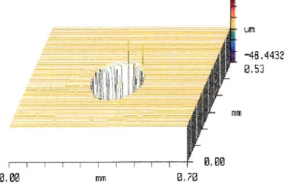
The roughness and form error measurements are made with an interferential microscope and a profilometer comprising a linear stage and an optical fiber sensor, giving a repeatability of less than 0.2 mm for the straightness measurement.Fig. 19shows a rough-ness measurement on the surface of the pad. In order to obtain a high stiffness, the bearings need to work at a very low air film gap, which means that the surface must be free of significant form error waviness.
5. Experimental results
5.1. Testing validity of numerical results
Fig. 20shows that the load capacity W obtained via both the experimental method and a numerical method developed by Bonis and Charki[20]are in good agreement. The experimental results
are obtained using the equipment described in Section 4.1.
A bearing with multiple orifices as shown inFig. 16is tested. Experimental results of W and h shown inFig. 20are based on a mean of six measurements and a respectively standard deviation equal to 10 N and 2 mm. For a very small film gap less than 2 mm, it is difficult to know exactly the maximum load capacity supported by the bearing in order to avoid a solid contact between surfaces of reference support and bearing.
As shown in Fig. 20, two discharge coefficients have been
used in our calculations for the purpose of comparison. The difference in the load capacity relative to the discharge coefficient is very small.
5.2. Dynamic results
The following results serve to investigate the influence of the feeding design on dynamic properties. The frequency responses obtained correspond to the dynamic behavior at the first modal frequency of each bearing. A single supply pressure (5 bar) is considered in order to compare the frequency responses of all the bearing types presented inFig. 17andTable 3.
Fig. 21 illustrates the influence of a groove on the natural frequency and on the amplitude of the frequency response for
W¼35 N and two different diameters (d¼0.2 mm and d¼0.6 mm).
The natural frequency is higher in the presence of a groove; the
d = 0.6 mm d = 0.3 mm
d = 0.2 mm
Fig. 10. Dimensionless stiffness versus dimensionless film gap for no¼ 12.
W
!
d = 0.6 mm d = 0.3 mm d = 0.2 mm
Fig. 11. Dimensionless step response of load capacity versus dimensionless time for W ¼ 2:0 and no¼ 12. W ! no = 4 no = 12 no = 8 no = 24
Fig. 12. Dimensionless step response of load capacity versus dimensionless time for W ¼ 2:0 and d¼0.2 mm. W ! d = 0.6 mm d = 0.2 mm d = 0.3 mm
Fig. 13. Dimensionless step response of load capacity versus dimensionless time for W ¼ 0:5 and no¼ 12.
difference in natural frequency between a bearing with and a bearing without a groove diminishes as the diameter increases, and the amplitude of the responses decreases as the orifice diameter is decreased.
Furthermore,Fig. 22shows that the amplitude of the frequency response diminishes as the load is increased. This aspect is due to the fact that the air film gap decreases, and the acceleration after an excitation reduces. The natural frequency remains almost the same for each load.
The damping ratio ζexp is deduced by means of an empirical
procedure that looks at the amplitude of the frequency response at
W ! no = 8 no = 4 no = 12 no = 24
Fig. 14. Dimensionless step response of load capacity versus dimensionless time for W ¼ 0:5 and d¼0.2 mm.
Power & Charge Amplifiers Pressure transducer Thrust bearing under testing Journal bearing Reference support Granit base Accelerometer Shaker + Load transducer Load
Fiber optical sensor Data acquisition system
Dynamic analysis
Fig. 15. Test rig.
Orifice Ps no R1 d h Surface bearing
Surface reference support
R2
Fig. 16. Geometry bearing tested with multiple orifice.
Table 3
Description of bearings tested.
Geometric parameters Type of feeding
Orifices without groove Orifices with groove
Porous
Case 1 Case 2 Case 3 Case 4 Case 5 Case 6
R2(mm) 32 25 32 32 32 32
R1(mm) 25.6 20 25.6 25.6 25.6 –
d (mm) 0.2 0.2 0.6 0.2 0.6 –
Orifices Orifices + Groove Porous
3 dB [25,26]. The damping ratio ζexp is calculated by using the following expression: ςexp¼f exp 2 −f exp 1 fexpn ð8Þ
where fnexpis the natural frequency corresponding to the top peak
of the frequency response function, f1expand f2expare frequencies
deduced by the half-power bandwidth method [25,26]. The
uncertainty of measurement on ζexpis estimated as
Δςexp¼ 0 0 0 ∂ςexp ∂fexpn 0 0 0Δf exp n þ 0 0 0 ∂ςexp ∂fexp1 0 0 0Δf exp 1 þ 0 0 0 ∂ςexp ∂fexp2 0 0 0Δf exp 2 ð9Þ
where Δfiexp(i ¼ 1,2,n) are the measurement uncertainties of each
frequency. The estimation of Δfiexp(i ¼ 1,2,n)is equal to 3 Hz. This value
of frequency uncertainty takes only into account the experimental standard deviation[27,28] of measurement data samples obtained for all bearings tested.
For each case tested, the natural frequency of the bearing is found to occur at about 100 Hz. As seen inFigs. 22 and 23, struc-tural modes of the test rig are observed at high loads but corres-pond to a much higher frequency, which is easy to distinguish.
Figs. 23 and 24 show the frequency responses of the three bearings, for two loads (W¼135 N and W¼35 N) and an orifice diameter of 0.6 mm. The frequency observed is the same for both loads on each of the bearings and falls within the experimental error range. The amplitude of the frequency responses decreases with an increase in load, demonstrating that the increase in film damping that is generated by an increase of the squeezing effect and of viscous dissipation when the gap height is reduced.
A comparison of the frequency responses of the three types of feeding– orifice, groove, and porous wall with a low permeability (Sika B8)– makes it possible to distinguish clearly between their respective dynamic performances.
In Fig. 23, for the load capacity of 135 N, the acceleration amplitude of the bearing with orifices is lower than for the other bearings, indicating higher damping ratio ζexpat high load, i.e. at small gap. InFig. 24, the trend changes at the lower load of 35 N. In this instance, the bearing with porous material has the lowest acceleration, together with a higher natural frequency (fnexp), and
consequently a higher stiffness, giving it the most preferable dynamic performance among the three types of bearings. The acceleration amplitude of the bearing with groove remains the highest at both loads.
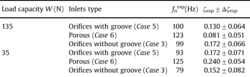
Table 4 presents natural frequencies and damping ratios with uncertainties measurement for two loads (W ¼135 N and Fig. 18. Bearing surface part and hole feed.
Fig. 19. Bearing surface part.
0 5 10 15 20 25 30 35 0 100 200 300 400 Experiment Numerical -Cd = 0.7 Numerical -Cd = 0.9 W (N ) h(lm)
Fig. 20. Load capacity versus air film gap for case 1.
0 200 400 600 800 1000 1200 0 0.5 1 1.5 2 2.5 3 Hz Amp. (m/s2/N) Case 5 Case 3 Case 4 Case 1
Fig. 21. Frequency responses measurement for bearings with and without groove for W¼ 35 N. 0 200 400 600 800 1000 1200 0 0.5 1 1.5 2 2.5 3 Hz Amp. (m/s2/N) W = 135 N W = 85 N W = 35 N
Fig. 22. Frequency responses for bearing without groove for different loads W and for case 2.
W¼35 N) and all different bearings tested as shown in Figs. 23 and 24.
It has been clearly demonstrated that for a very small air film gap, bearings with orifices offer advantages due to their dynamic responses. Bearings may be less subject to perturbations if the orifice diameter chosen is optimal in order to avoid pneumatic hammer. Experiments show that it is possible to improve the dynamic behavior by changing the type of bearing feed.
Fig. 25 gives the numerical results of the bearing with orifices tested Case 3. In Table 5, the damping ratio ζ and the natural frequency fnhave been calculated with the logarithmic decrement
method [25,26]. Numerical results show the same tendencies found in the experimental investigation concerning the natural frequency whereas the damping ratios found are relatively higher.
6. Conclusion
This paper proposes a numerical and experimental approach for analyzing the dynamic response around an equilibrium posi-tion of a bearing with multiple orifices. Calculaposi-tions based on finite element modeling are a means of optimizing the design of a bearing for high precision machines or systems, and take into account different geometrical configurations.
Numerical results obtained show that dynamic characteristics change with feeding conditions. Decreasing the orifice diameter and the air film gap improves the damping of air bearings with a number of orifices equal to 8. With a small load capacity, the oscillation amplitude increases considerably in increasing the orifice diameter, tending towards a configuration close to an instability range.
A comparison between a bearing with orifices and bearings either with a groove or made from porous material is carried out using frequency response measurements. Experimental results show that the bearing with orifices is better damped than the other types for the highest load capacity.
Designers have to pay attention for optimizing the number and the diameter of orifices in accordance to their needs in terms of static and dynamic characteristics. Air bearings with multiple orifices have a good stability but this analysis is correct in certain conditions. 0 200 400 600 800 1000 1200 0 0.2 0.4 0.6 0.8 1 1.2 Hz Amp. (m/s2/N) Porous (Case 6)
Orifices + Groove (Case 5)
Orifices (Case 3)
Fig. 23. Frequency responses for different types of bearings for W ¼ 135N.
0 200 400 600 800 1000 1200 0 0.5 1 1.5 2 2.5 3 frequency (Hz) Amp. (m/s2/N) Porous (Case 6)
Orifices + Groove (Case 5)
Orifices (Case 3)
Fig. 24. Frequency responses for different types of bearings for W ¼35 N.
Table 4
Experimental natural frequencies and damping ratios.
Load capacity W (N) Inlets type fnexp(Hz) ζexp7Δζexp
135 Orifices with groove (Case 5) 100 0.13070.064
Porous (Case 6) 123 0.081 70.051
Orifices without groove (Case 3) 99 0.17270.066
35 Orifices with groove (Case 5) 93 0.17270.071
Porous (Case 6) 125 0.24070.054
The numerical approach developed in this paper allows designers to optimize suitably air bearings with multiple orifices.
List of symbols
p(x,y) pressure field
Pa atmospheric pressure
Ps supply pressure
Pr orifice outlet pressure
R2 outer radius of the bearing
R1 position radius of the orifices
r inner radius d orifice diameter h film gap h0 reference film gap Λ compressibility vector s squeeze parameter υ frequency ω rotational speed
q mass flow rate at the bearing inlet
S surface of the fluid film
Γq, ΓP boundary of the fluid film
n normal vector of the film fluid
N shape function
Cs feeding parameter
T atmospheric at supply conditions
Cd discharge coefficient
no number of orifices
μ dynamic viscosity of the fluid
γ isentropic index
ℜ gas constant
m mass supported by the bearing
W load capacity
K stiffness
τ dimensionless time
ζexp damping ratio obtained experimentally
fnexp natural frequency obtained experimentally
ζ damping ratio obtained numerically
fn natural frequency obtained numerically
References
[1] Licht L, Elrod H. A study of the stability of externally pressurized gas bearings. J Appl Mech 1960:250–8 June.
[2] Bassani R, Ciulli E, Forte P. Pneumatic stability of the integral aerostatic bearing: comparison with other types of bearing. Tribol Int 1989;22(No. 6):363–74 December.
[3] Stiffler AK. Analysis of the stiffness and damping of an inherently compen-sated, multiple-inlet, circular thrust bearing. J Lubr Technol 1974:329–36 July.
[4] Lin G, Aoyama T, Inasaki I. A computer simulation method for dynamic and stability analyses of air bearings. Wear 1988;126:307–19.
[5] Gross AA. Gas film lubrication. New York: Wiley; 54–83.
[6] Fourka M, Tian Y, Bonis M. Prediction of the stability of air thrust bearings by numerical, analytical and experimental methods. Wear 1996;198:1–6. [7] Aguirre G, Al-Bender F, Van Brussel H. A multiphysics model for optimizing
the design of active aerostatic thrust bearings. Precision Eng 2010;34:507–15. [8] Nishio U, Somaya K, Yoshimoto S. Numerical calculation and experimental verification of static and dynamic characteristic of aerostatic thrust bearings with small feedholes. Tribol Int 2011;44:1790–5.
[9] Bhat N, Kumar S, Tan W, Narasimhan R, Low TC. Performance of inherently compensated flat pad aerostatic bearings subject to dynamic perturbation forces. Precision Eng 2012;36:399–407.
[10] Boffey DA. Experimental investigation into the performance of an aerostatic industrial thrust bearing. Tribol Int 1985;18(No. 3):165–8 June.
[11]Boffey DA. An experimental investigation of the effect of orifice restrictor size on the stiffness of an industrial air lubricated thrust bearing. Tribol Int 1981:287–91 October.
[12]Boffey DA. An experimental investigation of the pressures at the Edge of a gas bearing pocket. J Lubr Technol 1981;103:593–600 October.
[13] Boffey DA. An experimental investigation into the rubber-stabilisation of an externally-pressurized air-lubricated thrust bearing. J Lubr Technol 1980;120:65–70 January.
[14] Boffey DA. A study of the stability of an externally pressurized gas lubricated thrust bearing with a flexible damped support. J Lubr Technol 1978;100:364–8 July.
[15] Licht L, Elrod H. A study of the stability of externally pressurized gas bearings. J Appl Mech 1960:250–8 June.
[16] Bassani R, Ciulli E, Forte P. Pneumatic stability of the integral aerostatic bearing: comparison with other types of bearing. Tribol Int 1989;22(No. 6):363–74 December.
[17] Stiffler AK. Analysis of the stiffness and damping of an inherently compen-sated, multiple-inlet, circular thrust bearing. J Lubr Technol 1974:329–36 July.
[18] Lin G, Aoyama T, Inasaki I. A computer simulation method for dynamic and stability analyses of air bearings. Wear 1988;126:307–19.
[19] Charki A, Bigaud D, Guérin F. Behavior analysis of machines and system air hemispherical spindles using finite element modeling. Ind Lubr Tribol 2013;65(4).
[20] Bonis M, Charki A. Modélisation des caractéristiques statiques et de la stabilité des paliers de butée aérostatiques par la méthode des éléments Finis. Eur J Comput Mech 2001;10:755–67. 0.00 0.01 0.02 0.03 0.04 0.05 0 10 20 30 40 50 60 70 80 90 100 F ilm g a p ( µ m) Time (s) W = 35 N W = 135 N
Fig. 25. Numerical step responses for the bearing tested case 3.
Table 5
Numerical natural frequencies and damping ratios—case 3.
Load capacity W (N) Inlets type fn(Hz) ζ 7Δζ
135 Orifices without groove 105 0.10170.041
[21]Charki A, Elsayed EA, Bigaud D, Guérin F. Fluid thrust bearing reliability analysis using finite element modeling and response surface method. Int J Qual Eng Technol 2010;1(No. 2).
[22]Neves MT, Schwarz VA, Menon GJ. Discharge coefficient influence on the performance of aerostatic journal bearings. Tribol Int 2010;43:746–51.
[23]Powell JW. Design of aerostatic bearings. The Machinery Published Co. Ltd; 1970.
[24] Frêne J. Régimes d'écoulement non laminaire en film mince—Application aux paliers lisses, Thèse de Doctorat, Université Claude Bernard de Lyon; 1974.
[25]Thomson WT. Theory of vibration with applications. fourth ed UK: Nelson Thornes; 1993.
[26]〈http://www.xyobalancer.com/_blog/XYO_Balancer_Blog/post/Material_Dam ping_Ratio_Measurement/〉.
[27] Charki A, Louvel D, Renaot , Michel A, Tiplica T. Incertitudes de mesure: applications concrètes pour les étalonnages, Tome 1, EDP Sciences; 2012. [28] Charki A, Gérasimo P, El Mouftari M, Mori Y, Sauvageot C. Incertitudes de
![Fig. 3. Other view of bearing geometry [24].](https://thumb-eu.123doks.com/thumbv2/123doknet/7280739.207379/5.892.82.387.321.791/fig-other-view-of-bearing-geometry.webp)