3 Thèse de Doctorat
Assimilation de données satellitaires pour le suivi des ressources en eau dans la zone Euro-Méditerranée
Daniel Chiyeka SHAMAMBO Décembre 2020
PhD Thesis
Assimilation of satellite data for water resources monitoring over the Euro-Mediterranean area
Daniel Chiyeka Shamambo December 2020
5
Acknowledgements
The three years of working on my thesis project at Centre National de Recherches Météorologique (CNRM) at Météo-France in Toulouse have been a valuable experience for me. Many thanks to Région Occitanie and to Météo-France for funding this project. The successful completion of this PhD project has involved the efforts of many people and I would like to take the opportunity to honor each individual for their contributions.
First and foremost, I am extremely grateful to my supervisors Dr Jean-christophe CALVET and Dr Clément ALBERGEL for all their constant source of guidance, patience, support, inspirations and encouragements during my PhD study. This work would not have been possible had I not have had such excellent supervisors. Their knowledge and experience have encouraged me in all the time during my thesis research project and daily life. I am also grateful to Dr Bertrand BONAN for his scientific and technical support which made this study possible. I also extend my gratitude to Dr. Mehrez ZRIBI and Dr. Jean-Pierre WIGNERON, for their guidance and suggestions as members of my “Comité de Thèse”. I wish to thank my colleagues at Météo-France, particularly at GMME for providing a great research environment. My special thanks go to VEGEO team members for providing a good working environment, constructive discussions and their assistance. Special thanks to Catherine MEUREY for her services in the VEGEO team. I also want to wish Anthony MUCIA, the other PhD student in the VEGEO team all the best for the last phase of his PhD project.
I am thankful to all the staff at CNRM, particularly Anita HUBERT, Ouria GHALAYINI and Régine MANZANO (now retired) for their services and for making my stay at Météo-France a pleasant one.
I would like to acknowledge the Vienna University of Technology (TU Wien) for providing ASCAT σ0 and VOD data and for fruitful discussions. Copernicus Global Land service for LAI data and Copernicus Climate Change Service (C3S) for ERA5 data.
An exceptional thought goes to my parents, my siblings and all the good friends I have met in Toulouse, particularly at ICC and also in France at larger during these years of work and with who I shared both fun and hard times. Last but certainly not least, I would like to express my deep appreciation to Astrid N. for her love and support.
7
Résumé
Une estimation plus précise de l’état des variables des surfaces terrestres est requise afin d’améliorer notre capacité à comprendre, suivre et prévoir le cycle hydrologique terrestre dans diverses régions du monde. En particulier, les zones méditerranéennes sont souvent caractérisées par un déficit en eau du sol affectant la croissance de la végétation. Les dernières simulations du GIEC (Groupe d'Experts Intergouvernemental sur l'Evolution du Climat) indiquent qu’une augmentation de la fréquence des sécheresses et des vagues de chaleur dans la région Euro-Méditerranée est probable. Il est donc crucial d’améliorer les outils et l’utilisation des observations permettant de caractériser la dynamique des processus des surfaces terrestres de cette région. Les modèles des surfaces terrestres ou LSMs (Land Surface Models) ont été développés dans le but de représenter ces processus à diverses échelles spatiales. Ils sont habituellement forçés par des données horaires de variables atmosphériques en point de grille, telles que la température et l’humidité de l’air, le rayonnement solaire et les précipitations. Alors que les LSMs sont des outils efficaces pour suivre de façon continue les conditions de surface, ils présentent encore des défauts provoqués par les erreurs dans les données de forçages, dans les valeurs des paramètres du modèle, par l’absence de représentation de certains processus, et par la mauvaise représentation des processus dans certaines régions et certaines saisons. Il est aussi possible de suivre les conditions de surface depuis l’espace et la modélisation des variables des surfaces terrestres peut être améliorée grâce à l’intégration dynamique de ces observations dans les LSMs. La télédétection spatiale micro-ondes à basse fréquence est particulièrement utile dans le contexte du suivi de ces variables à l’échelle globale ou continentale. Elle a l’avantage de pouvoir fournir des observations par tout-temps, de jour comme de nuit. Plusieurs produits utiles pour le suivi de la végétation et du cycle hydrologique sont déjà disponibles. Ils sont issus de radars en bande C tels que ASCAT (Advanced Scatterometer) ou Sentinel-1. L’assimilation de ces données dans un LSM permet leur intégration de façon cohérente avec la représentation des processus. Les résultats obtenus à partir de l’intégration de données satellitaires fournissent une estimation de l’état des variables des surfaces terrestres qui sont généralement de meilleure qualité que les simulations sans assimilation de données et que les données satellitaires elles-mêmes. L’objectif principal de ce travail de thèse a été d’améliorer la représentation des variables des surfaces terrestres reliées aux cycles de l’eau et du carbone dans le modèle ISBA grâce à l’assimilation d’observations de rétrodiffusion radar (σ°) provenant de l’instrument ASCAT. Un opérateur d’observation capable de représenter les σ° ASCAT à partir de variables simulées par le modèle ISBA a été développé. Une version du WCM (water cloud model) a été mise en œuvre avec succès sur la zone Euro-Méditerranée. Les valeurs simulées ont été comparées avec les observations satellitaires. Une quantification plus détaillée de l’impact de divers facteurs sur le signal a été faite sur le sud-ouest de la France. L’étude de l’impact de la tempête Klaus sur la forêt des Landes a montré que le WCM est capable de représenter un changement brutal de biomasse de la végétation. Le WCM est peu efficace sur les zones karstiques et sur les surfaces agricoles produisant du blé. Dans ce dernier cas, le problème semble provenir d’un décalage temporel entre l’épaisseur optique micro-ondes de la végétation et l’indice de surface foliaire de la végétation. Enfin, l’assimilation directe des σ° ASCAT a été évaluée sur le sud-ouest de la France.
8
Abstract
More accurate estimates of land surface conditions are important for enhancing our ability to understand, monitor, and predict key variables of the terrestrial water cycle in various parts of the globe. In particular, the Mediterranean area is frequently characterized by a marked impact of the soil water deficit on vegetation growth. The latest IPCC (Intergovernmental Panel on Climate Change) simulations indicate that occurrence of droughts and warm spells in the Euro-Mediterranean region are likely to increase. It is therefore crucial to improve the ways of understanding, observing and simulating the dynamics of the land surface processes in the Euro-Mediterranean region. Land surface models (LSMs) have been developed for the purpose of representing the land surface processes at various spatial scales. They are usually forced by hourly gridded atmospheric variables such as air temperature, air humidity, solar radiation, precipitation, and are used to simulate land surface states and fluxes. While LSMs can provide a continuous monitoring of land surface conditions, they still show discrepancies due to forcing and parameter errors, missing processes and inadequate model physics for particular areas or seasons. It is also possible to observe the land surface conditions from space. The modelling of land surface variables can be improved through the dynamical integration of these observations into LSMs. Remote sensing observations are particularly useful in this context because they are able to address global and continental scales. Low frequency microwave remote sensing has advantages because it can provide regular observations in all-weather conditions and at either daytime or night-time. A number of satellite-derived products relevant to the hydrological and vegetation cycles are already available from C-band radars such as the Advanced Scatterometer (ASCAT) or Sentinel-1. Assimilating these data into LSMs permits their integration in the process representation in a consistent way. The results obtained from assimilating satellites products provide land surface variables estimates that are generally superior to the model estimates or satellite observations alone. The main objective of this thesis was to improve the representation of land surface variables linked to the terrestrial water and carbon cycles in the ISBA LSM through the assimilation of ASCAT backscatter (σ°) observations. An observation operator capable of representing the ASCAT σ° from the ISBA simulated variables was developed. A version of the water cloud model (WCM) was successfully implemented over the Euro-Mediterranean area. The simulated values were compared with those observed from space. A more detailed quantification of the influence of various factors on the signal was made over southwestern France. Focusing on the Klaus storm event in the Landes forest, it was shown that the WCM was able to represent abrupt changes in vegetation biomass. It was also found that the WCM had shortcomings over karstic areas and over wheat croplands. It was shown that the latter was related to a discrepancy between the seasonal cycle of microwave vegetation optical depth (VOD) and leaf area index (LAI). Finally, the direct assimilation of ASCAT σ° observations was assessed over southwestern France.
9
Table of content
Acknowledgements
5Résumé
7Abstract
8Table of context
9List of Figures
13List of Tables
19List of Acronyms
21Introduction Générale
23General Introduction
31Chapter I – Scientific context
39
1 Interactions between terrestrial surfaces and the atmosphere ... 40
2 Modelling land surface processes ... 41
3 Earth observations over land ... 42
3.1 Key milestones in the history of spatial remote sensing over land ... 43
3.2 Monitoring land surface variables from space ... 46
4 Use of Earth observations in land surface modelling ... 50
5 Objectives and work scope ... 54
Chapter II - Methodology
57 1 Observations... 58 1.1 ASCAT σ° observations ... 58 1.2 CGLS LAI ... 62 1.3 VOD ... 62 2 ISBA... 6410
2.2 Main characteristics of the ISBA model ... 66
2.3 Atmospheric forcing and land use ... 69
3 LDAS-Monde... 69
4 Observation operator: the Water Cloud Model ... 72
5 Model calibration ... 75
Chapter III - Using satellite scatterometers to monitor land surface
variables
77
1 Analysis of radar backscatter coefficient simulations obtained from the ISBA model coupled to the Water Cloud Model ... 78
1.1 The Euro-Mediterranean area ... 78
1.2 Implementation of the WCM ... 79
1.3 Parameter Values ... 80
1.4 Performance of the WCM ... 84
1.5 Interpretation of results ... 88
1.6 Conclusions ... 92
2 Detailed analyses of results over southwestern France ... 92
2.1 Interpretation of ASCAT radar scatterometer observations over land: A case study over southwestern France (Shamambo et al. 2019) ... 93
2.2 Can LAI simulated by ISBA be used as a vegetation descriptor when fitting the WCM? 116 2.3 Could other versions of the WCM be used? ... 117
2.4 Could other WCM calibration approaches be used? ... 118
3 Synthesis of Chapter III and conclusions ... 124
Chapter IV - Assimilation of ASCAT σ° into the ISBA land surface model
1251 Introduction ... 126
2 Implementation of the Land Data Assimilation System ... 129
2.1 Datasets and data processing ... 129
2.2 Implementation of the water cloud model (WCM) in the Simplified Extended Kalman Filter (SEKF) ... 129
2.3 Configuration of LDAS-Monde ... 131
3 Results and discussion ... 133
3.1 Model sensitivity to the observations... 133
3.2 Impact of the WCM sensitivity to the assimilation on LAI ... 137
3.3 Overall performance of the assimilation of ASCAT σ° observations ... 139
11
Chapter V - Prospects for future use of C-band radar observations
149
1 Introduction ... 150
2. Datasets ... 151
2.1 Vegetation Optical Depth (VOD) ... 151
2.2 LAI Observations ... 151
3. Results and discussion ... 151
3.1. Time series analysis ... 151
3.2 Relationship between LAI/VOD and LAI for straw cereals ... 155
4. Conclusions ... 155
ChapterVI – Conclusions et perspectives
157Chapter VII – Conclusions and prospects
16113
List of Figures
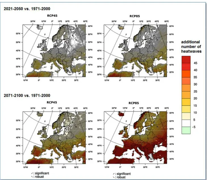
Figure i.1 – Changement du nombre moyen de vagues de chaleur de mai à septembre sur la zone
Euro-Méditerranée pour (en haut) 2021-2050 et pour (en bas) 2071-2100, par rapport à la période 1971-2000, à partir des simulations des modèles climatiques régionaux de l’initiative EURO-CORDEX pour deux scenarios climatiques (Representative Concentration Pathway (RCP) 4.5 et RCP 8.5, à gauche et à droite, respectivement). Les vagues de chaleur sont définies comme des périodes de plus de 3 jours consécutifs dépassant le percentile 99 du maximum journalier de la température de l’air de mai à septembre pour la période 1971- 2000. Le RCP 4.5 est un scénario intermédiaire et le RCP 8.5 est le pire des cas. Adapté de Jacob et al.
(2014). 24
Figure i.2 – Intégration d’observations dans un modèle en utilisant l’assimilation de données (adapté de
http://www.crm.math.ca/crm50/activites/activites-2019/assimilation-de-donnees/) 25
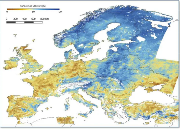
Figure i.3 – Moyenne en août 2018 de l’indice d’humidité superficielle du sol sur l’Europe à une resolution
spatiale de 1 km × 1km telle que dérivée de la combinaison des données en bande C du diffusiomètre ASCAT à basse résolution et du radar à synthèse d’ouverture (SAR) de Sentinel-1 (https://land.copernicus.eu/global/content/first-1km-soil-water-index-productsover-europe, dernier accès en septembre 2020), Bauer-Marschallinger et al. 2018.
26
Figure i.4 – Vue analytique des sujets d’étude abordés dans ce travail 28
Figure i.5 – Change in the mean number of heatwaves from May to September over the Euro-Mediterranean
area for (top) 2021-2050 and for (bottom) 2071-2100, with respect to the 1971- 2000 time period, as simulated by EURO-CORDEX regional climate models for two climate scenarios (Representative Concentration Pathway (RCP) 4.5 and RCP 8.5, left and right, respectively), with heatwaves defined as periods of more than 3 consecutive days exceeding the 99th percentile of the daily maximum temperature of the May to September season for the control period (1971–2000). RCP 4.5 and RCP 8.5 are intermediate and worst-case scenarios, respectively. Adapted from Jacob et al. (2014). 32
Figure i.6 – Integration of observations into a model using data assimilation (http://www.crm.math.ca/crm50/activites/activites-2019/assimilation-de-donnees/)
33
Figure i.7 – Mean surface soil moisture index in August 2018 over Europe at a spatial resolution of 1 km ×
1km as derived from the combination of C-band low resolution ASCAT scatterometer and high resolution Sentinel 1 synthetic aperture radar (SAR) observations (https://land.copernicus.eu/global/content/first-1km-soil-water-index-products-over-europe, last access September 2020), Bauer-Marschallinger et al. 2018. 34
Figure i.8 – Analytic view of the topics addressed in this work. 36
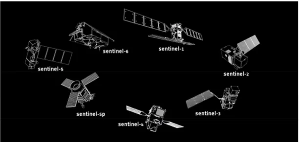
Figure I.1 – Sentinel satellites of the Copernicus space program
(https://gisgeography.com/sentinel-satellites-copernicus-programme/, last access September 2020). 45
Figure I.2 – Reflectance of diverse plant canopies in the visible (VIS), near-infrared (NIR), and shortwave
infrared (SWIR) wavelength bands (https://science.nasa.gov/ems/08_nearinfraredwaves, last
14
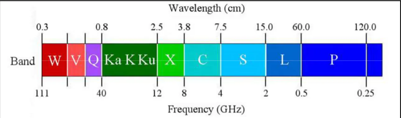
Figure I.3 – Microwave frequency bands (adapted from Ouchi 2013). 48
Figure I-4 – Active and passive microwave sensors used for the generation of the ESA CCI soil moisture
data sets (https://www.esa-soilmoisture-cci.org, last access in September 2020). 49
Figure II.1 – ASCAT swath geometry for Metop A (adapted from Bartalis 2009). 61
Figure II.2 – Schematic representation of the SURFEX modeling platform (adapted from Masson et al.
2013). 65
Figure II.3 – Summary of the “NIT” option of the ISBA model in SURFEX, able to simulate interactive
LAI, herbaceous above-ground biomass, and drought–avoiding and –tolerant responses to soil water deficit. Net assimilation (An) at the canopy level is calculated, together with stomatal conductance (gs), gross primary production (GPP) and ecosystem respiration. Surface variables include atmospheric CO2 concentration, incoming solar radiation (RG), leaf surface temperature (Ts), and leaf-to-air saturation deficit (Ds). Plant specific model parameters include mesophyll conductance in optimal conditions (gm) at a temperature of 25°C, maximum leaf-to-air saturation deficit (Dmax), the ratio (f0) of internal to external CO2 concentration (the CO2 compensation point in optimal conditions (no soil moisture stress and Ds = 0 g kg-1 ) being subtracted from both values). Specific Leaf Area (SLA) is the ratio of LAI to active biomass within green leaves. Leaf plasticity parameters (e and f) depending on vegetation type control the response of SLA to changes in leaf mass-based
nitrogen concentration (NL). 67
Figure II.4 – Carbon allocation in the ISBA model for herbaceous above-ground green vegetation.
68
Figure II.5 – LDAS-Monde 24 hour assimilation cycle: forecast and analysis of 8 control variables using the
SEKF (adapted from Tall et al. 2019). 71
Figure III.1 – Vegetation of the Euro-Mediterranean area (11°W-62°W, 25°N-75°N): (a) land surface types
derived from CLC2000 and GLC2000 at a spatial resolution of about 1 km × 1 km (adapted from Faroux et al. 2013), (b) dominant vegetation type (either grasslands, crops, forests, or sparse vegetation) at a spatial resolution of 0.5° × 0.5° as derived from ECOCLIMAP II (adapted from Szczypta et al. 2014). 79
Figure III.2 – Data flow of the calibration of the water cloud model (WCM): four parameters are tuned (A,
B, C, D) using the forcing of ASCAT C-band VV σ° observations at an incidence angle of 40°, simulated surface soil moisture (SSM), and leaf area index (LAI) observations.
80
Figure III.3 – WCM parameters: histograms of calibrated values over the 2008–2018 calibration time period
(in red) over Euro-Mediterranean area at a spatial resolution of 25 km × 25 km (representing
59 792 grid cells). 81
Figure III.4 – WCM parameters: calibrated values for 2008−2018 over the EuroMediterranean area of
parameter A. 82
Figure III.5 – WCM parameters: calibrated values for 2008−2018 over the EuroMediterranean area of
parameter B. 82
Figure III.6 – WCM parameters: calibrated values for 2008−2018 over the EuroMediterranean area of
parameter C. 83
Figure III.7 – WCM parameters: calibrated values for 2008−2018 over the EuroMediterranean area of
15
Figure III.8 – WCM performance: (a, b) observed σ° from Advanced Scatterometer (ASCAT)
(sigma0_OBS), (c, d) simulated σ° (sigma0_FIT), (e, f) mean bias (simulations– observations), (g, h) temporal correlation, (i, j) RMSD, for (a, c, e) the March, April, and May (MAM) spring period and for (b, d, f) the June, July, and August (JJA) summer period. All values are averaged or calculated for the period from 2008 to 2018. 85-86
Figure III.9 – WCM performance: σ° simulated by the WCM (red lines and dots) vs. ASCAT σ°
observations (blue lines and dots) over the Euro-Mediterranean area from 2008 to 2018. (a) monthly mean values. (b) Scaled monthly anomalies. 87
Figure III.10 – Plain and mountainous calcareous areas (adapted from Williams and Ford 2006) (in dark
blue) and low-altitude (< 1200 m above sea level) mountainous karstic areas (in red) for which low R values of WCM σ° vs. ASCAT σ° are observed in Figure III.8: from West to East, 1 – Cantabrian mountains, 2 – Baetic and Iberian Systems and Toledo Mountains, 3 – Pyrenees, 4 – Causses, 5 – Jura, 6 – French Alps and Côte d’Azur, 7 – Northern calcareous Alps, 8 – Dinaric Alps, 9 – Carpathians, 10 – Transylvanian Alps, 11 – Southern Greece, 12 – Taurus Mountains, 13 – Caucasus Mountains, 14 – Ural Mountains. 90
Figure III.11 – Example of low-altitude karstic area with limestone outcrops in Côte d’Azur (France, 23 km
north of Cannes). Photo by J.-C. Calvet, May 2018. 90
Figure III.12 – C-band RFI map over the Euro-Mediterranean area produced from Sentinel-1 data by
Monti-Garnieri et al. 2017 (adapted from Fig. 10 in Monti-Monti-Garnieri et al. 2017). 91
Figure III.13 – Dominant land cover classes over France as derived from ECOCLIMAP-II (Faroux et al.
2013) at a spatial resolution of 1 km x 1 km. The southwestern France area investigated in this Section is indicated (dark line). 92
Article–Figure 1 – Southwestern France: study area (a) and location of the “Storm” Landes forest site (b).
“Storm” refers to the forest area most affected by the Klaus storm. “North” and “South” are bordering agricultural areas. Fractional area of the main vegetation types is shown in (c–h),
adapted from Brut et al. 2009. 97
Article–Figure 2 – Flowchart of data and methods used in this study for model calibration. 100
Article–Figure 3 – WCM parameters: histograms of calibrated values over the 2010–2013 calibration period
(in blue) and over the 2010–2016 period (in red) over southwestern France at a spatial resolution of 25 km × 25 km (representing 308 grid cells). 102
Article–Figure 4 – WCM parameters: calibrated values for 2010−2016 over southwestern France. From left
to right and from top to bottom: parameters A, B, C, and D. Areas presenting a mean elevation greater than 1200 m a.s.l. are in white. Geographic landmarks are indicated: (a) “1” and “2” for Toulouse and Bordeaux urban areas, (c,d) “3”, “4”, “5” and “6” for the volcanoes of the Cantal, and for Quercy, Corbières, Cévennes karstic areas, respectively. 102
Article–Figure 5 – WCM performance: (a,b) observed σ° from Advanced Scatterometer (ASCAT)
(sigma0_Obs), (c,d) WCM correlation coefficient scores and (e,f) mean bias (simulations– observations), for (a,c,e) the March, April, and May (MAM) spring period and the June, July, and August (JJA) summer period. All values are averaged from 2010 to 2016. Areas presenting an elevation greater than 1200 m a.s.l are in white. Geographic landmarks are indicated: (a,b) “1” and “2” for the Toulouse and Bordeaux urban areas; (c,d) “4”, “5”, and “6” for the Quercy, Corbières, and Cévennes karstic areas, respectively; and (e,f) “7” and “8” for the Lomagne and Bas-Armagnac (South zone in Figure 1) agricultural areas, respectively.
16
Article–Figure 6 – WCM performance: σ° simulated by the WCM (red lines and dots) vs. ASCAT σ°
observations (blue lines and dots) and over southwestern France from 2010 to 2016. (a) Daily and (b) monthly mean values. (c) Scaled monthly anomalies. 105
Article–Figure 7 – Landes forest Storm area: differences in σ° and leaf area index (LAI) with respect to
bordering agricultural areas. (a) ASCAT σ° observations (blue line), (b) simulated σ° values using the WCM parameters values listed in Table 3 (red line) vs. observations (blue line), (c)
LAI. 106
Article–Figure 8 – Mean monthly Copernicus Global Land Service (CGLS) LAI observations over the
Landes forest area most affected by the Klaus storm before (2007) and after (2009) the storm (purple and green lines, respectively). 107
Article–Figure 9 – Agricultural areas: σ° response to surface soil moisture (SSM) and LAI variables. (a,c)
observed ASCAT σ°, (b,d) simulated σ°, (a,b) Bas-Armagnac (“South” in Figure 1) and (c,d) Lomagne agricultural areas. LAI 0%–20%, 21%–79%, 80%–100% percentile classes are indicated (red dots, blue triangles, and green stars, respectively). 109
Article–Figure 10 – Agricultural areas: observed satellite-derived GEOV2 LAI values from 2010 to 2016
over Bas-Armagnac (“South” in Figure 1) and Lomagne. 109
Figure III.14 – Time-series showing LAI observations from the CGLS GEOV2 satellite-derived product (in
green) and the modelled LAI from the ISBA LSM (in yellow) over (top) the agricultural South zone and (bottom) the Landes forest Storm zone described in Shamambo et al. (2019).
116
Figure III.15 – Histograms of WCM parameters when estimated all at once over 2010- 2016 period (in blue)
and over the 2010-2013 calibration period (in red). Approach 1 as described in Shamambo et al. (2019) is applied over southwestern France with WCM Option 1 (V1 = 1). 122
Figure III.16 – As Figure III.15, except for calibration Approach 2. 122
Figure III.17 – As Figure III.15, except for calibration Approach 3. 123
Figure III.18 – As Figure III.15, except for calibration Approach 4. 123
Figure IV.1 – Location of the 21 SMOSMANIA stations in southern France and the locations over which
data assimilation was tested corresponding to the 12 wersternmost SMOSMANIA stations (within the blue box). Adapted from Zhang et al. 2019. Station full names and soil characteristics can be found in the Supplement of Calvet et al. 2016. 127
Figure IV.2 – ASCAT σ° (sigma0_OBS) observations response to surface soil moisture (SSM) from ISBA
(wg2) and CGLS LAI for (a) CDM (b) PRG (c) LHS and (D) MTM stations. LAI 0%–20%, 21%–79%, 80%–100% percentile classes are indicated (red dots, blue triangles, and green
stars, respectively). 128
Figure IV.3 – Flowchart of data and methods used in this study for model calibration of the WCM (elements
associated with arrows and boxes in red), model simulation (elements associated with arrows and boxes in blue) and SEKF assimilation scheme (elements associated with dashed arrows
and dashed boxes in green). 132
Figure IV.4 – Monthly average seasonal evolution from 2007-2016 over the SBR station of: (a) Jacobians
for LAI (red line), wg2 (green dashed line), wg4 (blue dashed line) and wg6 (yellow dashed line); (b) daily analysis increments for LAI (red line), wg2 (green dashed line), wg4 (blue dashed line) and wg6 (yellow dashed line); (c) analysis minus openloop for LAI variable (red line) (d) analysis minus openloop for wg2 (green dashed line), wg4 (blue dashed line) and
17
Figure IV.5 – As in Figure IV.4, except for the CRD station. 134
Figure IV.6 – As in Figure IV.4, except for the PRG station. 135
Figure IV.7 – As in Figure IV.4, except for the CDM station. 135
Figure IV.8 – As in Figure IV.4, except for the LHS station. 136
Figure IV.9 – As in Figure IV.4, except for the MTM station. 136
Figure IV.10 – Leaf area index time series from the openloop (blue dashed line), the observations (green
dashed line), and the analysis (red line) from 2007 to 2016 for (from top to bottom) the SBR,
CRD, LHS, MTM stations. 138
Figure IV.11 – Leaf area index (LAI) seasonal (a,c,e) RMSD and (b,d,f) R scores of openloop (blue line) and
the analysis (red line) from 2007 to 2016 with respect to CGLS LAI for (a,b) the CRD station, (c,d) the LHS station, (e,f) the MTM station. 143
Figure IV.12 – Surface soil moisture (SSM) seasonal (a,c,e) RMSD and (b,d,f) R scores of openloop (blue
line) and the analysis (red line) from 2007 to 2016 with respect to ASCAT SWI for (a,b) the CRD station, (c,d) the LHS station, (e,f) the MTM station. 144
Figure V.1 – Temporal evolution of (a) VOD, (b) LAI and (c) the ratio of LAI to VOD (LAI/VOD) for year
2010 over a straw cereal crop area in southwestern France close to the Lomagne area in Figure 1 of Shamambo et al. (2019). 153
Figure V.2 – Hysteresis in the LAI/VOD vs. LAI relationship for straw cereal areas: schematic
representations of (a) LAI and VOD temporal evolution (x-axis represents time) and (b) the relationship between LAI/VOD and LAI from (1) leaf onset to (2) peak LAI and to (3)
senescence. 154
Figure V.3 – Hysteresis in the LAI/VOD vs. LAI relationship for straw cereal areas: satellite-derived
observations for April, May and June 2010 over a straw cereal crop area in southwestern France close to the Lomagne area in Figure 1 of Shamambo et al. (2019). 154
19
List of Tables
Table II.1 – The main characteristics of the ASCAT scatterometer. 60
Table III.1 – Water cloud model (WCM) parameters (A, B, C, and D) over the Euro-Mediterranean area:
minimum, median, and maximum values, together with standard deviation and skewness
scores. 81
Table III.2 – WCM performance: statistical scores (R and RMSD) of simulated σ° values over the
Euro-Mediterranean area. The calibration period of the parameters is from 2008 to 2018. The calibration scores are given for the pooled dataset (All) and for the March, April, and May (MAM) spring period and the June, July, and August (JJA) summer period. The total number
of observations is indicated (n). 84
Article–Table 1 – Water cloud model (WCM) parameters (A, B, C, and D) over southwestern France:
minimum, median, and maximum values, together with standard deviation and skewness
scores. 102
Article–Table 2 – WCM performance: statistical scores of simulated σ° values over southwestern France.
The calibration period of the parameters is from 2010 to 2013, and the validation period is from 2014 to 2016. For both calibration and validation periods, scores are given for the pooled dataset (All) and for the March, April, and May (MAM) spring period and the June, July, and August (JJA) summer period. The number of observations is indicated (n).
103
Article–Table 3 – Landes forest Storm area: parameters of the WCM before and after the Klaus storm event
of 24 January 2009. The number of observations is indicated (n). The contrasting value of B for the forest regeneration period is in bold. 106
Article–Table 4 – Agricultural areas: parameters of the WCM for Lomagne and Bas-Armagnac (“7” and “8”
in Figure 5, respectively). The number of observations is indicated (n). The contrasting value of B for Lomagne at springtime is in bold. 108
Table III.3 – WCM option 1 (V1 = 1): Statistical scores for radar backscatter coefficient over the storm zone
for the 2007-2016 time period. 118
Table III.4 – WCM option 2 (V1 = LAI): Statistical scores for radar backscatter coefficient over the storm zone for the 2007-2016 time period. 118
Table III.5 – WCM Option 1 (V1 = 1): Statistical scores from each methodology of calibrating the WCM over southwestern France. The calibration period of the parameters was taken from 2010 to 2013 and validation period was from 2014 to 2016. The parameters used for the Dry and Wet conditions are the same as those coming from the calibration under All conditions.
120
Table III.6 – WCM Option 2 (V1 = LAI): Stastistical scores from each methodology of calibrating the WCM over southwestern France. The calibration period of the parameters was taken from 2010 to 2013 and validation period was from 2014 to 2016. The parameters used for the Dry and Wet conditions are the same as those coming from calibration period of All conditions calibration
20
Table IV.1 – Water cloud model (WCM) parameters (A, B, C, and D) values for the 12 SMOSMANIA
stations in southwestern France and their statistical score (RMSD, R, and mean bias) between simulated and observed σ°, together with the critical surface soil moisture (SSMC) calculated from A, C, and D parameters and in situ observations of the porosity of the top
soil layer (Calvet et al. 2016). 137
Table IV.2 – Statistics (RMSD: root mean square difference, R: correlation, and mean bias) between
LDAS-Monde estimates (open loop, analysis based on the assimilation of ASCAT σ0 with an uncertainty of 0.33 dB) and observations for CGLS true leaf area index (LAI [m2m−2]), and ASCAT Soil Water Index (SSM [m3m−3]) over each SMOSMANIA station examined for the period 2007–2016. Note that for the comparison, ASCAT SWI is converted to Surface Soil Moisture (SSM [m3m−3]) with the same seasonal linear rescaling employed to assimilate ASCAT SWI in LDAS-Monde. Improved (degraded) scores of the analysis with respect to the open-loop are in bold and blue (red). 140-142
Table IV.3 – Correlations between LDAS-Monde estimates (openloop, analysis) and in situ measurements
from the SMOSMANIA network over the period 2007 – 2016. Improved (degraded) scores of the analysis with respect to the open-loop are in bold and blue (red). 146
Table IV.4 – Anomaly correlations between LDAS-Monde estimates (openloop, analysis) and in situ
measurements from the SMOSMANIA network over the period 2007 – 2016. Improved (degraded) scores of the analysis with respect to the open-loop are in bold and blue (red).
21
List of Acronyms
AMSR-E Advanced Microwave Scanning Radiometer for EOS
GLDAS Global Land Data Assimilation System
ASCAT Advanced Scatterometer GPP Gross Primary Production ASTER Advanced Spaceborne Thermal
Emission and Reflection Radiometer
HSAF Hydrology Satellite Application Facility
AVHRR Advanced Very High Resolution Radiometer
IAP94 Institute of Atmospheric Physics BATS Biosphere-Atmosphere Transfer
Scheme
ISBA Interaction between Soil-Biosphere-Atmosphere
CCDAS Carbon Cycle Data Assimilation System
IBIS Integrated Biosphere Simulator model
CCE Competitive Complex Evolution IPCC Intergovernmental Panel on Climate Change
CDF Cumulative Distribution Function ISBA Interactions between Soil, Biosphere, and Atmosphere CGLS Copernicus Global Land Service JJA June–July–August
CLM Community Land Model JULES Joint UK Land Environment Simulator
CLVLDAS Coupled Land Vegetation LDAS LAI Leaf Area Index
CNES Centre National d'Etudes Spatiales LDAS Land Data Assimilation System CNRM Centre National de Recherches
Météorologiques
LSM Land Surface Model CTRIP CNRM-Total Runoff Integrating
Pathways
LSV Land Surface Variables CYCLOPES Carbon cYcle and Change in Land
Observational Products from an Ensemble of Satellites
MAM March–April–May
ECMWF European Centre for Medium-Range Weather Forecasts
MCMC Markov Chain Monte Carlo
ECVs Essential Climate Variables METOP Meteorological Operational Satellite ECUME Exchange Coefficients from Unified
Multicampaigns Estimates
MERIS MEdium Resolution Imaging Spectrometer
Eos Earth observations MODIS Moderate Resolution Imaging Spectroradiometer
EnKF Ensemble Kalman filter MOSES Met Office Surface Exchange Scheme
ERA-5 ECMWF Reanalysis 5th generation MSI Multispectral instruments ERS European Remote Sensing MSS Multi Spectral Scanner ERTS Earth Resources Technology
Satellite
NASA National Aeronautics and Space Administration
ESA European Space Agency NCA-LDAS National Climate Assessment-Land Data Assimilation System
ETM Enhanced Thematic Mapper NDVI Normalized Difference Vegetation Index
EUMETSAT European Organization for the Exploitation of Meteorological Satellites
NIR Near infrared
EURO-CORDEX
Coordinated Downscaling Experiment - European Domain
NOAA National Oceanic and Atmospheric Administration
22 EVI Enhanced Vegetation Index NSCAT NASA Scatterometer
FAPAR Fraction of the Photosynthetically Active Radiation absorbed by vegetation
NWP Numerical Weather Prediction
FEWS NET Famine Early Warning Systems Network
RFI Radio Frequency Interference FCOVER Fraction of vegetation cover PILPS Project for Intercomparison of
Landsurface Parameterisation Schemes
GCM Global Climate Models VV Vertical polarization
GLC Global Land Cover SMOS Soil Moisture and Ocean Salinity PROBA-V Project for On-Board Autonomy—
Vegetation
SMOS-MANIA
Soil Moisture Observing System – Meteorological Automatic Network Integrated Application
OLCI Ocean and Land Colour Instrument SMMR Scanning Multichannel Microwave Radiometer
ORCHIDEE Organising Carbon and Hydrology in Dynamics Ecosystems
SNSB Swedish National Space Board RADSCAT RadiometerScatterometer SSM Surface Soil Moisture
RBV Return Beam Vidicon SSTC Scientific, Technical and Cultural Services
RCP Representative Concentration Pathway
SURFEX Surface Externalisée (externalized surface models)
RMSD Root Mean Square Deviation SWIR Short Wave Infrared SAR Synthetic Aperture Radar TEB Town Energy Balance SCE-UA Shuffled Complex Evolution
Algorithm
TIROS-1 Television Infrared Observation Satellite
SEKF Simplified Extended Kalman Filter TM Thematic Mapper
SDD Standard deviation VCI Vegetation Condition Index SiB Simple Biosphere Model VIS visible
SIF Solar Induced Fluorescence VOD Vegetation Optical Depth SLA Specific Leaf Area VPI Vegetation Productivity Index SPOT System for Earth Observation,
“Système Pour l’Observation de la Terre
VWC Vegetation Water Content
SPOT-VGT Vegetation sensor on SPOT
(‘Système probatoire d’observation de la Terre’ or ‘Satellite pour l’observation de la Terre’) satellite
WCM Water Cloud Model
SMAP Soil Moisture Active Passive NLDAS North American Land Data
Assimilation System
23
Introduction Générale
L’observation de la Terre depuis l’espace existe depuis plus de quarante ans. Elle devient une source de données primordiale pour l’étude du climat et pour la validation des modèles des surfaces terrestres, dans un contexte où les effets du réchauffement climatique sur l’environnement sont de plus en plus visibles. Le GIEC (Groupe d'Experts Intergouvernemental sur l'Evolution du Climat) nous alerte sur la forte probabilité d’un accroissement généralisé des aléas climatiques tels que les sécheresses, vagues de chaleur, précipitations extrêmes, feux de forêts, dans les années et les décennies qui viennent.
Ce constat est particulièrement alarmant pour la zone Euro-Méditerranée. L’initiative EURO-CORDEX (https://www.euro-cordex.net/) a permis d’améliorer les simulations climatiques utilisées par les experts du GIEC sur cette zone grâce à l’utilisation de modèles de climat régionaux. En particulier, la résolution spatiale de ces simulations climatiques est meilleure que les simulations climatiques classiques et peut atteindre 12,5 × 12,5 km. Les résultats de ces simulations climatiques publiés par Jacob et al. (2014) montrent, outre une augmentation de la température de l’air, un changement important dans le régime des précipitations, avec un accroissement en Europe Centrale et en Europe du Nord et une tendance à l’assèchement dans les régions plus proches de la Méditerranée. Ces tendances s’accompagnent d’un accroissement généralisé du nombre d’évènements de précipitations intenses en automne. Un autre résultat de cette étude est l’accroissement considérable au cours du 21ième siècle du nombre de vagues de chaleur, pouvant aller jusqu’à plus de 40 évènements supplémentaires de mai à septembre à la fin du siècle (Figure i.1).
Cette évolution du climat a un impact sur les ressources en eau et sur l’agriculture. Certaines variables des surfaces terrestres permettant de caractériser l’impact du changement climatique sur les écosystèmes naturels et cultivés sont observables depuis l’espace. Il s’agit par exemple de l’indice de surface foliaire de la végétation « vrai » (LAI ou « true leaf area index » en anglais), de l’humidité superficielle du sol, et de l’albédo de surface. Cette dernière caractérise la part de rayonnement solaire réfléchi par la surface. Ces variables présentent une variabilité interannuelle, saisonnière, décadaire, voire journalière. Les données satallitaires ne représentant pas toutes les échelles spatiales et temporelles auxquelles se manifestent les effets du changement climatique, il est important d’associer les observations satellitaires à la modélisation des surfaces terrestres. La modélisation permet de comprendre les processus à l’œuvre à diverses échelles temporelles, d’assurer la cohérence entre variables, et d’accéder à des variables qui ne sont pas directement observables depuis l’espace, comme l’humidité du sol dans la zone racinaire.
L’adaptation au changement climatique est un sujet complexe comprenant de nombreux aspects socio-économiques. Elle doit avoir aussi une composante de suivi du climat et des évènements climatiques extrêmes qui repose sur l’amélioration des systèmes d’observation et des systèmes d’alerte. L’observation spatiale a un rôle important à jouer dans la mise en œuvre d’un suivi des surfaces terrestres à l’échelle mondiale et aussi à
24
l’échelle régionale grâce à des observations à plus haute résolution spatiale. L’évaluation de l’intégration de nouvelles observations dans les modèles des surfaces terrestres est nécessaire dans ce contexte.
Figure i.1 – Changement du nombre moyen de vagues de chaleur de mai à septembre sur la zone Euro-Méditerranée pour (en haut) 2021-2050 et pour (en bas) 2071-2100, par rapport à la période 1971-2000, à partir des simulations des modèles climatiques régionaux de l’initiative EURO-CORDEX pour deux scenarios climatiques (Representative Concentration Pathway (RCP) 4.5 et RCP 8.5, à gauche et à droite, respectivement). Les vagues de chaleur sont définies comme des périodes de plus de 3 jours consécutifs dépassant le percentile 99 du maximum journalier de la température de l’air de mai à septembre pour la période 1971-2000. Le RCP 4.5 est un scénario intermédiaire et le RCP 8.5 est le pire des cas. Adapté de Jacob et al. (2014).
25 Figure i.2 – Intégration d’observations dans un modèle en utilisant l’assimilation de données (adapté de
http://www.crm.math.ca/crm50/activites/activites-2019/assimilation-de-donnees/).
Il existe plusieurs méthodes permettant de fusionner les observations satellitaires et les modèles. La méthode la plus sophistiquée consiste à agir sur la physique du modèle et sur les simulations via l’intégration d’observations satellitaires. Il s’agit de l’assimilation de données (Figure i.2). Cette dernière peut-être utilisée pour déterminer plus précisément la valeur de certains paramètres du modèle ou bien pour corriger la trajectoire du modèle au fil de l’eau.
Le Centre National de Recherches Météorologiques (CNRM) a mis en œuvre un système d’assimilation de données (LDAS ou « land data assimilation system » en anglais) permettant de corriger la trajectoire du modèle ISBA (Interactions Sol-Biosphère-Atmosphère) au fil de l’eau en assimilant des produits satellitaires de LAI et d’humidité superficielle du sol. La mise en œuvre de cet outil à l’échelle mondiale est appelée « LDAS-Monde » (Albergel et al. 2017). Il s’agit d’un outil unique car l’assimilation du LAI permet de faire une analyse du contenu en eau du sol dans la zone racinaire, y compris en conditions sèches lorsque l’assimilation de l’humidité superficielle du sol n’apporte que peu d’information. LDAS-Monde est donc bien adapté au suivi des sécheresses et des vagues de chaleur (Albergel et al. 2019).
Les produits satellitaires assimilés par LDAS-Monde proviennent aujourd’hui du service Copernicus Global Land (https://land.copernicus.eu/global/). Le produit LAI « vrai » est élaboré à partir de données spatiales européennes SPOT-Végétation (Baret et al. 2013), PROBA-V et bientôt Sentinel-3. Le produit d’humidité du sol vient essentiellement des observations du radar diffusiomètre en bande C ASCAT. Il s’agit d’un instument des satellites météorologiques défilants européens METOP. Alors que le produit LAI est
26
disponible sur une période de plus de 20 ans, les données ASCAT ne sont disponibles que depuis 2007. Depuis peu, il existe une variante du produit d’humidité du sol à une résolution spatiale améliorée de 1 km × 1 km grâce aux données du radar à synthèse d’ouverture (« SAR » en anglais) en bande C du satellite Sentinel-1 (Bauer-Marschallinger et al. 2018) comme illustré dans la Figure i.3.
Figure i.3 – Moyenne en août 2018 de l’indice d’humidité superficielle du sol sur l’Europe à une resolution spatiale de 1 km × 1 km telle que dérivée de la combinaison des données en bande C du diffusiomètre ASCAT à basse résolution et du radar à
synthèse d’ouverture (SAR) de Sentinel-1
(
https://land.copernicus.eu/global/content/first-1km-soil-water-index-products-over-europe, dernier accès en septembre 2020), Bauer-Marschallinger et al. 2018.
Les produits satellitaires micro-ondes radar sont aujourd’hui essentiellement utilisés pour caractériser l’humidité du sol. Plusieurs études récentes ont cependant montré que les coefficients de rétrodiffusion radar (σ°) contiennent de l’information potentiellement utile pour caractériser la végétation (par exemple Vreugdenhil et al. 2016) au travers de l’épaisseur optique micro-ondes de la végétation (VOD pour « vegetation optical depth » en anglais). Cette variable VOD est reliée au LAI tout en incorporant d’autres caractéristiques
27
physiologues des plantes en relation avec leur contenu en eau. Un avantage considérable des
σ° en bande C est leur disponibilité par tout temps car le signal est peu affecté par l’atmosphère, les nuages en particulier. Le modèle ISBA permettant de simuler en même temps la croissance de la végétation et la variabilité spatiale et temporelle de l’humidité du sol, il est possible que l’on puisse simuler les σ° en bande C. Si cette condition est remplie, l’assimilation des σ° grâce à l’outil LDAS-Monde devient possible et peut être mise en œuvre en remplacement de l’assimilation de l’humidité superficielle du sol. Dans ce travail de thèse, de longues séries temporelles σ° en bande C issues des observations des instruments ASCAT sont analysées sur la zone Euro-Méditerranée et un opérateur d’observation est construit afin de permettre leur assimilation par le modèle ISBA. Une étude plus détaillée est menée sur le sud-ouest de la France (Shamambo et al. 2019).
Les objectifs de ce travail de thèse sont :
• D’évaluer la faisabilité de simuler les σ° en bande C mesurés par les instruments ASCAT sur les surfaces terrestres à partir de variables pouvant être simulées par le modèle ISBA sur la zone Euro-Méditerranée,
• D’analyser l’influence d’éventuels facteurs perturbateurs du signal,
• De contruire un opérateur d’observation pour l’assimilation des σ° ASCAT par LDAS-Monde,
• D’analyser la répartition spatiale et temporelle des paramètres de l’opérateur d’observation,
• De comprendre la réponse des σ° ASCAT observés et simulés aux variables des surfaces terrestres telles que le LAI et l’humidité superficielle du sol,
• D’explorer la relation entre LAI et VOD, en particulier sur les zones cultivées,
• D’évaluer l’impact d’un changement rapide d’occupation du sol sur le signal en prenant l’exemple de la tempête Klaus de janvier 2009 dans la forêt des Landes,
• De mettre en œuvre l’assimilation des σ° ASCAT par LDAS-Monde et d’évaluer son impact sur les variables simulées par ISBA.
La Figure i.4 résume les questions scientifiques qui ont été à l’origine de ce travail ainsi que la façon dont les objectifs de la thèse ont été atteints.
28 Figure i.4 – Vue analytique des sujets d’étude abordés dans ce travail.
29
L’effort a d’abord porté sur la contruction d’un opérateur d’observation, c’est-à-dire une extension du modèle ISBA lui donnant la possibilité de simuler les observations satellitaires de σ° en bande C. Il s’agit d’une étape indispensable avant de mettre en œuvre l’assimilation de données car le modèle ne peut assimiler que les observations qu’il est capable de représenter. En préalable à l’assimilation, l’opérateur d’observation a été mis en œuvre sur la zone Euro-Méditerranée. En particulier les valeurs des paramètres de l’opérateur ont été cartographiées. Une étude de cas sur le sud-ouest de la France a permis d’analyser plus finement les performances et les limites de l’opérateur.
Enfin, l’assimilation des σ° ASCAT dans ISBA a été mise en œuvre dans le sud-ouest de la France, à l’aplomb de stations météorologiques disposant de mesures de l’humidité du sol.
31
General Introduction
Earth observation from space has been operative for more than forty years. It is now becoming a crucial source of observations for climate studies and for the validation of land surface models. This is particularly important in the current context, where climate warming impacts on environment are more and more visible. The IPCC (Intergovernmental Panel on Climate Change) has alerted us on the high probability of a general increase in the number of climate hazards such as droughts, heat waves, extreme precipitation events, forest fires, in the coming years and decades.
This alarming prediction is particularly severe for the Euro-Mediterranean area. The EURO-CORDEX initiative (https://www.euro-cordex.net/) has improved the climate simulations used by the IPCC experts over this area thanks to regional climate models. A remarkable achievement of these simulations is the enhanced spatial resolution with respect to the traditional climate models. It can reach 12.5 × 12.5 km. Apart from a general increase in air temperature, results from these climate simulations published by Jacob et al. (2014) show a marked change in the precipitation regime, with more rainfall in Central Europe and in northern Europe, and a trend towards dryer conditions in the regions close to the Mediterranean Sea. These trends come with a general increase in the number of extreme precipitation events during the autumn. Another result of their work is a marked increase durin the 21st century of the number of heat waves, up to 40 more events per year from May to September at the end of the century (Figure i.5).
The evolution of the climate impacts water resources and agriculture. A number of land surface variables that can be used to characterize the impact of climate change on natural and cultivated ecosystems can be observed from space. These variables include, for example, the true Leaf Area Index (LAI), surface soil moisture, and surface albedo. The latter concerns the fraction of the incoming solar radiation that is reflected by the surface. These variables present an interannual, seasonal, weekly and even daily variability. Since the satellite data do not encompass all the spatial and temporal scales impacted by climate change, being able to combine satellite data with land surface models is needed. Modelling can be used in addition to observations in order to better understand processes across time scales, ensure the consistency between variables, and access variables that cannot be directly observed from space such as the root-zone soil moisture.
Adaptation to climate change is a complex topic involving many socio-economic aspects. Adaptation must also include a climate monitoring component. Monitoring extreme climatic events requires better observing systems and better warning systems. Remote sensing from space has a key role to play in the implementation of global land monitoring system and also at a regional scale thanks to observations at a better spatial resolution. In this context, progressing in the integration of new observations into land surface models is needed.
32 Figure i.5 – Change in the mean number of heatwaves from May to September over the Euro-Mediterranean area for (top) 2021-2050 and for (bottom) 2071-2100, with respect to the 1971-2000 time period, as simulated by EURO-CORDEX regional climate models for two climate scenarios (Representative Concentration Pathway (RCP) 4.5 and RCP 8.5, left and right, respectively), with heatwaves defined as periods of more than 3 consecutive days exceeding the 99th percentile of the daily maximum temperature of the May to September season for the control period (1971–2000). RCP 4.5 and RCP 8.5 are intermediate and worst-case scenarios, respectively. Adapted from Jacob et al. (2014).
33 Figure i.6 – Integration of observations into a model using data assimilation
(http://www.crm.math.ca/crm50/activites/activites-2019/assimilation-de-donnees/).
Several methods can be used to merge satellite-derived observations and model simulations. The most sophisticated method consists in acting on the physics of the model and on the simulations through the integration of satellite-derived observations. This is called data assimilation (Figure i.6). The latter can be used to better tune model parameter values or to incrementally drive the model trajectory.
The National Centre for Meteorological Research (CNRM) has implemented a land data assimilation system (LDAS) in order to incrementally drive the ISBA (Interactions Soil-Biosphere-Atmosphere) model trajectory through the assimilation of satellite-derived LAI and surface soil moisture.
The tool used to implement this method at a global scale is called « LDAS-Monde » (Albergel et al. 2017). This tool has the unique capability of analyzing root-zone soil moisture through the assimilation of LAI observations, including in dry conditions when the assimilation of surface soil moisture has little impact on the deeper soil layers. LDAS-Monde is well suited to drought and heat wave monitoring (Albergel et al. 2019).
The satellite products that are now assimilated by LDAS-Monde are provided by the Copernicus Global Land service (https://land.copernicus.eu/global/). The “true” LAI product is derived from European satellite data from SPOT-Vegetation (Baret et al. 2013), PROBA-V and soon Sentinel-3. The soil moisture product is derived from the ASCAT C-band radar scatterometer. ASCAT is one of the instruments on board European low-orbit meteorological satellites METOP. While the LAI product is available for a long time period
34
of more that 20 years, the ASCAT data have only been available since 2007. A new version of the soil moisture product has emerged. It has an enhanced spatial resolution of 1 km × 1 km thanks to the Sentinel-1 C-band synthetic aperture radar (SAR) (Bauer-Marschallinger et al. 2018) as shown in Figure i.7.
Figure i.7 – Mean surface soil moisture index in August 2018 over Europe at a spatial resolution of 1 km × 1 km as derived from the combination of C-band low resolution ASCAT scatterometer and high resolution Sentinel 1 synthetic aperture radar (SAR) observations (
https://land.copernicus.eu/global/content/first-1km-soil-water-index-products-over-europe, last access September 2020), Bauer-Marschallinger et al. 2018.
Satellite-derived radar microwave products are now mainly used to characterize soil moisture. Several recent studies have shown that radar backscattering coefficients (σ°) carry information on vegetation that could be used (e.g. Vreugdenhil et al. 2016), through the microwave vegetation optical depth (VOD). This VOD variable is related to LAI while incorporating other physiological characteristics of plants related to their water content. A key asset of C-band σ° observations is that they have an all-weather capability because the signal is not much affected by the atmopshere, clouds in particular.
35
Since the ISBA model is able to simulate plant growth and the spatial and temporal variability of soil moisture at the same time, simulating C-band σ° from ISBA outputs is feasible. If this is confirmed, the assimilation of σ° in ISBA thanks to the LDAS-Monde tool could be envisaged and implemented, as an alternative to the assimilation of surface soil moisture. In this PhD work, long time series of C-band σ° from ASCAT instruments’ observations are analyzed over the Euro-Mediterranean area. An observation operator is built in order to allow the assimilation of C-band σ° into the ISBA model. A more detailed analysis is performed over southwestern France (Shamambo et al. 2019).
The objectives of this PhD work are to:
• Assess the feasibility of simulating the C-band σ° observed by the ASCAT instuments over land using land surface variables that can be simulated by the ISBA model over the Euro-Mediterranean area,
• Analyze the influence of possible perturbing factors of the signal,
• Build an observation operator for the assimilation of ASCAT σ° by LDAS-Monde,
• Analyze the spatial and temporal distribution of the parameters of the observation operator,
• Understand the response of observed and simulated ASCAT σ° to land surface variables such as LAI and surface soil moisture,
• Explore the relationship between LAI and VOD, in particular over agricultural areas,
• Assess the impact of a rapid land use change on the signal through the example of the Klaus storm of Janvier 2009 over the Landes forest,
• Implement the assimilation of ASCAT σ° by LDAS-Monde and assess its impact on the variables simulated by ISBA.
Figure i.8 gives an overview of the scientific questions behind this work and of the rationale of the workplan design to reach the objectives of the thesis.
36 Figure i.8 – Analytic view of the topics addressed in this work.
37
In a first stage, an effort was made to build an observation operator, namely an extension of the ISBA model for the simulation of satellite C-band σ°. This step is required before implementing data assimilation because the model can only assimilate observations that can be represented by the model. Another step before the assimilation is the spatialization of the observation operator over the Euro-Mediterranean area. In particular, the operator parameter values were mapped. A case study over southwestern France was made in order to analyze more precisely the performances and the limitations of the operator.
Finally, the ASCAT σ° assimilation in ISBA was implemented in southwestern France above weather stations incorporating soil moisture observations.
39
CHAPTER I
−
Scientific context
One of the major scientific challenges in relation to the adaptation to climate change is observing and simulating the response of land biophysical variables to extreme events. Land Surface Models (LSMs) constrained by high-quality gridded atmospheric variables are key tools to address these challenges. Modelling of terrestrial variables can be improved through the dynamical integration of observations. Remote sensing observations are particularly useful in this context due to their global coverage and frequent revisit. The current fleet of Earth observation missions holds an unprecedented potential to quantify Land Surface Variables (LSVs) and many satellite-derived products relevant to the hydrological and vegetation cycles are already available at high spatial resolutions. However, satellite remote sensing observations exhibit spatial and temporal gaps and not all key LSVs can be observed. LSMs are able to provide LSV estimates at all times and locations using physically-based equations. As in remotely sensed observations, LSMs are affected by uncertainties. Through a weighted combination of both remotely sensed observations and LSMs, LSVs can be better estimated than by either source of information alone. Data assimilation techniques enable one to spatially and temporally integrate observed information into LSMs in a consistent way to unobserved locations, time steps, and variables.
40 1 Interactions between terrestrial surfaces and the atmosphere
Extreme events are likely to increase in frequency and/or magnitude as a result of anthropogenic climate change (IPCC 2012, Ionita et al. 2017). In particular, simulations from IPCC (IPCC 2012) suggest that heatwaves and droughts in the Euro-Mediterranean region are likely to increase. Their impacts on ecosystems, agriculture, economy and health are considerable. It is therefore important to develop tools that can monitor and predict drought conditions (Svoboda et al. 2002, Luo and Wood 2007, Dai et al. 2011, Blyverket et al. 2019, Vogel et al. 2020) as well as their impact on land surface variables (LSVs) and society (Di Napoli et al. 2019). A major scientific challenge in relation to the adaptation to climate change is to observe and simulate how land biophysical variables respond to these extreme events (IPCC, 2012).
Having a practical understanding of the terrestrial water cycle is needed for estimating the impact of climate change and its variability on water scarcity or water excess in the Euro-Mediterranean area. Atmospheric and climate processes are affected by the land surface component of the water cycle. The latter impacts the spatial and temporal distribution of water, a key element for all processes related to life on terrestrial surfaces. Water and energy fluxes must be spatially and temporally well characterized because they are very useful to many scientific applications such as weather prediction, drought and flood monitoring, agricultural forecasting. Better knowledge of these processes is needed to characterize land-atmosphere interactions, predict and possibly mitigate climate change impacts.
Land surface models (LSMs) driven by high-quality gridded atmospheric variables and representing interactions between the soil-plant system and the atmosphere are key tools to address these challenges (Dirmeyer et al. 2006, Schellekens et al. 2017, Shukla et al. 1982, Koster and Suarez 1992, Beljaars et al. 1996, Drusch and Viterbo 2007, Koster et al. 2010). Initially developed to provide boundary conditions to atmospheric models, LSMs can now be used to monitor land surface conditions (Balsamo et al. 2015, Balsamo et al. 2018, Schellekens et al. 2017).
Additionally, the representation of land surface variables by LSMs can be improved by coupling them with models of other components of the Earth system such as atmospheric, ocean and river routing models (e.g. de Rosnay et al. 2013, de Rosnay et al. 2014, Kumar et al. 2018, Balsamo et al. 2018, Rodríguez-Fernández et al. 2019, Muñoz-Sabater et al. 2019).
However our understanding of the diverse interactions between water, carbon and energy cycles, climate and environment is hampered by the difficulty of representing accurately all land surface processes (Lahoz and de Lannoy 2014, Trenberth and Asrar 2014).
Earth observations (EOs) provide long-term and large scale records of land surface variables, which can complement LSMs. Satellite products are particularly relevant for the monitoring of LSVs. Satellite EOs related to the terrestrial hydrological, vegetation and energy cycles are now available globally, at kilometric scales and below (e.g. Lettenmaier et al. 2015, Balsamo et al. 2018). Combining EOs and LSMs can lead to enhanced