Surface roughness prediction in milling based on tool displacements

Science Arts & Métiers (SAM)

is an open access repository that collects the work of Arts et Métiers Institute of

Technology researchers and makes it freely available over the web where possible.

This is an author-deposited version published in:

https://sam.ensam.eu

Handle ID: .

http://hdl.handle.net/10985/9003

To cite this version :

Jean-Philippe COSTES, Vincent MOREAU - Surface roughness prediction in milling based on tool

displacements - Journal of Manufacturing Processes - Vol. 13, p.133-140 - 2011

Any correspondence concerning this service should be sent to the repository

Administrator :

archiveouverte@ensam.eu

Technical paper

Surface roughness prediction in milling based on tool displacements

Jean Philippe Costes

∗

, Vincent Moreau

LABOMAP, Arts et Métiers ParisTech - Rue porte de Paris, 71250 CLUNY, France

a b s t r a c t

In this paper, an experimental device using non-contact displacement sensors for the investigation of milling tool behaviour is presented. It enables the recording of high frequency tool vibrations during milling operations. The aim of this study is related to the surface topography prediction using tool displacements and based on tool center point methodology. From the recorded signals and the machining parameters, the tool deformation is modeled. Then, from the calculated deflection, the surface topography in 3D can be predicted. In recent studies, displacements in XY plane have been measured to predict the surface topography in flank milling. In this article, the angular deflection of the tool is also considered. This leads to the prediction of surfaces obtained in flank milling as well as in end milling operations. Validation tests were carried out: the predicted profiles were compared to the measured profile. The results show that the prediction corresponds well in shape and amplitude with the measurement.

1. Introduction

Machining processes in the aircraft as well as automotive industries require better and better performance and surface qualities. At the same time, achieving the required surface quality along with high metal removal rate is highly complex since the cutting process mechanism depends on numerous factors. Some of these factors may be inconsistent or difficult to control and as a consequence quality may be very difficult to predict. Although, regenerative vibrations phenomena in machining have been well known since the sixties [1], the dynamic behavior of the tool or the work piece is a complex problem that manufacturers have to face. One of the most harmful consequences of regenerative vibrations is the poor surface quality.

The aim of this paper is to examine how the dynamic displacements occurring at the tool shank can be helpful for a surface topography prediction. First an experimental device is presented. Then, a signal processing algorithm is detailed in order to obtain the effective tool displacement during the machining operation. The last part will present a predictive approach of the surface topography in end and flank milling. The obtained surface profile will be compared to the machined profile in order to discuss how this approach is pertinent.

2. State of the art

Tool Condition Monitoring (TCM) consists of the machine tool instrumentation with different types of sensors like force sensors,

∗_{Tel.: +33 385595388; fax: +33 385595370.}

E-mail address:jean-philippe.costes@ensam.eu(J.P. Costes).

acoustic emission sensor, acoustic sensors, vibration sensors or optical sensors.Table 1presents a summary of the literature review for machined surface prediction in milling.

Tlusty [2] carried out the first sensor review for machining operation in 1983. This study was completed by Byrne [3] in 1995. In 2003, Benardos [4] presented a review of various studies with regard to the surface roughness prediction. It appears that no similar review related to roughness prediction was published before. The authors classified the different approaches encountered in the literature for turning and milling into four categories: machining theory, experimental investigation, designed experiments and Artificial Intelligence (AI). For the authors, the theoretical and the AI [5] approaches were the most promising in terms of prediction accuracy. Although experimental investigation and designed experiments give good results [6], the conclusions obtained have little or no general application. In 1991, Montgomery [7] examined the link between machining parameters and surface roughness taking account of the dynamic of the system. In 2001, Altintas [8] built a time domain simulation of the milling process taking into account the dynamic of the tool in order to predict the surface roughness. Lee [9] presented a surface roughness simulation method in 2001. The approach is based on the measurements of the acceleration signal just above the tool nose. The acceleration signals are converted into displacements using an FFT analysis and a double integration. At the same time, the radius of a particular tooth is calculated using a geometrical model established by Kline [10]. The authors used the calculated tooth radius and spindle displacements in order to generate the surface. Experimental results versus predictions are presented for various machining parameters. In accordance with the authors’ conclusions, predicted and measured

Table 1

Literature review of surface topography prediction in milling.

Authors Year Process Experimental method Signal Sensors Objectives Prediction accuracy Lou and Chen 1997 End

milling

Artificial Intelligence based on training tests

Workpiece acceleration

Accelerometer Ra roughness parameter

Not specified

Wang and Chang 2004 End milling Experimental design based on RSM (Response Surface Methodology) Workpiece roughness Ra roughness parameter Not specified

Chang et al. 2007 End milling

Statistical approach based on training tests Displacements at the spindle shaft; workpiece roughness Capacitive displacement sensors Ra roughness parameter 95% linear correlation coefficient between predictions and tests

Authors Year Process Simulation method Signal (if used) Sensors (if used) Objectives Prediction accuracy Kline et al. 1982 End

milling

Finite element (flexible workpiece) and time domain Surface location error 5%–10% for rigid workpiece; 5%–15% for flexible workpiece Montgomery and Altintas

1991 Milling Time domain model Cutting forces and surface topography

Qualitatively good surface topography predictions

Altintas and Engin 2001 Milling Time domain model Surface topography

Rmax prediction approximately 8% accuracy Lee et al. 2001 End

milling

Geometrical model Tool accelerations

Accelerometer Surface roughness

Qualitatively good surface topography predictions Omar et al. 2007 Peripheral

milling

Time domain model Cutting forces and surface topography

Qualitatively good correlation between test and prediction Surmann and Biermann 2008 Peripheral

milling

Time domain simulation using tool center point method

Surface location error and Rz

15% accuracy between simulated and measured Rz

Jiang et al. 2008 Peripheral milling

Geometrical modeling of the edge trajectory

Displacements at the tool shank and machined part Eddy current sensors Surface topography and Ra 6% of accuracy on average between simulated and measured Pa

Arizmendi et al. 2009 Peripheral milling

Tool center point and geometrical modeling of the edge trajectory

Displacements at the tool shank

Eddy current sensors

No quantitative error provided for surface topography. Ra: approx. 20% (average)

profiles look similar when dominant vibrations are present in the acceleration signal. However, since small vibrations are rejected in the displacements calculation algorithm, this leads to some errors when simulated and measured profiles are compared. In 2007, Chang [11] established a method to predict surface roughness using capacitive displacement sensor (CCDS). The authors developed a model to predict surface roughness using the measured signals of spindle relative motion. The authors introduced the Ra_spindle criterion that is calculated from the spindle displacements. The surface roughness of the workpiece Ra is expressed after a set of varying cutting conditions where the workpiece roughness and the spindle motion were monitored. Although good correlation between predictions and machining tests was found, it must be noted that the same end-mill tool was used while cutting conditions were chosen in a narrow range. A linear correlation coefficient of 95% was found, but 48 preliminary tests were conducted in order to identify the coefficients of the Ra model.

In 2007, Omar [12] presented the prediction of the 3D surface topography along with the cutting forces during side milling operation using a general purpose end mill. The model includes the effects of tool run out, tool deflection, system dynamics, flank wear on the surface roughness and is implemented on a time-domain-based simulation scheme. Surface topography prediction has been compared to surface measurements and the correlation is qualitatively good. Surman [13] developed a time domain simulation of milling process based on Tool Center Point (TCP) modeling where surface location error and roughness were simulated. Experimental and simulated Rz roughness parameters are well correlated with about 15% accuracy for varying stability cases and with high spindle velocities.

A method based on tool displacements measurements in milling including tool vibrations was proposed by Arizmendi in

2009 [14]. Displacements are acquired at the tool shank using two eddy current displacement sensors. The tool center point position is obtained and then combined to the spindle rotational and feed motion. The algorithm developed by the authors enables to calculate the positions of a given point of the edge in the part referential. These positions are then interpolated using trigonometric polynomial. The intersections of the single point trajectory are calculated and yield to the predicted surface. Based on two milling tests, the authors found that the simulated and measured surface topographies correlated well but no quantitative error was provided. Predicted and measured Ra mean roughness were also compared with respect to the z-axis position for one milling test. Depending on this z-axis position, the prediction accuracy varies from error about 0

.

4

µ

m in average to 1

µ

m. For a given z-axis position, the predicted and measured surface topography are not quantitatively compared; it is then difficult to evaluate the accuracy of the results. The chosen rotational speed is 690 rpm which is quite low; the choice of this low rotation value is justified by the authors to avoid dynamic effect. It is then questionable if the method presented is suitable for high dynamic effect occurring when high rotational rates are applied.

In 2008, Jiang [15] also developed a similar tool center point based methodology in the case of a flexible part; displacements were measured at the tool shank and on the machined part. Results are quite encouraging since measured and predicted surface profiles are well correlated with a 6% Ra error in average. However, the spindle frequency does not exceed 1500 rpm which is still low considering the 12 mm diameter of the tool. This low spindle frequency is probably related to the 6400 Hz sampling frequency used for the tests. It is not stated whether the sampling frequency was limited by the type of the sensors or not.

In the above mentioned studies [13–15] based on TCP measurement, the z-axis displacements of the tool in the XY plane

Fig. 1. Experimental setup.

Fig. 2. Sandvik Coromant inserts (left) and tool body (right) used for the tests.

are neglected in the modeling of the machined surface since the bending of the tool was not investigated. As a conclusion, these studies focus on the prediction of the surface generated by the flank of the tool with no consideration of the bending angle of the tool axis. Firstly, it is noticeable that the generated flank surface may be affected by the tool deviation particularly when long overhang are used. Secondly, considering the Z -axis of the tool as rigid (this assumption is common in literature) and a milling tool where its axis is assumed to remain parallel to the z-axis machine, the heights swept by each end-mill edge should keep the same plane trajectory all along the tool path. As a consequence, the tool vibrations observed in the XY plane would not affect the surface generated by the end-mill edges. Actually, it is obvious that the tool axis bending affects the surface machined by end-mill edges: cusp heights observed may vary as long as the tool bending changes.

In this paper, the tool axis displacements as well as its angular deflection are taken into account and implemented into the surface algorithm computation. This enables the prediction of the machined surfaces generated by the flank milling as well as the end milling tools. Displacements are measured using accurate laser sensors. The chosen sample frequency (50 kHz) allows high spindle velocities in such a way that dynamic effects are not avoided. Machining tests have been performed. Measured surfaces profiles obtained by flank and end milling compare well with the simulation.

3. Experimental setup

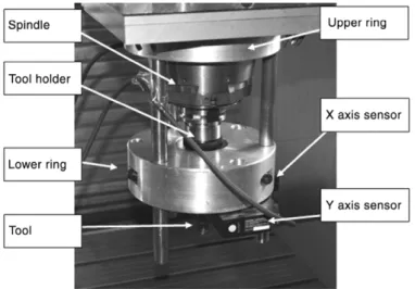
The tool dynamic behavior is investigated using a device were the tool body displacements are measured during the machining operation. TheFig. 1presents the used device that is composed of two parts: the upper ring clamped around the spindle nose and the lower ring which supports the displacement sensors and allows the measurement of the tool axis displacements along the

X and Y directions in the spindle referential. The two rings are

maintained by three high-stiffness bars. Non-contact displacement sensors were used by the mean of LKG Keyence laser based

on the triangulation principle. The observation of the laser spot reflection on the target gives the distance between the laser and the target. The bandwidth of the sensors was 50 kHz that enables high frequencies acquisition. For a 16000 rev/min revolution speed, this acquisition rate enables 180 points per revolution i.e. a tool angular resolution equal to two degrees. In addition, the high resolution of the sensors (0

.

05

µ

m) enables accurate displacements measurements of the tool end mill.

While the tool is machining the part, the tool axis displacements and the spindle encoder signal are monitored. The high accuracy of the sensors embedded in the presented device with a high frequency rate will be useful for the prediction of the generated surface. Moreover, the interest of displacements measurements instead of acceleration or velocity is that it does not need any signal integration. So, the steady state component of the tool behavior can be obtained.

Due to the optical technology of the sensor, no lubricant was used for machining operation.

An inserted tooth cutter was used for the tests. The cutting tests were conducted on a 3 axis DMG machining center with a 20 mm diameter tool with two inserts. The tool overhang was 120 mm (Fig. 2).

This machine allows a 18000 rev/min maximum spindle speed. The part was a 27 Mn Cr 5 steel, which hardness was 20 HRC.

4. Signal processing

The analysis of the recorded data is conducted according to the following steps:

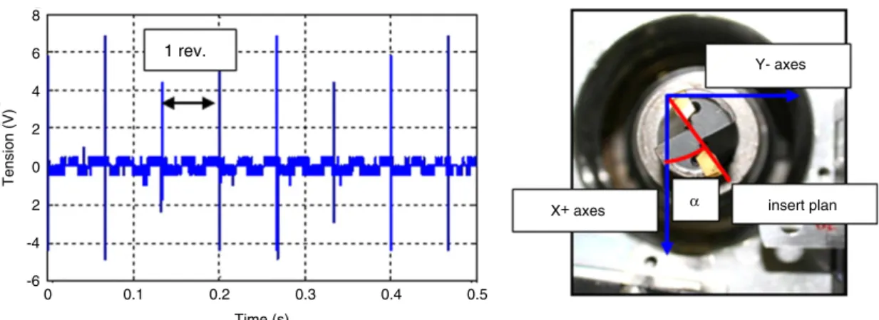
(1) Analysis of the spindle encoder signal.

The spindle encoder signal is a sampled signal which reaches its peak at a given spindle angular position as shown on

Fig. 3. This angular position corresponds to the ‘‘zero’’ reference angle. Therefore, the tool angular position for each sample point of the signal can be obtained.

Fig. 3. Spindle encoder signal (left). ‘‘Zero’’ reference angular position of the tool in the machine referential (right).

Fig. 4. Signal before (left) and after processing (right). The graph in the middle is a magnified display of 3 tool revolutions before signal processing (gray) and after processing

(black).

(2) Extraction of each tool revolution:

The spindle encoder signal is used in order to separate each tool revolution in the measurement displacement files. (3) Calculation of the average ‘‘off-machining’’ signal during one

revolution:

From each single tool revolution, the average one revolution off-machining signal is calculated. The off-machining signal period is selected before the tool entrance into the part. As a consequence, this average tool displacement includes the effects due to geometric (tool run out) and dynamic disturbances (unbalanced effects due to the tool rotation). (4) Subtraction of the averaged off-machining signal is applied to

the raw signal:

For a given step of time ti, the angular position

θ

i is calculated using the spindle encoder data. For this angular

position

θ

iat time ti, the average off-machining displacement

X

(θ

i

)

[resp. Y

(θ

i

)

] is subtracted to the X

(

ti

)

[resp. Y

(θ

i

)

] raw displacement. At each step of time, the subtraction is repeated for the corresponding angular position of the tool.

The four steps are processed by the software in time domain and start at the end of the operation.

The resulting signal (Fig. 4) leads to the effective tool deflection during the machining operation. The obtained signal should not contain any disturbance due to the tool shank geometric defaults.

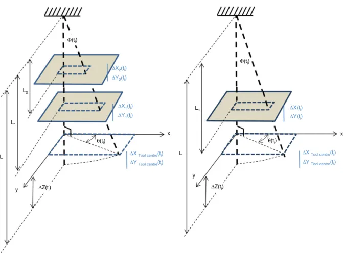
5. Surface topography computation

This part presents the different steps for the calculation of the cutting edges trajectories which is a preliminary step to compute

Fig. 5. Principle of the modeling: tool axis and one cutting edge trajectories with and without vibrations.

Fig. 6. Calculation of the tool effective deflection. With two distinct measuring planes (left) and one measuring plane (right).

the surface topography. The Fig. 6 simply illustrates the way the cutting edge positions are obtained. It is assumed that the tool trajectory followed by the machine axes is the same as the trajectory programmed on the machining center. So, the tool nominal trajectory is obtained from the spindle velocity and the feed speed ordered by the operator. Moreover, the trajectory is considered as a straight line in our case. Then, the tool vibrations are superimposed to the nominal tool trajectory (Fig. 5).

During preliminary investigations, tests with 4 non-displace-ment sensors in two different planes, the same tool and the similar cutting conditions were performed. With these tests the deflection mode of the tool could be calculated and the following conclusions were found:

•

The tool vibration mode can be compared to a clamped-free beam first vibration mode.

•

The height of the clamping plane of the tool in the tool holder is almost constant and is located near the tool holder level. Following these observations, the main hypothesis in the tool deflection calculation is that the tool deformation is assumed to be linear as show onFig. 6. As a result of the tool displacements obtained with the two laser sensors in one plane, the effective tool deflection at the cutting edges level can be extrapolated using this linear hypothesis.

The different steps for the flank edge trajectory prediction are given below and are illustrated inFig. 7.

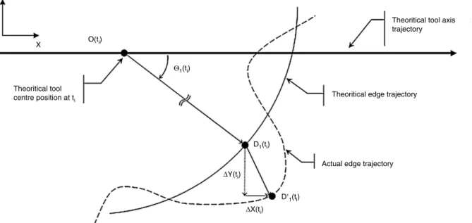
At a given time ti, the tool measured displacements are superimposed to the theoretical edge positions following Eq.(1):

−−−→ (OD′1)ti

  

Actual edge position

= −(−−OD→1)ti

  

Theoretical edge position

+ −→∆ti



Tool axis deflection

Fig. 7. Edge position calculation principle; D1(ti)and D′1(ti)are respectively the theoretical and actual edge 1 positions at time ti.∆X(ti)and∆Y(ti)are the measured tool

axis displacements in X and Y directions.

Fig. 8. Example of simulations: flank milling (left) and end milling (right).

Eq.(1)can be expanded as:

−

−−

→

(

OD′₁

)

ti

=



RD1

×

cos

(θ

1

(

ti

))

RD1

×

sin

(θ

1

(

ti

))



+



∆X

(

ti

)

∆Y

(

ti

)



(2) where

θ

1is the angular position of the edge 1.

For the points of the end-mill edges (located below the tool radius), the way their positions are calculated is slightly different: since a deflection angle is observed between the tool actual axis at time ti, the displacement value∆z(ti)is also taken into account. ∆z₍ti)

=

l

.(

1

−

cos

ϕ

(ti)

)

(3) where:

l is the length between the XY measurement plane and the tool

clamping plane.

ϕ

is the tool deflection angle calculated with∆x₍ti)and∆y(ti)using the Eq.(4): tan

ϕ

₍ti)

=



∆x2_(t i)

+

∆y 2 (ti) l

.

(4)

The positions are calculated for a meshing of points along the edge line and the calculation is repeated at each step of time of the simulation based on the angular step motion of the tool. At this stage, the cutting edge line positions in the spindle referential are known in three dimensions and for each step of time. In order to model the machined surface, the surface envelope swept by the cutting edges is then computed by storing the coordinates of the

Fig. 9. Machined (top) and calculated (bottom) surface in the case of a flank milling

operation with N=5000 tr/min, f =0.1 mm, axial depth of cut=2 mm, radial depth of cut=1 mm. Feed motion is along the X axis.

extreme points of the edges lines. Two types of calculated surfaces corresponding to flank milling and end milling are displayed on

Fig. 8.

6. Experimental validation

An experimental validation has been conducted in order to compare predicted and measured surface profiles. The machining tests were performed in flank and end milling with the parameters inTable 2.

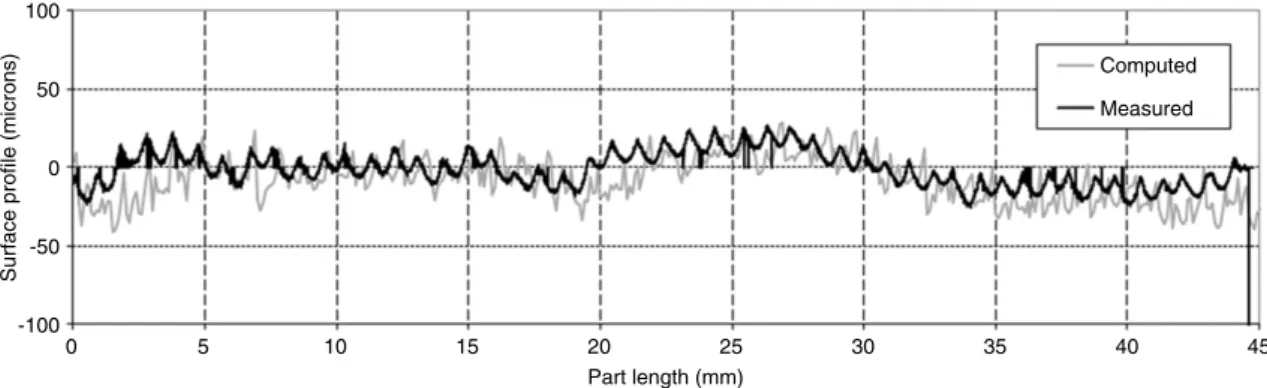
The machined and predicted surfaces for test no. 1 are displayed onFig. 9. TheFigs. 10–12show the surface profiles measured on the machined part (black profile) and computed with the proposed method (gray profile) for the 3 machining tests in flank and end milling. The equipment used was a Wyko optical profiling system. 3D surface maps of the samples were obtained.

The Figs. 10–12show a good correlation between the mea-sured and computed profiles in terms of shape and amplitude.

Fig. 10. Test 1 — Comparison between the computed and the measured profiles in flank milling with N=5000 tr/min, f =0.1 mm, axial depth of cut=2 mm, radial depth of cut=1 mm.

Fig. 11. Test 2 — Comparison between the computed and the measured profiles in flank milling with N=5000 tr/min, f =0.1 mm, axial depth of cut=2.5 mm, radial depth of cut=0.5 mm.

Fig. 12. Test 3 — Comparison between the computed and the measured profiles in end milling with N=11,000 tr/min, f=0.2 mm, axial depth of cut=0.15 mm, radial depth of cut=20 mm.

Table 2

Machining parameters of the 3 validation tests.

Spindle velocity (rpm) Feed-per-tooth (mm) Axial depth-of-cut (mm) Radial depth-of-cut (mm)

Test 1 — Flank milling 5,000 0.1 2 1

Test 2 — Flank milling 5,000 0.1 2.5 0.5

Test 3 — End milling 11,000 0.2 0.15 20

The roughness parameter Ra values obtained from measurement and from prediction are compared in the chart for the three tests inTable 3.

The predicted Ra values correlate better with measurements in flank milling than in end milling. That can be explained by the lower displacements values along the z-axis than in X and

Y directions obtained with the bending of the tool. This leads

obviously to a higher accuracy of the predicted edges trajectories along the X and Y axis than Z . In this study, the tool deflection was assumed to be linear and the clamping plane at a constant z level.

In order to improve the correlation in end milling, a more realistic model of the tool bending should be established.

7. Conclusions

This paper focuses on the dynamic behavior of a milling tool using tool center point methodology. The presented device allows the monitoring of the tool body displacements during the milling operation using two laser sensors. A geometrical model is presented where the actual edges positions are calculated at

Table 3

Measured and predicted Ra values for 3 machining operations.

Ra(µm) Ra(µm) Error (%) Measurement Prediction

Test 1 — Flank milling 5.01 5.62 12 Test 2 — Flank milling 6.76 6.09 11 Test 3 — End milling 1.15 0.93 23

each step of the simulation time taking account of the measured vibrations. The tool end mill is modeled as a clamped-free beam. The novelty of this study is that the deflection of the tool body is taken into account in the modeling and the height variations occurring at the tool end due to the deflection are calculated. This leads to the surface envelope swept by the edges along the tool path and the surface topography for peripheral and end milling. The surface predictions are compared with experimental tests and the results compare well.

Acknowledgments

This project has been supported by the CTDec (Technical Center for Machining of Small Part) and Arve Industry Consortium. Thanks are also addressed to Romain Brendlen for his technical support.

References

[1] Tlusty J, Polacek M. The stability of machine tools against self excited vibrations in machining. In: Proceedings of the ASME. Production engineering research conference. 1963.

[2] Tlusty J, Andrews GC. A critical review of sensors for unmanned machining. CIRP Annals — Manufacturing Technology 1983;32:563–72.

[3] Byrne G, Dornfeld D, Inasaki I, Ketteler G, König W, Teti R. Tool Condition Monitoring (TCM) — the status of research and industrial application. CIRP Annals — Manufacturing Technology 1995;44:541–67.

[4] Benardos PG, Vosniakos GC. Predicting surface roughness in machining: a review. International Journal of Machine Tools and Manufacture 2003;43: 833–44.

[5] Lou SJ, Chen JC. In-process surface recognition of a CNC milling machine using the fuzzy nets method. Computers & Industrial Engineering 1997;33: 401–4.

[6] Wang M, Chang H. Experimental study of surface roughness in slot end milling AL2014-T6. International Journal of Machine Tools and Manufacture 2004;44: 51–7.

[7] Montgomery D, Altintas Y. Mechanism of cutting force and surface generation in dynamic milling. Journal of Engineering for Industry 1991;113:160–8. [8] Altintas Y, Engin S. Generalized modeling of mechanics and dynamics

of milling cutters. CIRP Annals — Manufacturing Technology 2001;50: 25–30.

[9] Lee KY, Kang MC, Jeong YH, Lee DW, Kim JS. Simulation of surface roughness and profile in high-speed end milling. Journal of Materials Processing Technology 2001;113:410–5.

[10] Kline WA, Devor RE, Shareef IA. Prediction of surface accuracy in end milling. Journal of Manufacturing Science and Engineering, Transactions of the ASME 1982;104:272–8.

[11] Chang H, Kim J, Kim IH, Jang DY, Han DC. In-process surface roughness prediction using displacement signals from spindle motion. International Journal of Machine Tools and Manufacture 2007;47:1021–6.

[12] Omar OEEK, El-Wardany T, Ng E, Elbestawi MA. An improved cutting force and surface topography prediction model in end milling. International Journal of Machine Tools and Manufacture 2007;47:1263–75.

[13] Surmann T, Biermann D. The effect of tool vibrations on the flank surface created by peripheral milling. CIRP Annals — Manufacturing Technology 2008; 57:375–8.

[14] Arizmendi M, Campa FJ, Fernández J, López de Lacalle LN, Gil A, Bilbao E, et al. Model for surface topography prediction in peripheral milling considering tool vibration. CIRP Annals — Manufacturing Technology 2009;58:93–6. [15] Jiang H, Long X, Meng G. Study of the correlation between surface generation

and cutting vibrations in peripheral milling. Journal of Materials Processing Technology 2008;208:229–38.