Science Arts & Métiers (SAM)
is an open access repository that collects the work of Arts et Métiers Institute of
Technology researchers and makes it freely available over the web where possible.
This is an author-deposited version published in: https://sam.ensam.eu
Handle ID: .http://hdl.handle.net/10985/8586
To cite this version :
Moises SOLIS, Florent RAVELET, Sofiane KHELLADI, Farid BAKIR - Experimental and Numerical Analysis of the Flow Inside a Configuration Including an Axial Pump and a Tubular Exchanger - In: ASME 2010 3rd Joint US-European Fluids Engineering Summer Meeting
collocated with 8th International Conference on Nanochannels, Microchannels, and Minichannels, Canada, 2010 - Proceedings of the 3rd Joint US-European Fluids Engineering Summer Meeting and 8th International Conference on Nanochannels, Microchannels, and Minichannels - 2010
Any correspondence concerning this service should be sent to the repository Administrator : [email protected]
EXPERIMENTAL AND NUMERICAL ANALYSIS OF THE FLOW INSIDE A
CONFIGURATION INCLUDING AN AXIAL PUMP AND A TUBULAR
EXCHANGER
Mois´es Solis, Florent Ravelet,a)Sofiane Khelladi, and Farid Bakir
Arts et Metiers ParisTech, DynFluid, 151 boulevard de l’Hˆopital, 75013 Paris, France.
(Dated: Proceedings of 3rd Joint US-European Fluids Engineering Summer Meeting,) (August 1-5 2010, Montreal, Canada, FEDSM-ICNMM2010-30723)
In centrifugal and axial pumps, the flow is characterized by a turbulent and complex behavior and also by physical mechanisms such as cavitation and pressure fluctuations that are mainly due to the strong interactions between the fixed and mobile parts and the operating conditions. These fluctuations are more important at the tip clearance and propagate upstream and downstream of the rotor. The control of the fluctuating signal amplitudes can be achieved by incrementing the distance between the components mentioned above. This paper presents experimental and numerical results concerning the operation of a configuration that includes an axial pump and a bundle of tubes that mimics the cool source of a heat exchanger. The pump used in the tests has a low solidity and two blades designed in forced vortex, the tip clearance is approximately 3.87% of tip radius. The experimental measures were carried out using a test bench built for this purpose at the DynFluid Laboratory which was accomodated conveniently with a variety of instruments. Firstly, the characteristic curves were drawn for the pump at 1500 rpm and then a set of measurements concerning the use of pressure sensors was done in order to recover for different flow rates the static pressure signals upstream and downstream the pump and the exchanger. The pressure fluctuations and the performance curve were compared to the numerical results. The numerical simulations were carried out by using a Fluent code, the URANS (Unsteady Reynolds Averaged Navier-Stokes) approach and the k-ω SST turbulence model were applied to solve the unsteady, incompressible and turbulent flow. To record the fluctuating pressure signal, virtual sensors were necessary and placed at the same positions as in the experiments.
Keywords: Axial Pump, Pressure Fluctuations, Cavitation, Tubular Exchanger, Test Bench
NOMENCLATURE
Roman characters
c [mm] Chord length
F [Hz] frequency
H [m] Static head and static head at nominal point p [mm] 2πr/z, circumferential distance P [Pa] Pressure Q [m3/h] Flow rate r [mm] Radius s [-] p/c, Solidity Greek characters β [o] Blade angle δt [mm] Tip clearance η [-] Hydraulic efficiency ρ [kg.m−3] Density Subscripts 1 [-] Inlet BP [-] Blade passage ef f [-] Effective h [-] Blade hub
midspan [-] 50% of blade span
N [-] Nominal
R [-] Rotational
ref [-] Reference
t [-] Blade tip
a)Electronic mail: [email protected]
I. INTRODUCTION
The design of an efficient, quiet and reliable axial-flow pump is a challenge for the designers nowadays. The main difficulty is the existence of various geometrical pa-rameters that have a direct influence on the hydraulic performance. A solution to this problem is to analyze and better understand of the flow field inside the rotating and stationary parts with the help of numerical simulations and experimental tests. It is well known that an axial pump generates a complex flow field which is character-ized by the presence of physical mechanisms and pressure fluctuations. In this kind of pump configuration, the rel-ative motion between the rotating and stationary part causes strong interactions that are mainly associated to the blade passing frequency and are more important close to the tip clearance in the case of axial pumps and close to the tongue for centrifugal pumps. A potential reduc-tion of these interacreduc-tions can be achieved by varying the distance between the fixed and the mobile parts of the configuration.
Many research works have been done in the domain of axial pumps covering the cavitation, pressure fluctua-tions and design methods. The influence of the tip clear-ance was reported by Mitchell [1] who investigated ex-perimentally an axial pump. This work pointed out the existence of a critical tip clearance below which surface cavitation at the blade tip occurs first and above which
hal-00505772, version 1 - 3 Sep 2012
2 vortex cavitation due to the clearance flow occurs first.
Laborde et al. [2] found an optimum clearance geome-try to eliminate clearance cavitation through the study of cavitation patterns under different operations and ge-ometrical conditions. The influence of these cavitation patterns were determined by cavitation tests on an ax-ial flow pump by Horie et al. [3]. Over a wide range of operating conditions, a little change of pump head was observed when the cavitation on the blade surface was developed considerably. Others researchers analyzed the effects of guide vanes and rear stator. Kaya [4] experi-mentally studied two different axial flow pump impellers with and without guide vanes. Using guide vanes, the total pump efficiency was increased by about 3%. Gao et al. [5] investigated the effects of including a rear stator on flow fields using for his studies two water-jet pumps with and without a rear stator. They found a good agreement with the experimental results with improvement on the static pressure and the efficiency.
Not much work has been done to establish a relation-ship between cavitation development and the pressure fluctuations of an axial-flow pump. Saito [6] investigated the change in pressure fluctuations spectrum due to cav-itation and pointed out that it mainly depends on the tip clearance cavitation development. Fu-jun et al. [7] analyzed the flow in axial-flow pump through transient simulations and large eddy simulation (LES), obtaining the pressure fluctuations under various operation condi-tions. The maximum amplitude takes place at the inlet of impeller and they increases from hub to tip, but decreases at the middle area. The fluctuation becomes stronger as the flow rate is far from optimum operation point.
Another important factor of an axial pump is the blade design. Vad et al. [8] numerically compared two axial-flow pump rotors designed in free vortex and non-free vortex design having identical basic geometrical and flow rate parameters. He concluded that non-free vortex de-sign is an efficient method to increase the specific per-formance but as a drawback, the risk of cavitation also increases. On the other hand, for the non-free vortex ro-tor the efficiency drops more intensely with increase of tip clearance and the noise level may be lower than for the free vortex rotor. A similar work was done by Ida [9] with experiments on a forced-vortex impeller in an ax-ial flow fan without inlet vanes, assuming that the axax-ial velocity component is uniformly distributed from hub to tip.
Numerical calculations using CFD codes are an impor-tant tool to accurately predict the axial pump behavior. Miner [10] used a commercial code to compute the flow field within the first stage impeller of a two stage ax-ial flow pump, showing that the numerical results closely matched the shapes and magnitudes of the measured pro-files. Other examples are the works of DeSheng et al. [11] who simulated using Fluent code the flow field of a high efficiency axial-flow pump. He found that the static pres-sure on prespres-sure side of rotor blades increases slightly at radial direction, and remains almost constant in
circum-ferential direction at design conditions, while it increases gradually from inlet to exit on suction side along the flow direction. The experimental results showed that the inlet flow is almost axial and the prerotation is very small at design conditions.
Concerning the configuration formed by an axial pump and a tubular heat exchanger, the understanding of the flow behavior does not seem to be clear especially when the analysis is focused on the pressure fluctuations and the cavitation in the region upstream of the exchanger. The current paper presents an experimental and numeri-cal investigation of the interaction between an axial pump and a bundle of tubes that mimics the cool source of a heat exchanger. The experimental measurements were the static head rise, the pressure fluctuations upstream and downstream the rotor for different flow rates. The axial flow pump used for the experiments was a particu-lar rotor of low solidity, two blades and the tip clearance is about 3.87% of tip radius. On the other hand, numer-ical simulations were carried out using the URANS (Un-steady Reynolds Averaged Navier-Stokes) approach and the k-ω SST turbulence model were applied to solve the unsteady, incompressible and turbulent flow. In the un-steady calculations, virtual sensors were used to recover the fluctuating pressure signal at the same positions as in the experiments.
II. GEOMETRICAL CONFIGURATION AND OPERATING CONDITIONS
For this study, the configuration is based on an axial-flow pump and a bundle of tubes hereafter designated by the expression ”tubular exchanger” though no heat is actually exchanged in the reported works. It can be placed at several distances downstream of the pump (see figure 1) in order to study the influence of this distance on the level of pressure fluctuations. In this Paper, results for only one position are reported.
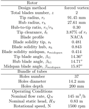
The test loop was conditioned with some instruments positioned conveniently to measure the static pressure, flow rate, electric power and pressure fluctuations. The rotor used has a particular geometry and low solidity. It has two blades designed in forced vortex and presents an important tip clearance. The main geometrical charac-teristics of the reference pump and flow parameters are summarized in table 1.
III. COMPUTATIONAL DOMAIN AND NUMERICAL PROCEDURE
In order to compare the numerical and experimental results, the domain for the calculations was obtained from the original geometries of the test bench used during the experimental measurements. The calculation domain extends from the suction and discharge pipe (see figure 2). To avoid any influence of boundary limits, they were
Rotor
Design method forced vortex Total blades number, z 2
Tip radius, rt 91.45 mm
Hub radius, rh 27.61 mm
Hub-to-tip ratio, rt/rh 0.30
Tip clearance, δt 3.87% of rt
Blade profile NACA
Blade solidity tip, st 0.481
Blade solidity hub, sh 0.843
Blade solidity midspan, smidspan 0.414
Tip blade angle, βt1 14.36o
Hub blade angle, βh1 14.71o
Midspan blade angle, βmidspan 15.87o
Bundle of tubes
Holes number 37
Holes diameter 14.2 mm
Holes depth 200 mm
Operating Conditions
Nominal flow rate, QN 145 m3/h
Nominal static head, HN 0.83 m
Rotational speed, N 1500 rpm
TABLE I. Rotor and ”tubular exchanger” geometrical char-acteristics and operating conditions
FIG. 1. Geometry of the configuration including an axial pump and exchanger
FIG. 2. Computational domain
appropriately extended to let the flow develop, ensuring numerical stability and minimizing boundary conditions effects. On the other hand, it is clear that the pres-ence of complex geometries such as the rotor and the aspiration components will make the mesh hybrid. So, the entire domain was divided into various sub-domains. Thus, the regions considered are the suction pipe, rotor, tip clearance, tubular exchanger and discharge pipe. For the parts before the rotor and after the exchanger, the mesh types is a mixture of tetrahedral and hexahedral elements. Concerning the fluid volume of the rotor, the mesh was refined around the blades and the elements were tetrahedral. In the case of the tip clearance which has the shape of a ring, the elements considered were hexahedral following the flow direction, with 20 cells in the radial direction. The exchanger region is modeled by equidistant hexahedral cells distributed in the z direc-tion. A mesh independency study was not made because of the significant number of components, but the retained mesh size was considered sufficient and its distribution adequate to validate the final results. The flow mod-eling was achieved by Fluent code based on the finites volumes method. The equations governing the fluid such as the continuity, momentum and turbulence equations were solved for the steady calculations in the moving ref-erence frame and the sliding mesh technique was applied for the unsteady calculations, allowing to simulate the three-dimensional flow inside the pump and the interac-tions between the rotor and the external casing. The turbulence effects was simulated by using the k-ω SST model and the boundary limits imposed are an uniform normal velocity at inlet and the outflow condition at the outlet domain. The time dependent term scheme was a second order implicit. The pressure-velocity coupling is performed using the SIMPLE algorithm ”Semi-Implicit Method for Pressure Linked equations”. Second order, upwind discretization is used for convection terms and central difference schemes for diffusion terms. The time step for the unsteady calculations has been set to 1.104 s that will allow to have a good resolution in time and a good frequency resolution. Please note that it is also the experimental data acquisition rate. The simulations are carried out by doing a steady simulation to construct the performances curves and using then the output as an initial condition for the unsteady simulations. To inves-tigate local boundary layer variables, the mesh used in the rotor is not the most adequate given the complexity of the geometry, but the global ones are well calculated. Thus, approximately 2.5 million cells were used for the steady and unsteady calculations which will be validated by the experimental results. The table 2 summarizes the cells number employed for each region of the complete configuration considered for the modeling and the figure 3 shows some details of the grid on the rotor and the exchanger. On the other hand, a relatively large amount of time steps are required to pass the transient and to achieve a stable periodic solution. Virtual sensors were placed in the same positions as they were on the test
4
FIG. 3. Meshes of the rotor and exchanger domain
facility to record time series of the static pressure. The data are analysed in the frequency domain using the Fast Fourier Transform.
Domain Cells number Suction pipe 425 621 Rotor 1 560 793 Tip Clearance 208 860 Exchanger 45 954 Discharge pipe 331 292 Total 2 572 520
TABLE II. Total cells number for the configuration axial pump and exchanger
IV. EXPERIMENTAL FACILITY
The experimental tests were carried out at the Dyn-Fluid laboratory. For this purpose, an experimental test
FIG. 4. Scheme of the DynFluid axial pump test-ring
FIG. 5. Pressure sensor positions in the test facility
facility was designed and adapted to the existing installa-tion which is composed of two independent but intercon-nected loops: one for centrifugal pumps and another for axial pumps. The test bench is shown in figure 4. The axial-flow pump loop used for this investigation consists of:
• Two storage tanks with a capacity of 4 m3that can
be filled and emptied using two electrical butterfly control valves that are also used to adjust the flow rate accurately.
• A liquid ring vacuum pump that controls the pres-sure at the free surface inside the two storage tanks. • An electromagnetic KROHNE flowmeter placed downstream of the axial pump (accuracy ± 0.5 m3/h).
• A 22 kW alternative motor powered by a frequency inverter to drive the tested axial pump at different rotational speeds (accuracy ±0.05 kW).
• A magnetic tachometer to measure the rotational speed (accuracy 0.1%).
• A transparent acrylic cover in the zone of the axial pump to observe the flow and others aspects like the cavitation development.
• A centrifugal pump to drive the fluid toward the ax-ial pump when it is necessary. It is situated about
50 pipe diameter upstream of the axial pump, and is mounted between two DilatoFlex elements in or-der to attenuate the propagation of pressure fluc-tuations.
• Metallic differential manometers backed up by piezoresistive pressure sensor (accuracy ±3 mBars). • A temperature probe (accuracy 1%): the average
temperature during the tests was 18o.
• Four pressure sensor PCB Piezotronics (Model 106B51) that are flush-mounted and placed at var-ious positions upstream and downstream of the ro-tor (see details in figure 5).
i) Sensor c1 positioned approximately at a distance 119.6 cm from the rotor (leading edge).
ii) Sensor c2 positioned approximately at a distance 14.4 cm from the rotor (leading edge).
iii) Sensor c3 positioned approximately at a distance 54.4 cm from the rotor (leading edge).
iv) Sensor c4 positioned approximately at a distance 88.9 cm from the rotor (leading edge).
V. EXPERIMENTAL AND NUMERICAL RESULTS GLOBAL PERFORMANCES CURVES
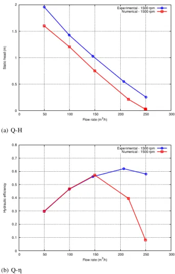
The first series of measurements concern the overall performances at 1500 rpm for the configuration without the tubular exchanger. For this purpose, experimental and numerical tests were carried out to determine the operating point. The static pressure measurements were made at a distance upstream of the rotor (leading edge) of 132.1 cm and a distance downstream of the rotor (lead-ing edge) of 116.9 cm. Figure 6 presents the global sta-tionary pump performances compared to the experimen-tal measurements. For the Q H curve the trend is the same for the numerical and experimental results, but the experimental curve is approximately 0.2 m higher than the numerical curve. Concerning the hydraulic efficiency, there is a very good agreement for flow rates below 150 m3/h. Above this flow rate, there is a strong discrepancy
which will have an influence on the determination of the nominal point. Thus, the numerical nominal point does not match with the experimental one. The numerical point is 145 m3/h and 0.83 m and the experimental one
is 210 m3/h and 0.54 m. The differences can be explained
by the lack of precision on the electric power measure-ment and differential pressure. Other reason of the static pressure difference would be that the rotor geometry is particular and differs from that obtained by the man-ufacturing process. Please also note the very peculiar geometry of the pump, with low solidity and high stag-ger angle. Visualisation using cavitation have confirmed that the flow is adapted at a flow rate of 210 m3/h in the experiment.
FIG. 6. Comparison between the numerical and experimental results of characteristics curves
VI. PRESSURE FLUCTUATIONS
A series of measurements was performed for the con-figuration with axial pump and the other including the pump and the tubular exchanger. Concerning the sin-gle pump, three flow rates (50 m3/h, 100 m3/h and 145
m3/h) were tested and information about pressure signals
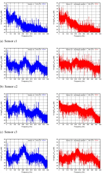
were recorded and compared. In the tests, four pressure sensors (c1, c2, c3 and c4) were distributed upstream and downstream of the rotor (see figure 5 for details). The figure 7 shows the comparison of frequency spectra ob-tained from the four sensors at different flow rates. The first impression of the results reveals that the spectra are different between the pressure sensors. There is a small peak at FR= 25 Hz that could be linked to a small
un-balance in the system. The main peak is at the blade passing frequency FBP = 50 Hz and the analysis is
fo-cused on this peak. Its amplitude is high at inlet pump (sensor c1), but it decreases as we move away from the pump (sensor c4) at any flow rate. The apparition of peaks at frequencies lower than FBP is due to the
cen-trifugal pump which was used to ensure the flow rate to
6
FIG. 7. Comparison of pressure frequency spectrum for the single pump. Pref = 1Pa
the axial pump. On the other hand, it can be seen that for the four sensors c1, c2, c3 and c4 the fluctuations in-crease when the flow rate begins to rise from 100 m3/h to 145 m3/h.
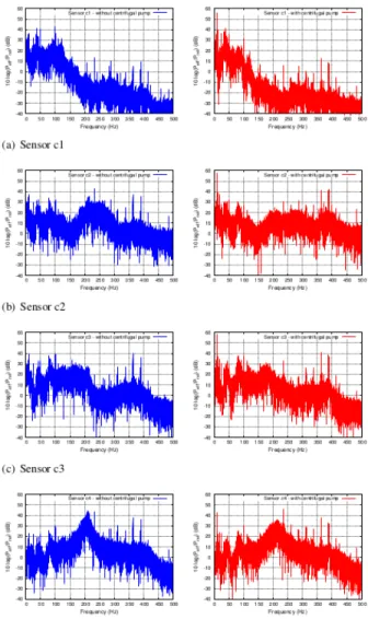
The influence of inlet conditions were studied for the configuration single pump in order to determine the im-portance of pressure inlet. So, some measurements of pressure for a flow rate of 92 m3/h were made and
com-pared when the axial pump works with the centrifugal pump and when it works alone. In this case, the flow rate mentioned was the maximum we could obtain from the circuit with the axial pump operating. The inlet pressure without centrifugal pump was approximately -105 mBar and with centrifugal pump it was -30 mBar. From the figure 8, which was obtained by a FFT analysis, we can point out specially at FBP some differences in relation
to pressure amplitudes. In most of sensors except sensor c2, the amplitudes are lower when the centrifugal pump
FIG. 8. Comparison of pressure frequency spectrum for the single pump at 92 m3/h with different suction conditions. Pref = 1 Pa
is operating in this way varying the suction pressure and the turbulence intensity. Thus, the importance of in-let conditions is manifested by the pressure fluctuations results that could be considered when performing experi-mental tests and secondly a solution to decrease pressure fluctuations instead of having to do modifications to the geometry.
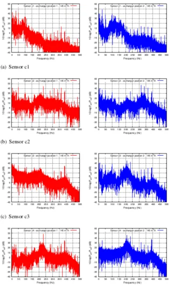
In order to establish a relation between pressure fluctu-ations and the position of the exchanger. Two positions were tested, position 1 which corresponds when the ex-changer is near to the pump (exex-changer between sensor c2 and c3) and position 2 when the exchanger is far from the pump (exchanger between sensor c3 and c4). The ex-changer was fixed adequately to prevent movement dur-ing operation of the circuit. The flow rates tested were two (145 m3/h and 210 m3/h). First, considering a flow rate of 145 m3/h (see figure 9), the spectra indicate a re-duction of amplitudes in sensor c1 placed upstream the
FIG. 9. Comparison of pressure frequency spectrum for con-figuration including axial pump and exchanger at 145 m3/h. Pref = 1 Pa
axial pump and also for c2 located downstream the pump but before the exchanger. Taking into account the sen-sor before and after the exchanger, we can perceive that the exchanger plays the role of an attenuator reducing the pressure amplitudes (see for example sensor c3 for position 1 and c4 for position 2). Comparing sensor c4, it can be noted that the amplitudes showed reveals the differences because in position 1 of exchanger, c4 is far of the exchanger discharge and in position 2 of exchanger it is located just off the exchanger.
At 210 m3/h, the results in figure 10 show that the fluctuations are reduced for sensor c1 placed before the pump, however the sensors downstream the pump have different behaviors depending of the exchanger position. For example, the fact of moving away the exchanger does not improve the fluctuations rather they worse in sensor c2. The differences in spectra of sensor c3 are due be-cause in position 1, it is just after the exchanger and in
FIG. 10. Comparison of pressure frequency spectrum for con-figuration including axial pump and exchanger at 210 m3/h. Pref = 1 Pa
position 2, it is before. But in sensor c4, the differences are due to the proximity concerning the exchanger out-let. The amplitudes in position 1 are lower than position 2 because, the fluctuations had more time to dissipate.
Concerning the influence on pressure fluctuations of the configuration including or not the exchanger has been made. In the figure 11, we can see the influence of the exchanger in the pressure field measured by four sensors at 145 m3/h. For sensor c1 and c2, it is clear the influence
of the exchanger disturbs and increase the fluctuations being lower when the exchanger is not considered. In relation to the sensors c3 and c4, the amplitudes are lower than those when the pump works alone due mainly to the exchanger which plays the role a attenuator.
It can be seen that the spectral analysis shows vari-ous peaks at several frequencies related to the rotating frequency and also to blades number and their harmon-ics. To model the pressure fluctuations, unsteady cal-culations were necessary. The convergence of these type
8
FIG. 11. Comparison of pressure frequency spectrum for configuration single pump and including axial pump and ex-changer at 145 m3/h. P
ref = 1 Pa
FIG. 12. Numerical and Experimental comparison of the con-figuration including an axial pump and an exchanger
of calculations is achieved approximately in various rotor revolutions to obtain a periodic unsteady solution spe-cially of the static pressure and also other revolutions to get enough data to have a good frequency resolution con-cerning the frequency analysis. In this way, the instan-taneous static pressure was recorded by virtual sensors placed at the same positions as the test bench. Then the
pressure signals were analyzed and processed using the Fast Fourier Transform (FFT) with a Hanning Window as they were in the experimental measurements. The lack of time to let the simulations converge specially for the sensors placed downstream the rotor was an inconvenient to show all the numerical results in order to compare to experimental ones. So in this way, the recorded values of sensor c1 were confronted with the experimental values. The figure 12 illustrate the comparison between numer-ical and experimental signals, showing the differences at FBP of 8 decibels.
VII. CONCLUSIONS
Numerical and experimental tests were carried out at DynFluid Laboratory. For this purpose a test bench was built and coupled to the centrifugal pump loop. It was ac-commodated with several instruments to measure static pressure, electric power and pressure fluctuations. The study concerned a configuration including an axial pump and a bundle of tubes. Four sensors were distributed upstream and downstream the pump. In the numeri-cal simulations, virtual sensors collected the fluctuating pressure signal in the same positions as the experimental ones. The following conclusions can be retained:
i) The experimental nominal point (210 m3/h) does not
match with the numerical one (145 m3/h).
ii) The highest fluctuations occur upstream the rotor and increase with the presence of the exchanger. iii) Placing the exchanger after the rotor allows to
de-crease pressure fluctuations at outlet, but inde-crease those at inlet.
iv) The use of the centrifugal pump to ensure the flow rate to the axial pump modifies the inlet conditions. So, in this way a pressure fluctuations reduction will be detected when the axial pump is fed by the cen-trifugal one. Further numerical investigations with inlet boundary conditions that mimics this effect would be of great interest.
REFERENCES
[1] Mitchell, A. B., 1961. ”An experimental investiga-tion of cavitainvestiga-tion incepinvestiga-tion in the rotor blade tip region of an axial flow pump”. PhD thesis, Aeronautical Research Council.
[2] Laborde, R., Chantrel, P., and Mory, M., 1997. ”Tip clearance and tip vortex cavitation in an axial flow pump”. Journal Fluids Engineering, 119, pp. 680685.
[3] Horie, C., and Kawaguchi, K., 1959. ”Cavitation tests on an axial flow pump”. The Japan Society of Me-chanical Engineers, 2(5), pp. 187195.
[4] Kaya, D., 2003. ”Experimental study on regain-ing the tangential velocity energy of axial flow pump”. Energy Conversion & Management, 44, pp. 18171829.
[5] Gao, H., Lin, W., and Du, Z., 2008. ”Numerical flow and performance analysis of a water-jet axial flow pump”. Ocean Engineering, 35, pp. 16041614.
[6] Saito, S. ”The relationship between cavitation de-velopment and the velocity and pressure fluctuations of an axial-flow pump”. The Japan Society of Mechanical Engineers, 86-1485A, pp. 36823690.
[7] Fu-jun, W., Ling, Z., and Zhi-min, Z., 2007. ”Anal-ysis on pressure fluctuation of unsteady flow in axial-flow pump”. Journal of Hydraulic Engineering, 8, pp. 10031009.
[8] Vad, J., Bencze, F., Benigni, H., Glas, W., and Jaberg, H., 2002. ”Comparative investigation on axial flow pump rotors of free vortex and non-free vortex de-sign”. Periodica Polytechnica, Ser. Mech. Eng., 46, pp. 107116.
[9] Ida, T., 1970. ”Characteristics and flow condi-tions of a forced-vortex impeller of an axial flow fan:”. The Japan Society of Mechanical Engineers, 13(60), pp. 773780.
[10] Miner, S. M., 1997. ”3-d viscous flow analysis of an axial flow pump impeller”. International Journal of Rotating Machinery, 3(3), pp. 153161.
[11] De-Sheng, Z., Wei-Dong, S., Bin, C., and Xing-Fan, G., 2009. ”Numerical simulation and flow field measurement of high efficiency axial-flow pump”. Pro-ceedings of the ASME 2009 Fluids Engineering Division Summer Meeting August 2-6, 2009, Vail, Colorado, USA, pp. 18.