HAL Id: hal-01095749
https://hal.inria.fr/hal-01095749
Submitted on 16 Dec 2014
HAL is a multi-disciplinary open access
archive for the deposit and dissemination of
sci-entific research documents, whether they are
pub-lished or not. The documents may come from
teaching and research institutions in France or
abroad, or from public or private research centers.
L’archive ouverte pluridisciplinaire HAL, est
destinée au dépôt et à la diffusion de documents
scientifiques de niveau recherche, publiés ou non,
émanant des établissements d’enseignement et de
recherche français ou étrangers, des laboratoires
publics ou privés.
Survey of Deployment Algorithms in Wireless Sensor
Networks: Coverage and Connectivity Issues and
Challenges
Ines Khoufi, Pascale Minet, Anis Laouiti, Saoucene Mahfoudh
To cite this version:
Ines Khoufi, Pascale Minet, Anis Laouiti, Saoucene Mahfoudh. Survey of Deployment Algorithms in
Wireless Sensor Networks: Coverage and Connectivity Issues and Challenges. International journal of
autonomous and adaptive communications systems, Inderscience Publishers, 2017, 10 (4), pp.341-390.
�10.1504/IJAACS.2017.10009671�. �hal-01095749�
Survey of Deployment Algorithms in Wireless Sensor
Networks: Coverage and Connectivity Issues and
Challenges
Ines Khoufi
INRIA, Rocquencourt,
78153 Le Chesnay Cedex, France, Email: [email protected]
Pascale Minet
INRIA, Rocquencourt,
78153 Le Chesnay Cedex, France, [email protected]
Anis Laouiti
TELECOM SudParis, CNRS Samovar UMR 5157, 91011 Evry Cedex, France,
Email: [email protected]
Saoucene Mahfoudh
INRIA, Rocquencourt,
78153 Le Chesnay Cedex, France, [email protected]
Abstract: Wireless Sensor Networks (WSNs) have many fields of application, including industrial, environmental, military, health and home domains. Monitoring a given zone is one of the main goals of this technology. This consists in deploying sensor nodes in order to detect any event occurring in the zone of interest considered and report this event to the sink. The monitoring task can vary depending on the application domain concerned. In the industrial domain, the fast and easy deployment of wireless sensor nodes allows a better monitoring of the area of interest in temporary worksites. This deployment must be able to cope with obstacles and be energy efficient in order to maximize the network lifetime. If the deployment is made after a disaster, it will operate in an unfriendly environment that is discovered dynamically. We present a survey that focuses on two major issues in WSNs: coverage and connectivity. We motivate our study by giving different use cases corresponding to different coverage, connectivity, latency and robustness requirements of the applications considered. We present a general and detailed analysis of deployment problems, while highlighting the impacting factors, the common assumptions and models adopted in the literature, as well as performance criteria for evaluation purposes. Different deployment algorithms for area, barrier, and points of interest are studied and classified according to their characteristics and properties. Several recapitulative tables illustrate and summarize our study. The designer in charge of setting up such a network will find some useful recommendations, as well as some pitfalls to avoid. Before concluding, we look at current trends and discuss some open issues.
Keywords: area coverage, barrier coverage, coverage, deployment algorithms, full connectivity, grid, intermittent connectivity, node activity scheduling, point of interest coverage, sensor deployment, virtual forces, wireless sensors, WSN
Biographical notes: Ines Khoufi received her Computer Science Engineering and Master degrees from the National College of Computer Science (ENSI) in 2010 and 2011 respectively. Currently, she is a Ph.D. student in HIPERCOM2 research team at Inria. Her current research interest is on wireless sensor networks deployment and progressive discovery of an unfriendly environment.
Pascale MINET works at the Inria research center of Rocquencourt, near Versailles. She is head of the HIPERCOM (High Performance Communication) team. She got her qualification in advising PhD students in 1998 from the University of Versailles. Previously she got her PhD diploma in Computer Science, the University of Toulouse and her Engineer diploma in Computer Science in 1980 from
2
ENSEEIHT (Engineering school of Toulouse). Her research topics relate to wireless sensor networks and mobile ad hoc networks and more particularly energy efficiency, routing, node activity scheduling, multichannel communication, redeployment and quality of service in these networks. She is co-author of the OLSR routing protocol standardized at IETF.
Anis Laouiti is an associate professor at Telecom SudParis since 2006. Before, he did his Phd research work and worked as a research engineer within Hipercom team at Inria-Rocquencourt where he participated to the OLSR routing protocol design (RFC3626). His research covers different aspects in wireless ad hoc and mesh networks including protocol design, performance evaluation and implementation testbed.
Saoucene MAHFOUDH received her Computer Science Engineering degree from ENSI in 2005 and her Master degree from the University of Paris 6 in 2006. She obtained her Ph D diploma in 2010 from the University of Paris 6. Her research topics deal with energy efficiency, cross-layering, routing and redeployment in wireless sensor networks. After a post-doctoral fellow at Inria, she has been working at King AbdelAziz University since 2013.
1 Introduction
With the emergence of the Internet of Things (IoT), several billion electronic devices and machines will be able to be connected to one another via the Internet. The devices will be able to communicate without the intervention of humans. Such communication is called Machine-to-Machine communication, denoted M2M, and mobile wireless technology is an ideal technology to support M2M communication. These emerging technologies based on wireless communication can be autonomous and cope with changes without any human help. As an example, the fast and easy deployment of mobile wireless sensors in a temporary worksite is very useful for maintenance purposes and quality insurance. As these wireless sensor nodes are battery equipped, the deployment should be energy efficient in order to maximize network lifetime. Sensors can also be used for damage assessment after a disaster, when the network infrastructure has been damaged. In this case, the Wireless Sensor Network (WSN) operates in an unfriendly environment that can only be discovered progressively. However, some major challenges need to be tackled, such as:
• How to deal with the large volume of data produced. Collecting and exploiting these large data flows is commonly known as big data transfer and processing.
• How to organize communication. Communicating objects will exist everywhere. They are generally used to monitor a phenomenon. This phenomenon can be monitored by a single object (e.g. the temperature of coffee in a mug) or require collaboration between several objects, which are usually deployed in a predefined area. In the latter case, these objects need to communicate and organize themselves in the form of a network. That is the focus of this paper.
Depending on the size of the entity (area, barrier or point of interest) monitored, a multi-hop network may need to be deployed to enable the monitoring of this area as well as the delivery of the collected data. To meet the application requirements, the deployment of these communicating objects (e.g. sensor nodes) must ensure coverage and connectivity properties. Roughly speaking, coverage refers to the ability to detect events occurring in the entity monitored (e.g. area, barrier, point of interest) whereas connectivity refers to the ability to report this event to the sink.
1.1 Motivation
There are several types of coverage and connectivity problems in WSNs.
With regard to the coverage of the entity monitored we distinguish between area, barrier and point of interest coverage. Furthermore, the coverage can be full (i.e. any point of the entity is covered) or partial, depending on the application requirements. If the coverage is full, any point can be monitored by a single sensor node (i.e. simple coverage) or by several sensor nodes (i.e. multiple coverage), depending on the degree of robustness required. If the application requires short delays to detect an event, any point must be permanently covered. In other cases, any point is temporarily covered.
With regard to connectivity, if the application requires short delays to report the event detected to the sink, permanent connectivity is needed. Otherwise, intermittent connectivity is sufficient. An example is given by a mobile robot collecting data from disconnected islands of sensor nodes and, more generally, delay tolerant networks taking advantage of the mobility of data mules such as robots or people, etc.. If the application requires a high degree of robustness, multiple paths toward the sink are needed. Otherwise, a single path is sufficient.
As concerns the quality of data gathered, the application specifies its requirements for the time and space consistency of the data gathered. If both are required, a regular and uniform deployment is needed.
3 Usually, an initial deployment is provided. It can be
random (e.g. sensor nodes are dropped from a helicopter), all sensor nodes can be grouped together at an entry point, or they can form disconnected groups, each group consisting of a set of connected sensor nodes, etc. However, such a deployment usually fails to ensure the coverage and connectivity properties required by the application. For instance, some regions can be highly covered whereas others are poorly covered and may contain some coverage holes that are not monitored. Similarly, disconnected groups of sensors may fail to report the event detected to the sink. In both cases, the quality of data gathered is inappropriate, making, new a deployment necessary.
To save energy and maximize network lifetime, it is necessary after the final deployment to schedule node activity to make nodes sleep (e.g. redundant nodes for full coverage, useless nodes for partial coverage) while meeting the application requirements. Notice that node activity scheduling differs from sensor node deployment, because existing sensor nodes are only switched on or off but are not moved. This paper is organized as follows. This section ends with a description of representative use cases and the positioning of our contribution with regard to other surveys. Section 2 defines the coverage and connectivity issues encountered in wireless sensor networks, (WSNs). Section 3 deals with analysis criteria for deployment algorithms, and more particularly presents factors impacting the deployment, common assumptions and models adopted, as well as performance evaluation criteria. In Sections 4, 5 and 6, we focus on deployment algorithms ensuring coverage of area, barrier and point of interest respectively. Section 7, explores some energy-efficient optimization of a deployment, based on node activity scheduling. In Section 8, we provide guidelines to help the designer to select the deployment algorithm suitable for the application requirements. Finally, we discuss some trends and open issues for deployment algorithms in Section 9 before concluding in Section 10.
1.2 Representative use cases
Depending on the application requirements, we can distinguish the following use cases (UC) dealing with coverage and connectivity, and representative of most applications: UC1 monitoring of a temporary industrial worksite requires
full area coverage, permanent network connectivity and a uniform deployment of sensor nodes to reduce data gathering delays and provide a better balancing of node energy.
UC2 forest fire detection requires full area coverage in dry seasons and only 80% in rainy seasons. Permanent connectivity is required in both cases to alert the firefighters.
UC3 detecting and tracking of intruders in restricted areas. Such applications require full area coverage; furthermore, the most critical zones should be covered by more than one sensor node (i.e. multiple coverage). Permanent connectivity is also required.
UC4 monitoring of endangered wild species at some water points: the idea is to compute statistics about the number of individuals of this species from the number of individuals visiting the water point. A full or partial belt of sensor nodes is built along the water point depending on its size. Intermittent connectivity is usually sufficient. UC5 detection of intruders crossing a barrier (e.g. the border of a country, a door or windows in an apartment). Such applications require a barrier coverage with a permanent connectivity. Depending on the application requirements, one or several barriers are needed, the latter case being called multiple barrier coverage.
UC6 air pollution monitoring in a smart city. Partial area coverage is sufficient and intermittent connectivity can be compliant with the application requirements. UC7 instantaneous snapshot of measures taken at locations
predefined by the application. In precision agriculture, the goal is to detect the appearance of diseases in the crops. In a smart city, the goal is to track an air pollutant. Such applications require the coverage of static points of interest. Permanent connectivity may be not needed. Intermittent connectivity can be provided by mobile robots (e.g. tractors for precision agriculture).
UC8 tracking of wild animals or a truck fleet with embedded sensors. In such a case, different technologies can be used to track these mobile points of interest (e.g. Argos beacons for animals, 3G/4G systems for trucks). Depending on the application requirements, connectivity may be intermittent (e.g. animals) or permanent (e.g a truck fleet).
UC9 health monitoring of isolated workers, disabled people or elderly. They are considered as mobile Points of interest that must be permanently covered. Permanent connectivity is required.
All these uses cases will enable us to classify the coverage and connectivity problems encountered in the literature (see Table 1), according to the criteria defined more precisely in Section 2.
With the emergence of smart cities, different use cases can coexist simultaneously. For instance, air pollution monitoring, surveillance of parking lots, public lighting control, and pollutant tracking are examples of sensor deployments that will be very common in our cities in the near future.
1.3 Related work
In this section, we position our work with regard to other existing surveys and highlight our contribution. Existing surveys (2; 3; 4; 5; 6; 7; 8) introduce basic concepts related to coverage and connectivity. For instance, (2) focuses on how to ensure area coverage and how to deploy sensor nodes. (3) classifies coverage problems as coverage based on exposure and coverage exploiting mobility. Area coverage, point coverage and barrier coverage is another classification proposed and detailed in (4) and (5).
4
Area coverage Barrier coverage PoI coverage Full Partial Full Partial Static Mobile Simple Multiple Simple Multiple
Connectivity
Permanent Simple or multiple UC1 UC3 UC2 UC5 UC4 UC8 UC9
Intermittent UC6 UC4 UC4 UC7 UC8
Table 1 Classification of use cases.
In (6), the authors distinguish two coverage problems: static coverage and dynamic coverage. They also propose a study of sleep scheduling mechanisms to reduce energy consumption and analyze the relationship between coverage and connectivity. An overview of existing centralized and distributed deployment algorithms is given in (7). The authors in (8) discuss the different deployment algorithm strategies such as forces, computational geometry and pattern based deployment. These surveys are good references to have an overall view of coverage and connectivity issues in WSNs.
In this survey, we define the coverage and connectivity problems separately to provide a better understanding. The originality of our approach lies in a different viewing angle. We provide comprehensive definitions of coverage and connectivity with their possible variants. Indeed, these variants depend on the latency and robustness requirements that differ in the applications considered, leading to representative use cases. For each use case, we list some deployment algorithms found in the literature. We give a global analysis of the deployment problem by discussing the impacting factors, detailing the common assumptions and models adopted in the literature. Moreover, we propose some performance criteria to evaluate deployment algorithms. In order to help the designer to choose the most suitable deployment algorithms, we dedicate an entire section to questions and recommendations regarding coverage and connectivity problems. We also provide a section summarizing current trends and discuss open issues for deployment algorithms.
2 Coverage and connectivity problems in WSNs
2.1 Coverage
An area is said to be covered if and only if each location of this area is within the sensing range of at least one active sensor node.
In our work, we distinguish three types of coverage problems : Area coverage, Point coverage and Barrier coverage.
2.1.1 Area coverage
In the area coverage problem, the goal is to cover the whole area. Depending on the application requirements, full or partial coverage is required. However, if the number of sensors is not sufficient, full coverage cannot be achieved and the goal becomes maximizing the coverage rate.
• Full coverage
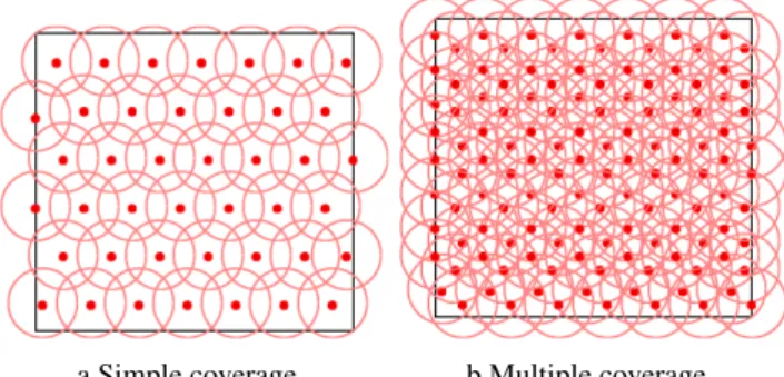
Applications such as battlefield monitoring require full area coverage. In these applications, every location is covered by at least one sensor node (1-coverage) or by k > 1 sensor nodes (k-coverage). Deploying sensors over a large area while ensuring full coverage and network connectivity may be expensive. However, full coverage with connectivity provides the best surveillance quality. In the following we detail one-coverage defined as simple one-coverage and k-one-coverage defined as multiple coverage, depending on the degree of robustness required by the application.
− Simple coverage
In WSNs, it is necessary to ensure full coverage of the area considered while deploying the minimum number of sensor nodes. This can be satisfied by covering every location in the field using at least one sensor node. Then information detected in this location should be reported to the sink. Many studies aim to minimize the number of nodes deployed while ensuring coverage and connectivity. For instance, the triangular lattice deployment provides full coverage, connectivity and uniform deployment using the minimum number of sensor nodes.
− Multiple coverage
Multiple coverage is defined as an extension of simple coverage and is denoted by k-coverage. It is specific to applications such as distributed detection, mobility tracking, monitoring in high security areas and military intelligence in a battlefield. Since the failure of a single node may result in the loss or corruption of important data, one degree of coverage is not sufficient for these applications. Such applications require highly accurate information in order to provide fault tolerance and allow good decisions to be made. The k-coverage deployment is defined as a sensor deployment pattern where each point in the area is covered by at least k deployed sensor nodes. Then, k-coverage tolerates at least k − 1 node failures while maintaining coverage.
a Simple coverage. b Multiple coverage.
Figure 1: Full area coverage.
5 In some applications, full coverage of a given area is not
required, in which case partial coverage ensuring a given degree of coverage is sufficient and acceptable. Partial coverage can be defined as the set of sensor nodes that cover at least θ percent of the entire area and is referred to θ-coverage where 0 < θ < 1. Generally, environment monitoring applications require only partial coverage. An example of such an application is given by temperature applications where it is sufficient to sense the temperature of 80% of the region to know the temperature in this region. Another example is given by forest fire applications where full coverage of the forest is required in the dry season whereas only an 80% coverage rate is required in the rainy season. Partial coverage is a way of saving the energy consumption of sensor nodes and prolonging the network lifetime since the number of sensor nodes deployed is less than the number required to fully cover the area considered. Figures 2, 15 and 16 depict sensors deployment ensuring partial coverage.
Figure 2: Partial coverage.
2.1.2 Point coverage
In many applications, monitoring the whole area might be unnecessary, it is being sufficient to monitor only some specific points. Each specific point should be covered by at least one sensor node. Consequently, monitoring only these Points of Interest (PoI) will increase the sensing performance since all the available sensors are used to monitor the PoIs, ensuring a better coverage of these PoIs. Furthermore, the deployment cost will decrease because of the smaller number of sensors used compared to the number required to cover the entire area. Examples of point of interest monitoring, include monitoring of enemy troops and bases, capturing the real-time video material of possibly mobile targets. In such applications, mobile flying sensors can be deployed to monitor a point of interest. The PoI can be either fixed or mobile.
• Fixed PoI
A PoI is fixed if it always has the same location. It is simpler to cover a fixed PoI with prior knowledge of its position than to follow a mobile PoI. Figure 3 depicts an example of static PoI monitoring. In this example sensor nodes do not only cover the PoI but also maintain the connectivity with the sink to report detected events.
• Mobile PoI
Figure 3: Static PoIs coverage.
A point of interest is considered mobile if it changes its location. We distinguish two solutions to cover this mobile PoI. If mobile sensors are used, then they should be deployed in such a way as to cover this mobile PoI and keep track of it when it moves to a new position. If static sensors are deployed then they should be placed such that for each new position of the PoI there is at least one sensor node that can cover it. The monitoring of these points can be permanent (each point is permanently monitored by at least one sensor) or not. In the latter case, a mobile sensor should visit this point to collect its data.
2.1.3 Barrier coverage
In several important applications, sensors are not designed to monitor events inside the area considered but to detect intruders that attempt to penetrate this area. Examples of such applications involving movement detection are the deployment of sensors along international borders to detect illegal intrusion, around forests to detect the spread of forest fire, around a chemical factory to detect the spread of lethal chemicals, and on both sides of a gas pipeline to detect potential sabotage. A major goal of these applications is to detect intruders as they cross a border or as they penetrate a protected area. Barrier coverage, which guarantees that every movement crossing a barrier of sensors will be detected, is known to be an appropriate model of coverage for such applications. There are two types of barrier coverage: full barrier coverage or partial barrier coverage.
• Full barrier coverage
A barrier is fully covered if every location of this barrier is covered by at least one sensor node as it is shown in Figure 4.
Figure 4: Full barrier coverage.
• Partial barrier coverage
When the number of sensors is insufficient to fully cover the barrier, sensor nodes will provide partial coverage. The
6
deployment algorithm should ensure that by moving, the sensor nodes will detect an intruder trying to cross the barrier, with a probability that is higher than a given threshold.
2.2 Connectivity
Two sensor nodes are said to be connected if and only if they can communicate directly (one-hop connectivity) or indirectly (multi-hop connectivity). In WSNs, the network is considered to be connected if there is at least one path between the sink and each sensor node in the considered area. To monitor a specific area it is not enough to ensure coverage without considering connectivity. When an event is detected, it should be reported to a sink. Consequently, it is necessary to ensure the connectivity between the sensor nodes and the sink in order to guarantee the transfer of information to the sink. There are two types of network connectivity: full connectivity and intermittent connectivity.
2.2.1 Full connectivity
As connectivity is essential to guarantee the transfer of information, it cannot be neglected and should have the same degree of importance as coverage. Thus, to efficiently monitor a given area, many applications require not only full coverage but also full connectivity in order to collect information and report it.
As we saw in the previous section dealing with full coverage, full network connectivity can also be either simple (1-connectivity) or multiple (k-connectivity). In addition, full connectivity can be maintained during the deployment procedure or it can be provided only when sensors have been deployed in the area. In the following, we use connectivity to represent full connectivity.
• Simple/Multiple connectivity
Full connectivity is said to be simple if there is a single path from any sensor node to the sink.
Full connectivity is termed multiple if there are multiple disjoint paths between any sensor node and the sink.
• Preserved connectivity
Considering only initial sensor deployments where all the nodes are connected to each other and to the sink, this connectivity is maintained during the deployment procedure. This means that at any time during the deployment, there is a path connecting every sensor node to the sink.
• Connectivity at the end of the algorithm
During the deployment process connectivity can be lost. However, at the end of its execution, the deployment algorithm should guarantee full connectivity.
2.2.2 Intermittent connectivity
In some applications, it is not necessary to ensure full connectivity in the area considered. It is sufficient to guarantee
intermittent connectivity by using a mobile sink that moves and collects information from disconnected nodes. There are two types of intermittent connectivity: the first one uses only one or several mobile sinks and the second uses a mobile sink and multiple throwboxes (Cluster heads).
• Isolated nodes
When the radio range is less than the sensing range, full coverage can be achieved but without maintaining connectivity between neighboring nodes. Consequently, these nodes will be isolated. One solution to collect the detected information from isolated nodes is to use one or several mobile sinks. One or several nodes are in charge of visiting any sensor node that is not connected to the sink.
• Connected components
In any connected component, all sensor nodes of this component are connected to each other. However, they are disconnected from nodes in another connected component and they can also be disconnected from the sink. To take advantage of the connectivity within a connected component, a throwbox, illustrated in Figure 5 by green nodes, can be assigned to each connected component. A throwbox has the task of collecting the information of each node belonging to its component. Then, a mobile sink (blue node in Figure 5) will not collect information from each node in the network but just take information from throwboxes. One or several nodes are in charge of visiting the throwbox of each connected component.
Figure 5: Intermittent connectivity using a mobile sink and throwbox.
2.3 Classification with regard to coverage and
connectivity problems
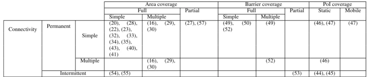
Table 2 provides a classification of the deployment algorithms studied in this survey. For each of them we give the coverage and connectivity problem addressed. Notice that we use the same classification criteria as in Table 1 of Section 1.2.
3 Analysis criteria of deployment algorithms
In this section, we analyze the different factors which have a positive or negative impact on the deployment. We discuss
7
Area coverage Barrier coverage PoI coverage Full Partial Full Partial Static Mobile Simple Multiple Simple Multiple
Connectivity Permanent (20), (28), (22), (23), (16), (29), (30) (27), (57) (49), (50) (52) (49) (46), (47) (47) Simple (32), (33), (34), (35), (43), (40), (41) Multiple (16), (29), (30) (52) (46) Intermittent (54), (55) (53) (44), (45)
Table 2 Classification of deployment algorithms.
the common assumptions and models found in the literature before focusing on the relationship between the sensing range, r, and the communication range, R, which highly impact the behavior of the deployment algorithm. Moreover, we define performance criteria for evaluation purposes. We end this section by highlighting the salient features of representative deployment algorithms.
3.1 Factors impacting the deployment
Several factors impact the deployment provided and determine how satisfactory the application is. They concern:
• The assumptions and models used concerning r the sensing range and R the communication range. Such assumptions and models are discussed in the next section. The discrepancy between these oversimplified models and reality may explain why the results obtained are not those which might be expected. The values of r and R determine the minimum number of sensors needed to fully cover the entity monitored (i.e. area, barrier or PoI). The deployment algorithms that use exactly this number are said to be optimal. Depending on the relationship between r and R, detailed in Section 3.3, some algorithms either work or not. Others are valid whatever the relationship between r and R, but are not, however, optimal in all cases.
• The number of sensor nodes available for the deployment and the dimensions of the entity monitored will determine whether this number is sufficient to fully cover the entity monitored. It is usually assumed that this entity has a regular shape (e.g. rectangle, disk, etc). However, the reality is often more complex with irregular borders.
• The sensor nodes’ ability to move is a determining factor. If sensor nodes are unable to move, the only possible deployment is an assisted one, where a mobile robot for example is in charge of placing the static sensor nodes at their final location. Otherwise, self-deployment is done, where each sensor node is autonomous and able to move. Notice that in such a case, the sensor nodes’ movement will consume more energy than communication during the deployment.
• The initial topology may require some extensions to the deployment algorithm. For instance, if the initial topology comprises several disconnected components and a centralized deployment algorithm is used, a mobile robot should be used to collect the initial positions of the nodes needed by the centralized deployment algorithm to compute the final positions of these nodes and this information should be disseminated to them. If on the other hand, a distributed
deployment algorithm is chosen, this algorithm should include a neighborhood discovery phase as well as a spreading phase to allow sensor nodes to quickly discover other connected components.
• The energy of sensor nodes is difficult or impossible to renew, and this fact is of great importance. In the deployment phase, the main reason for energy consumption is the movement of the nodes, whereas in the data gathering phase it is communication between the nodes. In both phases, energy-efficient techniques must be used.
• The presence of obstacles makes the deployment more complex: no sensor node should be placed within an obstacle. Hence, the obstacles must be detected and a strategy must be used by the deployment algorithm to get around the obstacles. Furthermore, if the shape of the entity monitored is complex with irregular borders, some extensions to the deployment algorithm will be needed.
• The quality of the data gathering required by the application may lead to a uniform and regular deployment. Such a deployment provides smaller data gathering delays (9), a better time and space consistency of the data gathered, which leads to a more accurate snapshot of the measures taken.
• The positioning system may introduce some inaccuracy in the position of the nodes; such a positioning error is very common with GPS. To meet the application requirements, the deployment algorithm should not accumulate the positioning errors during the deployment.
3.2 Common assumptions and models
The common assumptions and models found in the literature concern:
• Communication:
− A unit disk graph model is generally adopted, where any two nodes whose Euclidean distance from each other is less than or equal to the communication range R, have a communication link: they are able to communicate in both directions. This binary model is, however, too simple and does not match the real world. Some authors have introduced more complex models where the probability of success falls less abruptly when the distance increases up to R (10).
− A consequence of the unit disk graph model is that any wireless link is assumed to be symmetric. This assumption is not always true in the real world.
− A frequent assumption is that all sensor nodes have the same communication range. Sensor nodes may differ
8
in their age, their manufacturer, and their communication capacity. Hence some sensor nodes may have a higher transmission range than others.
− The initial topology considered in centralized deployment algorithms is usually connected with the sink. This may not be the case in the real world (see the discussion in Section 3.1). In distributed deployment algorithms, the initial topology is generally random, as it facilitates the spreading of nodes, leading to shorter convergence delays. For instance Figure 6a depicts an initial topology where some sensor nodes are unable to communicate with the sink. In addition, Figure 6b depicts another initial topology where all the sensor nodes are grouped at an entry point but unable to communicate with the sink.
a Random Topology. b Entry point topology.
Figure 6: Intial disconnected topology.
• Sensing:
− A unit disk graph model is used to model the sensing of a sensor node. Any event occurring within the disk of radius the sensing range r, centered at the sensor node is detected. This assumption is too optimistic in the presence of obstacles, for instance.
− The homogeneity of sensors (i.e. the same sensing model with the same sensing range) is generally assumed. This may not be the case in the real world.
• The presence of obstacles:
− Most authors assume that the entity to monitor is flat and nodes can move freely without obstacles. Such an assumption cannot be made for rescue applications after a disaster, for instance.
In the next section, we study the relationship between r and R in more detail.
3.3 Relationship between coverage and connectivity
Some deployment algorithms only work when a given relationship exists between the radio range R and the sensing range r. For instance, if R ≥ 2r, it is sufficient to ensure full coverage, and connectivity will be provided as a consequence. In the following, we study the different cases considered in the literature. Furthermore, we recall some results concerning optimal deployments based on regular patterns.
3.3.1 Sensor deployment algorithms based on the
relationship between R and r
• Case R ≥ 2r: Full coverage implies connectivity In (11) and (12), the authors prove that when R ≥ 2r the full coverage of a convex area implies full network connectivity. This result is extended to k-coverage and k-connectivity in (12). Then, using this assumption, it is sufficient to ensure full coverage, and connectivity will be a consequence.
• Case R ≥√3r: Full coverage implies connectivity In (13), it is proved that when R ≥√3r, ensuring full coverage implies full connectivity. Moreover, the number of sensors needed is optimal, when the triangular lattice is used as a deployment pattern. For instance, in (22), the authors propose a deployment algorithm where each sensor node should be placed in a vertex of an equilateral triangle of edge√3r.
• Case R = r
An optimal deployment algorithm is proposed in (16) to ensure full coverage and 1-connectivity when R = r. In this algorithm, sensor nodes are deployed along an horizontal line, each two neighboring nodes are at a distance of r. Adjacent lines are at a distance of (
√ 3
2 + 1)r. In such a deployment, full
coverage is ensured but only sensor nodes located in the same line are connected. That is why the authors propose adding a sensor node between each two adjacent lines in order to connect them, such that these nodes form a vertical line. Then 1-connectivity is ensured. The optimality of this deployment in terms of the number of sensor nodes was proved in (13).
• Case R <√3r
When R <√3r, full coverage does not imply network connectivity. Network connectivity is necessary to report information and it is an important part of the monitoring task. Then, ensuring connectivity while maximizing the area coverage becomes the goal of the deployment algorithm. The deployment algorithm proposed in (16) which deploys sensor nodes in horizontal lines and connects these lines by placing sensor nodes between two adjacent lines, is generalized in (13) as illustrated in Figure 7. In addition, this deployment is optimal when the distance between neighboring sensor nodes in the same line R and the distance between two adjacent lines is r +
q r2−R2
4 .
• Case arbitrary R and r
In (27), the authors propose an algorithm that aims at preserving network connectivity while maximizing area coverage. Starting with an initial deployment where all sensor nodes are connected to the sink, a virtual force algorithm is applied in order to redeploy sensor nodes in the area considered. As the sensing and radio ranges do not meet the assumption R ≥√3r, when sensor nodes move to their new positions they check whether they are still connected to the sink. If they are not, they move towards the sink
9
Figure 7: Sensor deployment with added sensors to ensure connectivity.
until connectivity is established. This algorithm preserves full network connectivity during the deployment process and tries to maximize the area coverage with any given values of R and r. In (20), the authors propose a deployment algorithm that aims at ensuring full coverage and full network connectivity of an area containing obstacles of different shapes. The authors propose dividing the area into two different types of region: small regions or large regions which can contain boundaries and obstacles. As there are no assumptions concerning R and r, in the small regions (like a belt), sensors are deployed along the bisectors of this region and are separated by rmin=
min{R, r}. In the large region, sensor nodes are deployed in rows. The distances which separate sensor nodes and rows are determined according to the values of R and r.
3.3.2 Optimal number of sensor nodes for regular
deployment patterns
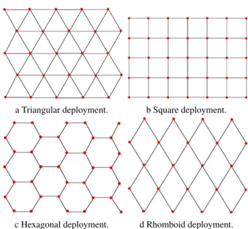
Sensor nodes can be deployed in a regular pattern. This pattern can be a triangular lattice, a square grid, an hexagonal grid or a rhomboid grid. In (5), the authors specify for each pattern a condition that ensures coverage of the area and guarantees network connectivity as a consequence.
• If R ≥ r and the hexagonal grid pattern is used, then full area coverage is ensured and the network is connected. • If R ≥√2r and the square grid or rhomboid pattern is
used, then full area coverage is ensured and the network is connected.
• if R ≥√3r and the triangular lattice pattern is used, then full area coverage is ensured and the network is connected. The triangular lattice is the optimal deployment pattern to ensure full area coverage and guarantee network connectivity.
These conditions are studied in (13) with regard to the optimal number of sensor nodes and the regular pattern used. It was proved that when:
• 0 < Rr ≤ 1 23
3/4, the hexagonal grid is the best
deployment pattern (i.e. it requires the minimum number of sensor nodes). See Figure 8c.
a Triangular deployment. b Square deployment.
c Hexagonal deployment. d Rhomboid deployment.
Figure 8: Regular deployment pattern.
• 1 23
3/4≤R r ≤
√
2, the square grid is the best deployment pattern. See Figure 8b.
• √2 ≤ R r ≤
√
3, the rhomboid pattern is the best deployment pattern. See Figure 8d.
• Rr ≥√3 the triangular lattice is the best deployment pattern. See Figure 8a.
3.4 Criteria for performance evaluation
Each pattern may fit some application requirements. The question is then how to evaluate and select the best one. Different evaluation criteria have been introduced:
• coverage: (e.g. area, barrier, point of interest) is the main criteria to evaluate the efficiency of the algorithm. Usually, coverage is computed as follows: the area to cover is divided virtually into LxW grid units. A grid unit is considered to be covered if and only if its centered point is covered by at least one sensor node. The coverage rate is computed as the percentage of grid units covered.
• connectivity: is also important. The type of connectivity (e.g. full or intermittent) is application dependent. For some applications, maintaining full connectivity is required in order to report any detected event immediately to the sink. Other applications with fewer constraints require intermittent connectivity: usually a data mule.
• convergence and stability: convergence is evaluated by the convergence time defined as the time needed to achieve the required coverage and connectivity. In distributed deployment algorithms, the convergence may be difficult to reach because of node oscillations. Hence, the stability of the deployment is an important criterion to detect the completion of the deployment.
• energy and distance traveled: during the deployment, the main cause of energy consumption is the mobility of the
10
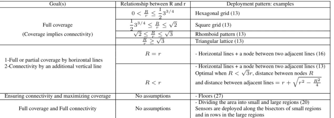
Goal(s) Relationship between R and r Deployment pattern: examples 0 <R r ≤ 1 23 3/4 Hexagonal grid (13) Full coverage 1 23 3/4≤R r ≤ √ 2 Square grid (13) (Coverage implies connectivity) √2 ≤R
r ≤ √ 3 Rhomboid pattern (13) R r ≥ √ 3 Triangular lattice (13)
R = r - Horizontal lines + a node between two adjacent lines (16) 1-Full or partial coverage by horizontal lines
2-Connectivity by an additional vertical line - Horizontal lines + a node between two adjacent lines (13) Optimal when R <√3r, distance between nodes R R < r and distance between adjacent lines = r +
q r2−R2
4
Ensuring connectivity and maximizing coverage No assumptions - Floors (27)
- Dividing the area into small and large regions (20) Full coverage and Full connectivity No assumptions Sensors are deployed along the bisectors of small regions
and in rows in the large regions
Table 3 Relationship between r and R.
nodes. That is why the total distance traveled by the nodes must be measured, as this measure reflects the energy consumed. Obviously, minimizing the total distance traveled leads to savings in energy. Notice that the convergence and stability performance has a strong impact on the distance traveled and the energy consumed. Once the deployment has been carried out and the nodes are stationary, the data gathering takes place. The main cause of energy consumption in this phase is communication. To maximize network lifetime, node activity scheduling can be used to make nodes sleep when they are not needed for the data gathering.
• communication overhead: comes from the control messages exchanged between the nodes to organize the deployment and the data gathering. In the case of contention-based medium access, collisions imply retransmission and increase the overall bandwidth and energy consumption. The aim is to reduce this overhead.
• uniformity, regularity and optimality of the deployment: if the space consistency of measures taken is expected, a uniform deployment is needed: all the nodes (except the border ones) should have the same number of neighbors. Similarly, if the measures should be taken at equidistant positions, a uniform and regular deployment is needed. Usually, such a deployment reproduces the same geometric pattern (e.g. triangle, hexagon, square , etc). Depending on the relationship between r and R, some patterns are optimal. This optimality is useful because it requires the smallest number of sensor nodes to meet the application requirements. A uniform and regular deployment is also mandatory when the application requires time and space consistency of the data gathered.
3.5 Salient features of deployment algorithms
For each protocol studied, we define the coverage and connectivity problem solved, the strategy used, its type (centralized, distributed) and its specific assumptions. For area coverage, we distinguish different strategies that are detailed in Sections 4, 5 and 6 for area, barrier and PoI coverage, respectively.
4 Area coverage and connectivity algorithms
4.1 Full coverage
Many deployment algorithms aim to ensure full coverage of the area considered. These algorithms are classified into three strategies. We distinguish the forces-based strategy, the grid-based strategy and the computational geometry-grid-based strategy.
4.1.1 Forces-based strategy
The forces-based strategy is known by its simple deployment principle. This principle is based on virtual forces that can be attractive, repulsive or null. In this strategy, a sensor node should maintain a fixed threshold distance called Dth with
its 1-hop neighbors. Then, if the distance separating two neighboring nodes is greater than Dth, an attractive force is
exerted, whereas if this distance is less than Dth, a repulsive
force is exerted. Otherwise, the force is null since the distance separating neighboring sensor nodes is equal to Dth, the
required distance. This principle is illustrated in Figure 9, where−→Fijdenotes the force exerted by sensor node j on sensor
node i.
11
Area coverage
Protocol Coverage problem Connectivity problem Strategy Cent/Dist Specific assumptions VFA (21) Full coverage Permanent connectivity Forces based Centralized
Extended VFA(24) Full coverage Permanent connectivity Forces based Distributed R
r > 2.5 and R r < 2.5
IVFA (25) Full coverage Permanent connectivity Forces based Distributed EVFA (25) Full coverage Permanent connectivity Forces based Distributed
DVFA (22) (23) Full and uniform coverage Permanent connectivity Forces based Distributed R ≥√3r CPVF (27) Maximized coverage Permanent connectivity Forces based Distributed arbitrary R and r Push&Pull (28) Maximized coverage Permanent connectivity Forces based Distributed Triangular lattice
Forces based Square grid VFCSO(26) Full coverage Full connectivity Grid based Centralized R ≥√5r
Node activity scheduling (29) Full coverage Permanent connectivity Grid based Distributed
Multiple Multiple
(30) Full coverage Permanent connectivity Grid based Distributed Multiple Multiple
HGSDA(32) Full coverage Permanent connectivity Grid based Centralized Triangular lattice R ≥√3r C2 (34) Full coverage Permanent connectivity Grid based Distributed Triangular lattice
Energy saving (33) Full coverage Permanent connectivity Grid based Distributed Square pattern Square pattern (35) Full coverage Permanent connectivity Grid based Distributed Static node
Assisted by robot (56) Partial coverage Permanent connectivity Grid based Cent/Dist
VEC, VOR and Maximized coverage Permanent connectivity Computational Distributed Voronoi diagram
Minimax (40) geometry based
(43) Full coverage Permanent connectivity Computational Centralized Delaunay triangulation geometrie based Obstacles
(41) Full coverage Permanent connectivity Computational Centralized Static nodes geometry based
Robot collector (54) Full coverage Intermittent connectivity Random Centralized Cluster head
Energy saving (55) Full coverage Intermittent connectivity Random Centralized Ferries
(15) Full coverage Permanent connectivity Random Distributed Node activity scheduling (17) Full coverage Permanent connectivity Random Centralized Node activity scheduling Connected graph based (12) Full coverage Permanent connectivity Random Distributed R ≥ 2r
Simple-Multiple Node activity scheduling (19) Full coverage Permanent connectivity Random Distributed Arbitrary R and r
Node activity scheduling (57) Partial coverage Permanent connectivity Random Dist/Cent Node activity scheduling
Barrier coverage
Protocol Coverage problem Connectivity problem Strategy Cent/Dist Specific assumptions (49) Full coverage Permanent connectivity Grid based Distributed Mobile sensors
Simple-Multiple
(50) Full coverage Permanent connectivity Random Centralized Random offset < r (51) Full coverage Permanent connectivity Random Centralized
MBC (52) Full coverage Permanent connectivity Deterministic Distributed R ≥ 2r
Simple-Multiple Dynamic object
CSP (53) Partial coverage Intermittent connectivity Probabilistic Centralized PMS (53) Partial coverage Intermittent connectivity Probabilistic Centralized
(59) Full coverage Permanent connectivity Random Centralized Node activity scheduling
Point of Interest coverage
Protocol Coverage problem Connectivity problem Strategy Cent/Dist Specific assumptions (47) Full coverage Permanent connectivity Forces based Distributed RNG for connectivity
Static PoI (44) Temporary coverage Intermittent connectivity Random Distributed Ferries
R ≥ 2r DSWEEP (45) Temporary coverage Intermittent connectivity Distributed
(46) Full coverage Permanent Connectivity Grid based Distributed R ≥√3r
12
The virtual forces algorithm (VFA) is proposed in (21) as a centralized redeployment algorithm to enhance an initial random deployment. In the initial deployment, any sensor node is able to communicate with the sink in a one-hop or multi-hop manner. Then, the sink computes the appropriate new position of each sensor node based on the coverage requirements and using the virtual forces mechanism. In this work, obstacles exert a repulsive force and an area of preferential coverage exerts an attractive force on sensor nodes. During the execution of the virtual forces algorithm, sensor nodes do not change their positions. It is only when they receive their final positions from the sink that they move directly to them. VFA is a centralized algorithm that offers a good coverage rate of the area considered while maintaining network connectivity. However, a central entity must know the initial positions of all sensor nodes, compute their final positions and disseminate the positions to all sensor nodes. This principle is problematic when network connectivity is not initially ensured. Furthermore, when the network is very dense, this algorithm has a poor performance due to the gathering of the initial positions of sensor nodes.
To cope with the scalability problem, distributed versions of VFA are proposed in the literature. For instance, the extended virtual forces-based approach proposed in (24) copes with two drawbacks of the virtual forces algorithm: the connectivity maintenance and nodes stacking problems (i.e. two or more sensor nodes occupy the same position). The connectivity maintenance problem occurs when the communication range is low, Rr < 2.5. Thus, the authors propose adding an orientation force which is exerted only if the node has fewer than 6 neighbors. This force aims to keep the angle formed by one node and its two neighbors equal to
π
3 in order to provide a reliable connectivity and eliminate
coverage holes. Notice that these authors observe a stacking problem, where several nodes are located in almost the same position. This is because the coefficient of the attractive forces is not well tuned. As a solution, the authors propose an exponential force model to adjust the distance between a node and its distant neighbors. However, the threshold value of Rr = 2.5 is not explained and the maintained connectivity is not proved in the paper. Furthermore, the additional orientation force may induce node oscillations.
IVFA, Improved Virtual Force Algorithm, and EVFA, Exponential Virtual Force Algorithm are two distributed deployment algorithms proposed in (25). EVFA aims at speeding up convergence because forces increase exponentially with the distance between sensors. IVFA limits the scope of virtual forces: only nodes in radio range of a given node exert virtual forces on it. Furthermore, the stacking problem is solved by using a very small attractive force with regard to the repulsive force. IVFA converges to a steady state faster than the basic virtual forces algorithm, and defines a maximum movement in each iteration to reduce useless moves and save energy.
DVFA, proposed in (22), is another example of the distributed algorithm that uses the virtual forces to spread sensor nodes until the entire area is covered. The main drawback of this algorithm is node oscillations. To deal with this problem, the authors of DVFA limit the distance sensor nodes move to a
certain threshold. In this way, energy consumption is reduced during the deployment which provides a fast convergence to a coverage rate close to 100%. DVFA is also used in (23) to cope with obstacles of different shapes. By using the virtual forces principle and a method to avoid the obstacles, full area coverage is ensured even when an obstacle has a confined shape.
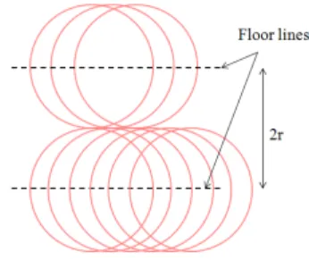
Usually, the virtual forces strategy is used to ensure full area coverage as the attractive and repulsive forces spread sensor nodes over the whole area and consequently achieve a high coverage rate rapidly. Furthermore, this strategy is used in (27) with the goal of preserving network connectivity. This deployment algorithm, called CPVF, Connectivity-Preserved Virtual Force, is used to monitor an unknown area with an arbitrary ratio Rr. To achieve that, a sink periodically broadcasts a message to neighboring sensors which in turn flood the message to all connecting nodes. A sensor node is considered to be disconnected from the network if it does not receive the flooding message. Then, it moves toward the sink in order to reconnect. This algorithm induces a high overhead in terms of messages broadcast in the network to check the connectivity of the nodes with the sink. This paper also proposes a floor-based scheme to improve the global network coverage by reducing overlapping. This scheme is based on the division of the area into equidistant floors (distant of 2r) and encourages sensors to stay in the floor lines. Sensor nodes are added in a column between floor lines to ensure connectivity. Although this work aims at preserving network connectivity when the ratio Rr is arbitrary, it requires a high number of sensor nodes, as illustrated in Figure 10, because the inter-floor distance is fixed to 2r for any value of R and r.
Figure 10: Floor based deployment.
4.1.2 Grid-based Strategy
The grid-based strategy provides a deterministic deployment where the position of the sensor nodes is fixed according to a special grid pattern such as a triangular lattice, a square grid or a hexagonal grid (see Figures 11b, 12 and 13 respectively). Then, the area is divided into virtual cells and depending on the deployment algorithm used, sensor nodes are located either in cell vertices or at the cell center.
The grid deployment is also a regular deployment pattern as all the generated grid cells have the same shape and
13 size. The regular deployment pattern is studied in (29) in
order to provide multiple coverage (p-coverage) and multiple connectivity (q-connectivity) using the triangular lattice, square or hexagonal pattern. The value of p and q are provided by adjusting the distance separating sensor nodes and limiting the ratio Rr. A comparative study of regular pattern performance in terms of the number of nodes required is also provided to achieve 1, 3 and 5-coverage and q-connectivity. With the ratioRr ≥√3, the triangular lattice is better than the square grid, which is better than the hexagonal grid. However, with the value of Rr <√3, the triangular lattice becomes the worst. Multiple coverage and connectivity with regard to the regular deployment pattern is also studied in (30). The authors propose the optimal deployment patterns to ensure full coverage and q-connectivity while q ≤ 6 for certain values of Rr. They consider the hexagonal deployment pattern as a universal basic pattern that can generate all optimal patterns. Then, they present different forms derived from the hexagonal pattern by changing the edge length and the angle between adjacent edges.
When the applications require time and space consistency of the measures taken by sensor nodes regularly distributed in the area, the regular deployment pattern can be a good solution to provide a high level of coverage and connectivity with a minimum number of sensor nodes.
In the following we present some research studies proposing a regular deployment pattern based on a triangular lattice and a square grid.
Triangular grid
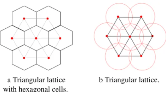
In (31), it was proved that the triangular lattice shown in Figure 11b offers the smallest overlapping area and requires the smallest number of sensor nodes. When the triangular lattice is used as a deployment pattern, each sensor node occupies a hexagonal cell. However, the deployment is not considered to be a hexagonal deployment (see Figure 13) since a sensor node is at the center of a hexagon and neighboring sensors form a triangular pattern (see Figure 11). For instance, the authors in (32) propose a deployment algorithm called HGSDA that deploys sensor nodes in a triangular lattice. This deployment starts by dividing the area into small hexagonal cells and each cell center corresponds to a sensor position. Although the cells are hexagonal, sensor nodes are deployed in a triangular lattice since the distance between two neighbors is√3r and there is a sensor node at the cell center. HGSDA identifies redundant sensor nodes in order to place them in empty hexagonal cells. Since the size of a hexagonal cell is computed according to sensor sensing range and the area size, full coverage is achieved using the smallest number of sensor nodes. This algorithm is carried out by a sink. Then, all the sensor nodes receive their final position from the sink and move to it. HGSDA is a centralized algorithm that ensures full coverage using the minimum number of sensor nodes while ensuring simple connectivity with the sink in the final deployment. This centralized algorithm can only be used if connectivity with the sink is ensured in the initial deployment. The same deployment pattern is presented in (28), but in a distributed version. However, at the beginning
a Triangular lattice with hexagonal cells.
b Triangular lattice.
Figure 11: Triangular lattice.
of the deployment, the area is not yet divided into hexagonal cells. An initiative sensor node starts by snapping itself at the center of the first hexagonal cell and selects six sensor nodes in its vicinity to snap them in the adjacent hexagonal cells. The selected sensor nodes move to their cells and in turn select other sensor nodes to occupy their adjacent cells. Then, hexagonal cells are built progressively in a distributed way: the hexagonal side length is equal to the sensing range. Since the sensor occupies the center of the cell, the triangular lattice is used as the deployment pattern.
The deployment algorithm C2proposed in (34) is a triangular lattice based strategy where a sensor node occupies a hexagonal cell. Hexagonal cells are built progressively in a distributed manner by sensor nodes. This algorithm proceeds in two phases. In the first phase, called cluster heads selection, the sink which is the first cluster head in the area considered, starts by building its hexagonal cell and defines its position as the cell center. The distance between the cell center and one of the vertices isR3 and the distance between two neighboring cell centers is 2R3 in order to maintain network connectivity during the deployment process. Then, the sink determines the center of each neighboring cell and informs sensor nodes in its neighborhood. The nearest sensor node to the cell center is selected as a cluster head of its hexagonal cell. It should move towards its cell center. In turn, the new cluster heads define the center of their neighboring cells. The second phase is called node balancing and its goal is to improve area coverage by balancing the number of sensor nodes between cells. To do so, if the difference between sensor nodes in two neighboring cells is greater than 1, some sensor nodes will move to the cells with a deficit number of nodes. In this deployment algorithm, a hexagonal grid is used to ensure full coverage and maintain full connectivity. Energy saving is achieved by selecting a cluster head for each cell and balancing the number of sensor nodes between adjacent cells. This algorithm performs well when the sink is located at the center of the area and all the nodes are grouped around the sink.
Square grid
The square grid strategy is used in (33) where the area monitored is divided into square cells, as shown in Figure 12. Each cell represents the maximum square size that is covered by one sensor node. Each sensor node occupies a cell center to cover the corresponding square cell. If an empty cell exists, neighboring sensor nodes should decide to which one will
14
move to cover it, such that if new empty cells appear, they will be around the sink. Redundant nodes should move toward the sink in order to cover empty cells that can occur along the path to the sink.
A grid-based approach is also used for robot-assisted sensor deployment. As an example in (35), a robot places sensor nodes at the vertices of a square cell. Then, each deployed sensor node colors itself white if it is adjacent to an empty cell and black otherwise. Neighboring sensor nodes exchange hello messages to inform each other about white nodes (empty cells) and maintain a back pointer corresponding to the nearest empty cell along the backward path of the robot. Then, the robot backtracks this back pointer to drop sensor node in the empty cell. This algorithm guarantees full coverage in a failure free environment using a mobile robot in a square grid.
It is assumed that the robot carries enough sensors to heal any coverage hole (i.e. empty cell) that is detected. Such strategies are used when the sensor nodes are static, and a mobile robot is used to ensure coverage by repairing any coverage hole detected by the sensor nodes. The new problem is that of detecting coverage holes and optimizing the robot movements.
a Sensors in the cell centers.
b Sensor in cell vertice.
Figure 12: Grid Based Strategy.
Figure 13: Hexagonal pattern.
4.1.3 Computational geometry based Strategy
The computational geometry strategy is used to solve problems based on geometrical objects: points, polygons, line segments, etc. Voronoi diagram and Delaunay triangulation are two computational geometry methods used in WSNs to solve static problems. The Voronoi diagram is a method
of partitioning the area into a number of polygons based on distances to a specific discrete set of nodes. Each node occupies only one polygon and is closer to any point in this polygon than any other node in the neighboring polygons. These polygons can be obtained by drawing the mediator of each two neighboring nodes. Consequently, the edges of the polygons are equidistant from neighboring nodes. Delaunay triangulation is the dual graph of the Voronoi diagram. It can be constructed by connecting each two neighboring points in the Voronoi diagram whose polygons share a common edge. Voronoi diagram and Delaunay triangulation are used in WSNs to deal with coverage hole problems. The occurrence of coverage holes after the deployment of sensor nodes in a given area can be considered as a cause of a low coverage rate. By detecting and healing these holes, the coverage rate can be maximized.
Deployment algorithms based on Voronoi diagram
Some schemes proposed are based on Voronoi diagram to detect coverage holes. Sensor nodes are able to construct their Voronoi polygons based on location information received from their neighbors. Due to these Voronoi polygons, nodes can determine coverage holes. Then, they move in order to reduce or eliminate these holes while maximizing the coverage rate of the area considered.
In (40), three distributed moving algorithms are proposed: VEC, VOR and Minimax algorithms. The VECtor based algorithm (VEC) is inspired by the behavior of electromagnetic particles. When two electromagnetic particles are too close to each other, an expelling force pushes them apart. VEC pushes sensor nodes away from a densely covered area. In contrast to the VEC algorithm, the VORonoi based algorithm (VOR) pulls sensor nodes to the sparsely covered area. The Minimax algorithm is similar to VOR. It fixes coverage holes by moving sensor nodes closer to the furthest Voronoi vertex. However, it does not go as far as VOR to avoid situations in which a vertex that was originally closer now becomes the furthest. Minimax chooses the node target position as the point inside the Voronoi polygon whose distance to the furthest Voronoi vertex is minimized. Minimax and Vor do not ensure uniform coverage of the final deployment since the algorithm stops as soon as full coverage is obtained. Moreover, if the number of sensors is not sufficient to cover the whole area, node oscillations may occur.
Deployment
algorithms
based
on
Delaunay
Triangulation
In (43), a centralized algorithm is proposed to cope with the boundaries and obstacles coverage problem. In their paper, the authors propose a deterministic sensor node placement to ensure full coverage of an area containing obstacles of arbitrary shapes. Sensor nodes are deployed in a triangular lattice over the whole area as if there were no obstacles. Then, sensor nodes inside the obstacles are eliminated and
15
a Voronoi diagram. b Delaunay triangulation.
Figure 14: Computational geometry approach.
so coverage holes may occur around these obstacles. To deal with this problem, Delaunay triangulation is used to partition these coverage holes into triangles of edges less than r, and then, a sensor node is placed in one of the triangle vertices to cover it.
Other computational geometry deployment algorithms
Another study based on computational geometry strategy is proposed in (41) to detect any coverage hole and calculate its size. In this work, the authors do not rely on Voronoi diagram or Delaunay triangulation, but, they propose a triangular oriented diagram called HSTT that connects static sensor nodes such that every three neighboring nodes form a triangle. Using a HSTT diagram, coverage holes can be detected and the required number of mobile sensors to heal these holes can be determined. Although this HSTT diagram presents some advantages compared to a Voronoi diagram, such as its simplicity and its accuracy when computing the size of the coverage holes, it requires a high energy consumption to achieve its goal.
4.1.4 Other deployment strategies
Other deployment strategies exist. They include off-line optimization algorithms which compute off-line the best position of each sensor node with the goal of ensuring the coverage and connectivity required by the application. For this purpose, they employ optimization techniques, usually based on a linear programming of the problem considered. They discretize the area of interest and decide for each point in the area whether a sensor should be located there or not, taking into account the application requirements (e.g. maximum number of sensors, maximum cost, etc). See for instance (42).
4.2 Partial coverage
The area coverage problem has been widely studied in the literature. As we have shown previously, much effort has been made to cope with full area coverage. However, only a few studies have focused on partial area coverage.
Generally, partial coverage is a solution to prolong the network lifetime when full coverage is not required. The foremost requirement in this case is that the coverage rate provided should be higher than some predefined bound which is a
a A large uncovered area. b Regular distribution of uncovered area.
Figure 15: Partial coverage.
a Bad distribution. b Good distribution.
Figure 16: Different distributions of uncovered area.
specific parameter fixed by the application. The goal is to cover at least θ percent of the area considered while maintaining a connected graph between these nodes. Partial coverage is useful to measure the temperature and humidity, to detect smoke and to provide an early warning of a potential forest fire (58), for instance.
In addition, to avoid a large uncovered area (see Figure 15a), the uncovered areas should be regularly distributed (see Figure 15b). For that purpose, the authors in (56) propose dividing the area to be monitored into subregions of equal size. The goal is then to cover θ-percent of each subregion.
4.3 Intermittent connectivity
The deployment algorithms presented above ensure full or partial coverage with permanent connectivity. When permanent connectivity is not required, intermittent connectivity is provided, exploiting the mobility of some nodes. The strategies differ in:
• the number of mobile nodes: one mobile node or several. If several, how do the mobile nodes coordinate their action to visit nodes and gather their data?
• the trajectory type of mobile nodes:
– a fixed predefined geometrical trajectory like a line or a circle, for instance.
– a trajectory that visits all the nodes or a subset of nodes depending on the deployment architecture (e.g. clustering).