Musical genre descriptor for classification based on Tonnetz trajectories

HAL Id: hal-03031287

https://hal.archives-ouvertes.fr/hal-03031287

Submitted on 30 Nov 2020

HAL is a multi-disciplinary open access

archive for the deposit and dissemination of

sci-entific research documents, whether they are

pub-lished or not. The documents may come from

teaching and research institutions in France or

abroad, or from public or private research centers.

L’archive ouverte pluridisciplinaire HAL, est

destinée au dépôt et à la diffusion de documents

scientifiques de niveau recherche, publiés ou non,

émanant des établissements d’enseignement et de

recherche français ou étrangers, des laboratoires

publics ou privés.

Tonnetz trajectories

Emmanouil Karystinaios, Corentin Guichaoua, Moreno Andreatta, Louis

Bigo, Isabelle Bloch

To cite this version:

Emmanouil Karystinaios, Corentin Guichaoua, Moreno Andreatta, Louis Bigo, Isabelle Bloch. Musical

genre descriptor for classification based on Tonnetz trajectories. Journées d’Informatique Musicale,

Oct 2020, Strasbourg, France. �hal-03031287�

MUSIC GENRE DESCRIPTOR FOR CLASSIFICATION BASED ON

TONNETZ TRAJECTORIES

Emmanouil Karystinaios

Corentin Guichaoua

Moreno Andreatta

Louis Bigo

Isabelle Bloch

1

_{Université Paris Diderot}

2

_{STMS, CNRS,}

IRCAM, Sorbonne Université

3

_{IRMA, CNRS,}

Université de Strasbourg

4

_{CRIStAL, CNRS}

Université de Lille

_{LTCI, Télécom Paris}

Institut Polytechnique de Paris

manoskaristineos@ gmail.com corentin.guichaoua@ircam.fr andreatta@math.unistra.fr louis.bigo@univ-lille.fr isabelle.bloch@ telecom-paris.fr RÉSUMÉ

Dans cet article, nous présentons un nouveau descrip-teur pour la classification automatique du style musical. Notre méthode consiste à définir une trajectoire harmo-nique dans un espace géométrique, le Tonnetz, puis à la résumer à ses valeurs de centralité, qui constituent les des-cripteurs. Ceux-ci, associés à des descripteurs classiques, sont utilisés comme caractéristiques pour la classification. Les résultats montrent des scores F1supérieurs à 0,8 avec

une méthode classique de forêts aléatoires pour 8 classes (une par compositeur), et supérieurs à 0,9 pour une classi-fication en 4 classes de style ou période de composition.

1. INTRODUCTION

Genre classification of music is an important branch in Music Information Research (MIR). Usually, symbo-lic music classification, as opposed to audio-based ap-proaches, mainly relies on general descriptors for MIDI specifications and general statistics, such as the lowest and highest notes, maximum repetition of chords or notes, etc., rather than harmonic characteristics of symbolic scores. Stylistic classification, in particular, is mainly developed on monophonic streams [10]. In this article, we propose a new approach for stylistic music classification, driven by chord material.

The main issues of polyphonic music classification are the representation and the reduction of the data. For instance, some approaches choose to convert polyphonic extracts to multiple monophonic streams [18] or choose a restricted alphabet to only represent certain types of chords [7]. While automatic harmonic analysis seems promising, with methods such as jSymbolic [25] and Sty-lerank[13], there are some imposed restrictions such as the filtration of chords based on duration, persistence, type, size and rhythmic positioning.

In this paper, we present a novel approach without vo-cabulary restrictions on the chord material but rather an evaluation of the total harmonic content. Following Louis

Bigo’s approach on trajectories in generic simplicial com-plexes [4], we also make use of the Tonnetz in order to represent the musical data. A compliance function selects the appropriate Tonnetz for the considered chord material. In this Tonnetz we build a harmonic trajectory of the MIDI piece based on some core principles and different case by case strategies. This trajectory is then reduced to a limi-ted number of values which are used for the classification process.

For classification, we suggest basic supervised me-thods such as Random Forest and k-Nearest Neighbors (used here in a supervised way). Furthermore, we present experiments for binary and multi-class versions of clas-sification. The binary classification utilizes only the tra-jectory descriptor values, whereas the multi-class version makes use of other simple descriptors as well, for optimal performance.

2. TRAJECTORY AND DERIVED DESCRIPTORS The core of the proposed approach is described in this section. Assuming that harmony is one of the most im-portant parameters in determining the style of a musical piece, the main idea is to transform a series of chords in a spatial trajectory in an appropriate space, and then derive descriptors from this trajectory.

From a midi file, chords are extracted using music21 tools [12], and in particular the function chordify.

The next step is to define how to build a trajectory. Ac-cording to Bigo, a trajectory is defined in a pitch space called Tonnetz [4]. The Tonnetz is defined as a spatial organization of musical pitches, along three axes, where every axis is based on a given interval. A Tonnetz will then simply be denoted by these three intervals, e.g., T (3, 4, 5) meaning that the axes represent minor thirds, major thirds and perfect fourths (and their complementary intervals).

In this article, we use the term Tonnetz in the sense of a graph which is not bound (i.e. an infinite grid). Let v be a vertex in this graph. The neighbors of v are defined by the intervalic relations of the selected Tonnetz. Every vertex

has 6 neighbors defined by the 3 Tonnetz intervals and their complement modulo 12. In our approach, we use the well-tempered 12-semitone system so that we can handle chords and harmony. Note that one could use a different tempered system with smaller or larger intervals.

We do not use all 12-note Tonnetze but only the five which have the topological structure of a torus, as origi-nally characterized in [9] and studied in details in [21]. This means that we exclude the non-connected Tonnetze on which finding a compact and connected trajectory would often be impossible.

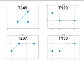
Let us provide some examples. Considering the Ton-netz T (3, 4, 5), a spatial representation can be defined on a square grid, and T would be represented by associating the interval 4 (i.e. a major third) to the x-axis, and the interval 3 to the y-axis. The interval 5 would then be re-presented on the diagonal. A 4 × 3 size grid is then per-iodically repeated. In a similar way T (1, 3, 8) will be re-presented with interval 8 on the x-axis and 3 on the y-axis. These examples and others are displayed in figure 1, where a C major chord is represented on four Tonnetze.

Figure 1. The representation of a C major chord, i.e. the pitch class set Cmaj = {0, 4, 7}, in four different Ton-netze. The notes of the chord are illustrated in blue. The intermediate edges and notes (connecting the chord repre-sentation) are denoted in red. The note C = 0 is always placed at point (0, 0).

2.1. Trajectory

The trajectory is defined as a path X in the Tonnetz T , i.e. an ordered list of positions in the space T .

Let us investigate some basic scenarios for trajectory construction. Placing the first note in the Tonnetz has no bearing on the descriptors we ultimately compute, so we can simply pick an arbitrary position. Now we consider the case where we have to place two notes : one of them is placed as in the previous case, and the second one is pla-ced according to a criterion depending on a distance mea-sure. To this end, we define a function dist : Z12× Z12→

N, which assigns to the pitch class representation of notes,

x and y, their distance according to a given Tonnetz as :

dist (x, y) =      0 if x = y 1 if (x − y) ∈ T ∨ (y − x) ∈ T 2 otherwise (1)

Note that dist (x, y) = dist (y, x). By abuse of notation, from now on when referring to notes or chords we auto-matically consider the numerical representations of their pitch class (PC). They are defined with integer notation, where C = 0, C] = 1, D = 2, etc. Accordingly, chords are PC sets.

Two notes x, y are neighbors if dist (x, y) = 1. Thus, in the case where two notes are neighbors we find which kind of interval they form and to which Tonnetz axis this interval corresponds. In the case where dist (x, y) = 2, we define a positioning according to a shared neighbor. For example, in Tonnetz T (1, 2, 9), the placement of note E in relation to note C is computed using the shared neighbor D : D is first placed in relation to C, then E is placed in relation to D. This example is illustrated in figure 1 (horizontal axis). The intermediate neighbors are denoted in red.

Given a note x, a position p and a fixed Tonnetz T , let π(x, p) be a positioning function for T which, from the reference position p, places the note x as described above. We now move on to chords, which we will demons-trate on the simple case of a triad but generalize as well to chords of any size. In figure 1 a C major chord is re-presented in 4 different Tonnetze, T (1, 3, 8), T (1, 2, 9), T (3, 4, 5) and T (2, 3, 7). From this representation we can see that in T (3, 4, 5) the chord forms a connected graph while in the other cases the graph is disconnected. In all representations, we place the note C = 0 at point (0, 0). From there, we place the other notes based on the Ton-netz intervals and periodicity. For example, we first need to find whether E and G are neighbors of C in Tonnetz T . For this we consider the following function, which gives the neighbors of note y in the chord X according to Ton-netz T :

neigh(y, X, T ) = {x ∈ X | dist (y, x) = 1 in T } (2) In the C major scenario, E and G are neighbors of C in Tonnetz T (3, 4, 5) so we can easily find their place in T . We define a function which takes a chord X and a position p in a fixed space T and assigns positions to all notes of X as follows :

f (X, p) = {π(x, p) | x ∈ X} (3) If a chord does not strictly consist of neighboring notes, we first place notes which are neighbors of y, then we at-tempt to place the remaining notes according to the newly positioned notes, repeating until no more notes can be pla-ced. If some notes remain to be placed, then one of the re-maining notes is placed in relation to an arbitrary already placed note, and the process is repeated. This process is summarized in algorithm 1.

Algorithm 1: Placement of the first chord Input: (X, T ) Result: placed Let x ∈ X, pxarbitrary; placed = {(x, px)} ; to_place = X \ {x} ; while to_place 6= ∅ do

while ∃(x, px) ∈ placed, ∃y ∈ to_place such

thaty ∈ neigh(x,to_place, T ) do placed = placed ∪{(y, π(y, px))} ;

to_place = to_place \{y} ; end

let y ∈ to_place, (x, px) ∈ placed :

placed = placed ∪{(y, π(y, px))} ;

to_place = to_place \{y} ; end

This process analyzes in depth the method for positio-ning chords with a starting reference point. Given a chord X and a Tonnetz T we now know how to place all notes of X in T . The natural question is how to generalize the previous construction to the case of a sequence of chords. Let us consider the simplest case with two chords X, Y . We know the positions for all elements of X and we want to find a reference note and point to find the positions of the elements of Y . We need to find the best candidates y0 ∈ Y and x0 ∈ X to find a position for y0. We remind

that the position px0of x0is known. We set :

y0= argmin y∈Y

X

x∈X

dist (x, y) (4)

i.e. the note achieving the minimum ofP

x∈Xdist (x, y), and similarly : x0= argmin x∈X X y∈Y dist (x, y) (5)

These are the best candidates of the two chords, and a po-sition for y0 is then obtained by the function π(y0, px0).

The rest of the chord is then placed according to the main loop of algorithm 1. We note u(Ci, Cj, Pi) the function

that assigns positions to the chord Cj based on chord Ci

and its positions Pi.

Although this method ensures termination, it is not fully satisfying as it does not guarantee the most compact representation for a larger sequence of chords.

Let [C1, ..., Cn−1, Cn, Cn+1, ..., Ck] be a list of chords.

Suppose that for the chords C1, ..., Cn−1 the

correspon-ding positions P1, ..., Pn−1 are known and we search

a position for the chord Cn. We propose a method for

considering two different positions for chord Cn and a

verification system for checking the compactness of the solution. Let us define

P_n0 = u(Cn−1, Cn, Pn−1) (6)

P_n+1# = u(Cn−1, Cn+1, Pn−1) (7)

P_n00= u(Cn+1, Cn, Pn+1# ) (8)

Using the function u we obtain two sets of positions for the chord Cn, Pn and Pn0. Moreover, we consider

conse-cutive sequences of three chords and, thus, we obtain two sets of positions :

S_n0 = Pn−2∪ Pn−1∪ Pn0 (9)

S_n00= Pn−2∪ Pn−1∪ Pn00 (10)

We want to check the compactness of Sn0, S00n.

There-fore, we build the convex hull (CH) of S0, S00and compare their diameters (i.e. the maximum Euclidean distance bet-ween positions of the convex hull). Thus, we can obtain the final coordinates for the chord Cnby :

Pn = ( P0 n if Diam(CH (S0)) ≤ Diam(CH (S00)) P_n00 otherwise (11) This process considers the sequence of three consecu-tive chords and finds the most compact representation for them.

An example is illustrated in figure 2, with different tra-jectories for a chord sequence, and in particular, the se-quence I–IV–V–I in C major, according to the method de-fined above. The corresponding chords are :

[{0, 4, 7}, {5, 9, 0}, {7, 11, 2}, {0, 4, 7}] (12) Let us proceed to a step by step analysis of the positio-ning of the above sequence in T (3, 4, 5). For the illustra-tion we refer to figure 2.

The first chord, C major, is positioned by giving the position (0,0) to C and then finding its neighbors. As ma-jor chords are connected in T (3, 4, 5) we obtain the blue triangle using the method defined in algorithm 1.

The second chord, F major, is positioned accordingly in relation to C major. The best candidate for connectivity between the two chords is their common note C. We al-ready have a position for C and this second chord is major thus we obtain the shame shape, displayed in red.

Following the definition of trajectory we have two so-lutions for the chord Gmaj, one in relation with F major and one in relation with the next chord, i.e. C major. We obtain two sets of points for G major as suggested in the definition of trajectory sequences above.

As F major and G major have no common notes, in contrast to G major and C major, the representation of G major in relation to C major is more compact. Therefore, we choose the final C major chord as reference chord for G major and we obtain its position displayed in green.

Finally we obtain the position for C major in relation with G major with best candidate their common note G. Therefore, we obtain the trajectory as shown in figure 2.

To illustrate the proposed method on a longer sequence of chords, we provide in figure 3 the trajectory of Diverti-mento in C major(Hob.XVI :3), first movement by Haydn in Tonnetz T (3, 4, 5).

Now for any chord sequence, we also need a measure to choose the fittest Tonnetz to represent this sequence. For a sequence of chords S, some Tonnetze represent S by

Figure 2. Plot of the sequence I–IV–V–I in C major for Tonnetze T (3, 4, 5), T (1, 2, 9), T (2, 3, 7), T (1, 4, 7). Cmaj in blue, Fmaj in red and Gmaj in green.

occupying less space or with less connected components. For this reason, we define the compliance function in the following section.

2.2. Compliance Function and Compliance Predicate The compliance function is a notion defined in [4] in order to quantify the propensity of a space E to best re-present the properties of a system S. Subsequently, a very important step is choosing the correct Tonnetz to represent a piece of music. This process is guided by the compliance function, in two steps. The input is a set of chords. The first step is a variation of the compliance function defined in [4]. The second step builds the trajectories in all Ton-netze and then measures the compactness of each of them. For the first step, we define a compliance predicate in the Tonnetz for each chord.

Definition 1. For a given Tonnetz T and a chord C, C is connected if :

∀c, c0_{∈ C, ∃c}

0. . . ck ∈ C :

c0= c ∧ ck = c0∧ ∀i < k, dist (ci, ci+1) = 1

(13)

This definition is equivalent to saying that there exists a representation of C in T where C is a connected graph. The placement algorithm guarantees that such a represen-tation will be used if it exists.

For the second step, we calculate trajectories in all Ton-netze. From the set of positions, we find the maximum width and maximum height of the trajectory in the Ton-netz grid. Connected component labeling is then perfor-med by traversing all trajectory points and label the points based on the relative values of their neighbors. At the end of the process, the number of labels corresponds to the number of connected components. We select the trajectory with the least number of connected components, the least maximum width and the least maximum height. This is called the most compact trajectory, meaning that the Ton-netz graph spans in as little space as possible and with the least connected components.

The most suitable Tonnetz is chosen based on a com-bination of all criteria. The values obtained for the maxi-mum height, the maximaxi-mum width, and the number of connected components are normalized (using the maxi-mum value) to provide a value in [0, 1]. Checking the compliance predicate results in the sum of a binary va-lue (1 if satisfied, 0 if not) for every chord divided by the number of chords. All these values are then summed together and the sum is normalized.

Our hypothesis for the trajectory descriptor states that the ability of the various Tonnetze to represent a chord sequence in a compact way captures some central stylistic features of a musical piece. Consequently, we choose the two Tonnetze with the highest final values.

Using the compliance function, we can measure the compactness of each trajectory and find the most suitable one. In figure 2, the most suitable trajectory turns out to be in the Tonnetz T (3, 4, 5), with only one connected com-ponent, a height of three units, a width of three units and

Figure 3. A Trajectory example of Divertimento in C ma-jor, Hob.XVI :3, first movement by J. Haydn in Tonnetz T (3, 4, 5).

four out of four connected chords. Its coefficient is higher in relation to all the other Tonnetze for the same sequence. 2.3. Reduction to a Weighted Graph and Centrality

Once the trajectory is built, it is important to perform a dimensionality reduction. Every trajectory has a different number of points thus the comparison of trajectories is not a trivial task. We propose to transform the trajectory into an abstract non-directed weighted graph and calculate its centrality values.

The result of our trajectory calculation is a list of chords and their corresponding coordinates in the Z2

plane, where every coordinate is an integer value. In order to build the edges we take the Cartesian product of the points of every chord and filter with the Predicate IsEdge. More precisely, given a point p1 = (x, y) and a point

p2= (z, t), where x, y, z, t ∈ Z, we define :

IsEdge((x, y), (z, t)) = (x 6= z ∧ y 6= t) ∧

(|x − z| = 1 ∨ |y − t| = 1) (14) Additionally, during the construction of the trajectory we store the connecting edges between chords.

To find the total vertices we take the set of all points of the trajectory. To find the edges we filter the Cartesian product of all trajectory points with the IsEdge predicate. If an edge appears more than once we keep its multiplicity to produce weighted edges.

By those vertices and edges we obtain a weighted non-directed graph. We simplify by discarding the coordi-nates. We enumerate the vertices and edges thus obtaining an abstract graph. On this abstract graph we compute some characteristic values of the graph. We calculate the Katz centrality [19], the closeness centrality [16], the har-monic centrality [5], the global clustering coefficient and the square clustering coefficient [31], using the NetworkX software [17].

Global measures such as closeness centrality, harmonic centrality and the clustering coefficients are normalized measures which are independent of the graph size [26]. The Katz centrality, which is a generalization of eigenva-lue centrality and measures the number of neighbors for

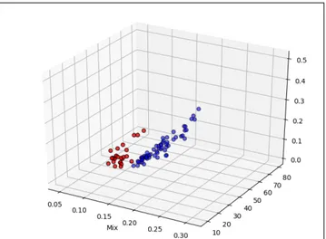
Figure 4. Plotting of Kalz, Harmonic and Closeness cen-tralities for 200 Bach Chorales (blue) and various Beetho-ven pieces (red).

each node, can be correlated with size, however the num-ber of neighbors of a node in the Tonnetz is fixed.

Graph centralities are sufficient for representing the graph obtained from the trajectory and, therefore, we use them for classification. We illustrate this in figure 4 where we plot the Katz, harmonic and closeness centrality for 200 Bach chorales, denoted in blue, and various Beetho-ven pieces, denoted in red (every point represents a piece). A good separation between the two classes is observed.

3. APPLICATION TO CLASSIFICATION In this section, the proposed descriptors are computed from Midi files and used as features in classification me-thods for musical style.

3.1. Descriptors

For the classification experiments we use the va-lues from trajectory descriptors described in section 2 and some other general midi descriptors mainly defined in [28].

For each midi or other file format, we extract the chords using the music21 function chordify [12]. Two trajectories are then built, in different Tonnetze defined by the com-pliance function introduced in section 2.2. We extract the 3 centrality values and 2 clustering coefficients as descri-bed in section 2.3 and the corresponding Tonnetz for each trajectory. Thus, the trajectory descriptor is composed of 12 values.

The general descriptors extract other midi information and general statistics such as the number of instruments in the piece, the type of instruments, an estimated tempo for the piece, the time signature and the number of signature changes. These values are computed using music21 [12] and pretty_midi [29]. These general descriptors and their type are shown in table 1

Descriptor Type Number of Instruments Integer Instruments List of strings Estimated Tempo Integer Time Signatures List of floats Number of Signature changes Integer

Table 1. General Midi Descriptors. 3.2. Classifiers

Two very usual classifiers have been used to evaluate the performance of the descriptors on the data set. The main classifier that obtained repeatedly the best results is the Random Forest Classifier [6]. For the Random Forest Classifier we use a number of 1000 trees. Our experiments have shown that very similar classification results were obtained by varying the number of trees around this value. We also provide results obtained with k-Nearest Neigh-bors (kNN) [11] with k set to 10 neighNeigh-bors, for validation and comparison purposes.

3.3. Music Corpora

Our data set consists of nearly 500 pieces (encoded as midi files) of various composers and styles, namely Stan-dard Jazz, Beethoven, Bach, Mozart, Palestrina, Monte-verdi, Chopin and Schumann (i.e. 8 classes). The data set is well balanced in groups of 60 pieces per compo-ser. Most of the data set is retrieved from music21 corpus [12]. In the corpus we find J.-S. Bach chorales, G. Pales-trina’s vocal works, C. Monteverdi’s madrigals and some works by W. A. Mozart, L. van Beethoven and R. Schu-mann. The rest of the data set was retrieved from several online resources found in [23, 24].

For our data set we used real compositions with no spe-cific requirement or constraint on the midi score quality. In particular, we can use a variety of formats such as xml, mxl, abc, krn and others. All these formats are kinds of symbolic music notation. This way, we approach a more inclusive approach to music score processing and classifi-cation.

3.4. Pre-processing

For the pre-processing of our data, we encode as num-bers the data which are not in numeric form, such as the Tonnetze, the list of instruments, the time signatures, and the list of tempo. We use the label encoder provided by scikit-learn[27]. We also use scikit-learn classifiers, Ran-domForestClassifierand KNeighborsClassifier.

3.5. Experimental Results

The experiments on the data-set with 8 the classes lis-ted above are performed for (i) binary classification (one class against another class), and (ii) multi-class classifica-tion, involving the 8 classes.

The results are evaluated with the F1 score which is

defined as the harmonic mean of the precision and recall :

1st_{Class 2}nd_{Class Random Forest kNN}

Bach Beethoven 1.00 0.97 Bach Chopin 0.97 0.94 Bach Jazz 1.00 0.98 Bach Monteverdi 0.83 0.69 Bach Mozart 1.00 0.98 Bach Palestrina 0.83 0.75 Bach Schumann 0.87 0.92 Table 2. Binary classification : F1-score results with

1000 iterations of Random Forest method, and k-Nearest Neighbors with k = 10. We compared over 60 Bach chorales from music21 corpus versus various works from other composers and style as presented above. We use 70% of the data-set to train the model and the other 30% for testing. Results are for test only, i.e. unseen examples.

F1= 2. precision × recall precision + recall = 2.TP 2.TP + FP + FN (15) where TP are the true positives, FP the false positives and FN the false negatives. The result is a real number in the interval [0, 1] [27].

3.5.1. Binary Classification

For binary classification we use only the trajectory des-criptor. In table 2 we present the F1scores between Bach

chorales and each of the other 7 composers’ styles. The training set contains 70% of the data, and test is performed on the remaining 30% (i.e. not seen before). Therefore, approximately 60 pieces per class were compared. For the Random Forest classifier we produced 1000 decision trees and used information gain to measure each split.

These results show that, for binary classification, the proposed descriptors lead to very good results (F1> 0.8)

with the Random Forest classifier. The results are slightly lower with kNN, as expected. These results demonstrate the relevance of the trajectory descriptors in this simple situation. We can also remark that the lowest scores are achieved between classes where harmony characteristics tend to be most similar. For example, Bach’s chorales tra-jectories received lower scores when compared with Mon-teverdi’s madrigals or Palestrina’s vocal works. We attri-bute this result to the fact that Bach’s chorales have a mo-dal character similar to the one found in renaissance mu-sic.

3.5.2. Multi-class Classification

For multi-class classification we compared the trajec-tory descriptors to the general midi descriptors presented in table 1. Tests have also been carried out using all des-criptors together. Similarly, the Random Forest method was applied with 1000 trees and information gain for the split, and the k-Nearest Neighbors method with k = 10. As in the previous experiment, training was done on 70% of the total samples, and we used the remaining 30% for

Descriptors kNN (k = 10) Random Forest Trajectory 0.49 0.49 MIDI info 0.68 0.76 Combination 0.68 0.82 Table 3. Weighted F1-score for multi-class classification,

with 8 balanced classes labeled by composer, for different descriptors.

testing, arranged in well balanced classes of 60. We ap-plied classification across the 8 classes presented in Sec-tion 3.3 and verified the results using k-fold cross valida-tion with k = 5. Table 3 contains the weighted F1 score

of multi-class classification using different descriptors. One can notice that the trajectory descriptors alone al-ready provide interesting results. Then, when combined with the general descriptors the performance is increased, reaching more than 0.8 for the Random Forest method, and is better (by 6 points) than the results obtained with the general descriptors only.

These results suggest that the combination of des-criptors using the Random Forest Classifier outperforms classification in comparison with [8] with an average of 0.75 across 3 classes, [3] with an average of 0.71 across 6 classes, and [32] with an average of 64.2 across 19 classes. In particular, the approach in [32] uses classifica-tion per composer to which our method outperforms their method on Mozart, Beethoven and Bach classes. However these results should be considered cautiously since the da-tabases used in these approaches differ from the one used in this paper.

In table 4, the confusion matrix as well as the distri-bution of the samples among classes are displayed. The classes are ordered by period (composition dates).

P

alestrina

Monte

v

erdi

Bach Mozart Beetho

v

en

Schumann Chopin Jazz

Palestrina 18 0 0 0 0 0 0 0 Monteverdi 0 17 0 0 0 0 1 0 Bach 1 0 17 0 0 0 1 0 Mozart 0 0 0 10 1 3 5 0 Beethoven 0 0 0 3 20 0 1 0 Schumann 0 0 0 5 1 8 7 0 Chopin 0 0 0 2 1 7 8 0 Jazz 0 0 0 0 0 2 0 16 Table 4. Confusion matrix for multi-class classification with Random Forest. Example reading : 1 Bach piece has been misclassified as Palestrina.

High values (i.e. correct recognition) are obtained on the diagonal. For some styles or composers, almost no er-ror occurs (e.g. Palestrina, Monteverdi, Bach). Moreover most errors (non-zero off-diagonal values) appear close to the diagonal, i.e. between composers of the same per-iod (or close to). From the confusion matrix, we can de-rive that the middling results of the classification come from the classes Mozart, Beethoven, Schumann and

Cho-Descriptors kNN (k = 10) Random Forest Trajectory 0.81 0.84

All descriptors 0.83 0.94

Table 5. F1-score for multi-class classification, with 4

un-balanced classes based on musical style.

Ren. Bar. Class. Jazz Renaissance 35 1 0 0

Baroque 2 15 1 0 Classical 0 0 74 2 Jazz 0 0 3 19 Table 6. Confusion matrix based on musical style with Random Forest.

pin. This observation is crucial as it helps to identify the problem of classification on the harmonic complexity or indifference of a certain compositional period. All compo-sers that appear to yield some classification errors belong to the classical (1730-1820) and romantic period (1800-1850).

This problem is solved when we focus on the clas-sification of style rather than of composer. To this end, the dataset was re-organized into four classes : renais-sance (merging the pieces by Palestrina and Monteverdi), baroque (Bach), classical (Mozart, Beethoven, Schumann and Chopin) and jazz. Results in table 5 show improved performance (even with kNN), and support the claim that works from the same period seem to have similar trajec-tories. As an illustration, we provide the confusion matrix in table 6.

4. CONCLUSION

In this paper we presented novel descriptors for the classification of music style based on symbolic represen-tations and harmonic trajectories. In particular, we exten-ded the definition of a harmonic trajectory first proposed by Bigo [4], and we defined a compliance function that chooses the most appropriate Tonnetz for a piece, in terms of compactness. We have shown that a trajectory can be reduced to 6 values, namely the centralities of the trajec-tory graph, and still be representative of the piece. This was demonstrated by using these trajectory descriptors for the classification of different styles of music. We have ob-tained some promising results in the field of automatic stylistic analysis. In particular in binary classification, we have shown that the trajectory method discriminates up to 100% depending on the style. In comparison with other techniques used in [1, 2, 3, 8, 30, 32] we implemented ge-neral midi descriptors and thus achieved average discrimi-nation up to 82% across 8 classes with the random forest classifier. It should be noted that the approach is agnostic to the type of chords present in the musical piece, and does not depend on a specific dictionary of pre-defined chords. Hence it can be applied to any type of music, including contemporary music.

Future work should concentrate on extending the capa-cities of the trajectory descriptor outside of the pitch-class

barrier by modeling chroma features or even building trajectories in the timbre space [33]. Moreover, we pro-pose working on macro-structure modeling to isolate re-peating structures or rere-peating trajectories that represent a subset of the piece. This process could be achieved using self-similarity matrices and mathematical morpho-logy [15, 22]. Additionally, the approach proposed by Stylerank[13] looks very promising and a future plan will be to combine its features with the trajectory descriptor, as well as chord filtration for result optimization.

Moreover, we propose further testing using multiple descriptors, as well as other classifiers. Last but not least, we reckon on comparing with classification done on ma-jor midi libraries such as the Million Song Dataset and the Lakh Dataset.

5. RÉFÉRENCES

[1] Anan, Y., Hatano, K., Bannai, H., Takeda, M., Sa-toh, K. « Polyphonic Music Classification on Sym-bolic Data Using Dissimilarity Functions », Proceed-ings of the International Society for Music Informa-tion Retrieval Conference, Porto, Portugal, 2012. [2] Armentano, M. G., De Noni, W. A., Cardoso, H. F.

« Genre classification of symbolic pieces of music ». Journal of Intelligent Information Systems48 (2017), p. 579-599.

[3] Basili, R., Serafini, A., Stellato, A. « Classification of musical genre: a machine learning approach », Pro-ceedings of the International Society for Music Infor-mation Retrieval Conference, Barcelone, Espagne, 2004.

[4] Bigo, L. « Représentations symboliques musicales et calcul spatial ». thèse de doctorat, sous la dir. de A. Spicher, M. Andreatta, Université Paris Est, 2013. [5] Boldi, P., Vigna, S. « Axioms for centrality ». Internet

Mathematics10/3-4 (2014), p. 222-262.

[6] Breiman, L. « Random Forests ». Machine Lear-ning45 (2001), p. 5-32.

[7] Carsault, T., Nika, J., Esling, P. « Using musical re-lationships between chord labels in automatic chord extraction tasks. » Proceedings of the International Society for Music Information Retrieval Conference, Paris, 2018.

[8] Cataltepe, Z., Yaslan, Y., Sonmez, A. « Music genre classification using MIDI and audio features ». EURASIP Journal on Advances in Signal Proces-sing2007 (2007).

[9] Catanzaro, M. « Generalized tonnetze ». Journal of Mathematics and Music5/2 (2011), p. 117-139. [10] Conklin, D. « Multiple viewpoint systems for

mu-sic classification ». Journal of New Mumu-sic Re-search42/1 (2013), p. 19-26.

[11] Cover, T., Hart, P. « Nearest neighbor pattern classification ». IEEE Transactions on Information Theory13/1 (1967), p. 21-27.

[12] Cuthbert, M., Ariza, C. « music21: A Toolkit for Computer-Aided Musicology and Symbolic Music Data ». Proceedings of the International Society for Music Information Retrieval Conference, Utrecht, Pays-Bas, 2010.

[13] Ens, J., Pasquier, P. « Quantifying musical style: Ranking symbolic music based on similarity to a style », Proceedings of the International Society for Music Information Retrieval Conference, Delft, Pays-Bas, 2019.

[14] Forte, A. The structure of atonal music. Yale Univer-sity Press, Londres, 1973.

[15] Foote, J. « Visualizing music and audio using self-similarity ». Proceedings of the ACM International Conference on Multimedia, Portland, États-Unis, 1999.

[16] Freeman, L. « Centrality in Networks: I. Conceptual Clarifications ». Social Networks 1/3 (1978-1979), p. 214-239.

[17] Hagberg, A., Schult, D., Swart, P. « Exploring net-work structure, dynamics, and function using Net-workX ». Proceedings of the 7th Python in Science Conference, Pasadena, États-Unis, 2008.

[18] Hillewaere, R., Manderick, B., and Conklin, D. « String quartet classification with monophonic mod-els ». Proceedings of the International Society for Music Information Retrieval Conference, Utrecht, Allemagne, 2010.

[19] Katz, L. « A new status index derived from sociomet-ric analysis ». Psychometrika 18/1 (1953), p. 39-43. [20] Kennedy, M., Bourne, J. The concise Oxford

dic-tionary of music.Oxford University Press, Oxford, 2004.

[21] Lascabettes, P. Homologie Persistante Appliquée à la Reconnaissance de Genres Musicaux, Master 1 Thesis, Ecole Normale Supérieure Paris-Saclay and IRMA/Université de Strasbourg, 2018.

[22] Lascabettes, P. Mathematical Morphology Applied to Music, mémoire de Master, sous la dir. de M. An-dreatta, C. Guichaoua, École Normale Supérieure Paris-Saclay, 2019.

[23] Lucarelli, F. Espace Midi. En ligne. [www. espace-midi.com, accédé le 21 octobre 2020.] [24] McKay, C. MIDI Links. McGill University,

Mont-réal. [www.music.mcgill.ca/~cmckay/ midi.html, accédé le 21 octobre 2020.],

[25] McKay, C., Julie, C., Ichiro F. « JSYMBOLIC 2.2: Extracting Features from Symbolic Music for use in Musicological and MIR Research », Proceedings of the International Society for Music Information Re-trieval Conference, Paris, 2018.

[26] Oldham, S., Fulcher, B., Parkes, L., Fornito, A. « Consistency and differences between centrality measures across distinct classes of networks » PLOS ONE14/7 (2019).

[27] Pedregosa, F. et coll. (+15) « Scikit-learn: Machine Learning in Python » Journal of Machine Learning Research12 (2011), p. 2825-2830.

[28] Raffel, C., Ellis, D. P. W. « Extracting Ground-Truth Information from MIDI Files: A MIDIfesto », Pro-ceedings of the International Society for Music Infor-mation Retrieval Conference, New York, États-Unis, 2016.

[29] Raffel, C., Ellis, D. P. W. « Intuitive analysis, creation and manipulation of MIDI data with pretty_midi », Proceedings of the International Society for Mu-sic Information Retrieval Conference (Late Breaking and Demo Papers), Taipei, Taiwan, 2014.

[30] Ren, Y., Volk, A., Swierstra, W. S., Veltkamp, R. C. « Analysis by classification: A comparative study of annotated and algorithmically extracted patterns in symbolic music data ». Proceedings of the Interna-tional Society for Music Information Retrieval Con-ference, Paris, France, 2019.

[31] Saramäki, J., Kivelä, M., Onnela, J., Kaski, K., Ker-tesz, J. « Generalizations of the clustering coefficient to weighted complex networks ». Physical Review E75/2 (2007), 027105.

[32] Verma, H., Thickstun, J. « Convolutional Composer Classification ». Proceedings of the International So-ciety for Music Information Retrieval Conference, Delft, Pays-Bas, 2019.

[33] Wessel, D. L. « Timbre space as a musical con-trol structure ». Computer Music Journal 3/2 (1979), p. 45-52.