Livrable D6.1 of the PERSEE project : Perceptual Assessment : Definition of the scenarios

(1)

HAL Id: hal-00773183

https://hal.archives-ouvertes.fr/hal-00773183

Submitted on 11 Jan 2013

HAL is a multi-disciplinary open access

archive for the deposit and dissemination of

sci-entific research documents, whether they are

pub-L’archive ouverte pluridisciplinaire HAL, est

destinée au dépôt et à la diffusion de documents

scientifiques de niveau recherche, publiés ou non,

Livrable D6.1 of the PERSEE project : Perceptual

Assessment : Definition of the scenarios

Junle Wang, Josselin Gautier, Emilie Bosc, Jing Li, Vincent Ricordel

To cite this version:

Junle Wang, Josselin Gautier, Emilie Bosc, Jing Li, Vincent Ricordel. Livrable D6.1 of the PERSEE

project : Perceptual Assessment : Definition of the scenarios. 2011, pp.62. �hal-00773183�

(2)

Projet PERSEE

´ SchÈmas Perceptuels et Codage vidÈo 2D et 3D

a

n◦ ANR-09-BLAN-0170 Livrable D6.1 15/10/2011

Perceptual Assessment :

Definition of the scenarios

Junle WANG IRCCyN Josselin GAUTIER IRISA

Emilie BOSC INSA Jing LI IRCCyN Vincent RICORDEL IRCCyN

(3)

Contents 2

1 Introduction

In this report we describe contributions for the task 6 within the PERSEE project. The target of this task is to carry on the perceptual and subjective performance assessment of the tools developed for the project.

Here we present the definition of the scenarios of the experimental tests that have been done in link with the perceptual models of the task 1 (these models are described in the deliverable D1.2 entitled "Perceptual Modelling: Definition of the models"). We present also the tests that have been done to assess the subjective quality of synthesized contents.

The document is organized as follows:

• Section 1 is about the test to assess the impact of the blur on the depth percep-tion;

• Section 2 presents the test to assess the depth bias;

• Section 3 presents the test to assess the subjective quality of synthesized contents (coded or not);

• Section 4 presents the test to assess the visual discomfort induced by moving stimulus.

2 Test to assess the impact of the blur on the depth

perception

When 3D images are shown on a planar stereoscopic display, binocular disparity be-comes a pre-eminent depth cue. But it induces simultaneously the conflict between accommodation and vergence, which is often considered as a main reason for visual discomfort. If we limit this visual discomfort by decreasing the disparity, the apparent depth also decreases. This psychophysical experiment was designed to quantitatively evaluate the influence of a monocular depth cue, blur, on the apparent depth of stereo-scopic scenes.

We propose to decrease the (binocular) disparity of 3D presentations, and to rein-force (monocular) cues to compensate the loss of perceived depth and keep an unaltered apparent depth. We conducted a subjective experiment using a two-alternative forced choice task. Observers were required to identify the larger perceived depth in a pair of 3D images with/without blur. By fitting the result to a psychometric function, we obtained points of subjective equality in terms of disparity, from which we could compute the increase of perceived depth caused by blur.

(6)

2.1 Subjects

Thirty-five subjects participated in the experiment. Twelve subjects are male, twenty-three are female. The subjects did not know about the purpose of the experiment. Subjects ranged in age from 17 to 40 years. All had either normal or corrected-to-normal visual acuity. They were tested for visual acuity using a Snellen Chart, for depth acuity using a Randot Stereo Test and for color vision using Ishihara plates.All the subjects were compensated and were naive to the purpose of the experiment.

2.2 Apparatus

One of the limitations of previous studies was the apparatus used. CRT monitors were used and this type of displays has some drawbacks: (1)the surface containing stimuli was slightly curved, (2) the stimuli’s virtual distance was affected by refraction due to the front glass plate, and (3) the screen was usually not large enough to cover a favorable field-of-view.

In our study, state-of-the-art stereoscopic display was used. Stimuli were displayed on a Samsung 22.5-inch LCD screen (figure 1), which had a resolution of 1680 * 1050 pixels, and the refresh rate was 120 Hz. Each screen pixel subtended 65.32 arcsec at a 90 cm viewing distance. The display yielded a maximum luminance of about 50 cd/m2 _{when watched through the activated shutter glasses. Stimuli were viewed}

binocularly through the Nvidia active shutter glasses (Nvidia 3D Vision kit) at a dis-tance of approximately 90 cm. The peripheral environment luminance was adjusted to about 44 cd/m2_{. When seen through the eye-glasses, this value corresponded to}

about 7.5 cd/m2 _{and thus to 15% of the screen’s maximum brightness as specified by}

ITU-R BT.500.

(a) (b)

Figure 1: Apparatus. (a) Samsung SyncMaster 2233 monitor; (b) Nvidia 3D vision kit.

(7)

2.3 Stimuli

Each stimulus consisted of one single object in the foreground and a background. A 400 * 400 pixels butterfly image was used as the foreground object. This stimulus was easy to accommodate because it was spatially complex and therefore contained a wide range of spatial frequencies from low to high. The butterfly was shown with a horizontal offset between the left and the right view in order to create a disparity cue. The magnitude and direction of this offset varied to supply a variety of near or far disparity. At the 90 cm viewing distance, the background plane subtended 29.8 * 18.9 arcdeg, and the foreground object subtended 7.2 arcdeg. The background plane was a photo of a flowerbed. The background contained a great amount of textures, contained no distinct region of interest distracting the observers, and looked natural. When re-quired, the background was spatially blurred by applying a Gaussian blur kernel with a 5-pixel radius. This amount of blur equals to the blur created by supposing that the focused object (foreground) and the defocused object (background) are at a distance of 13.7 cm in front of the screen and 19.8 cm behind the screen respectively, both of which are the limitations of the comfortable viewing zone derived from the 90 cm view-ing distance. Note that all the blurred background were with the same amount of blur.

2.4 Design and procedure

In each trial, a pair of stimuli were shown to the subjects. One stimulus contained a blurred background (BB) and a sharp foreground object, while the other stimulus contained a sharp background (SB) and also a sharp foreground object (as shown in figure 2). The backgrounds of both stimuli were positioned at the same depth. Two parameters of the stimuli were varied: the absolute position (Da) of the background

plane and the relative distance (Dr) of the foreground object to the background. The

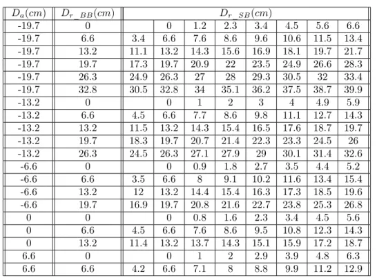
selection of absolute distance ranged from -19.7 cm to 6.6 cm in steps of 6.6 cm (neg-ative values denote the positions behind the screen plane, and positive values denote the positions in front of the screen plane). The relative distance ranged from 0 cm to approximately 33 cm. All the positions of both background and foreground objects are selected considering the limitations of the comfortable viewing zone[13]. There are thus twenty combinations of absolute position and relative distance in total for the BB-stimuli.

Once the absolute position and the relative distance were selected for each BB-stimulus, then we paired the BB-stimulus with a set of 7 or 8 SB stimuli which are with relative distances ranging from 4 cm less than the BB stimulus to 8 cm larger than the reference stimulus. These steps were chosen considering both the depth ren-dering ability of the screen and the depth perception ability of the observers. One trial contains one BB-stimulus and one SB-stimulus. We had 155 trials in the experiment. This setup is shown in Figure 3, and the parameters are shown in Table 1.

(8)

(a) The left view of a Sharp-Background (SB) stimuli

(b) The left view of a Blur-Background (BB) stimuli

Figure 2: Example Stimuli

butterfly is located, the red plane represents the depth plane in which the background is located. We named the distance between background plane and the screen as Absolute Position (Da), while the interval between the foreground plane and the background

plane as the Relative Distance (Dr). Both these two distances were free parameters

of the design of stimuli. The variation range of these two planes always stayed in the comfortable viewing zone. The first figure shows the BB-stimulus case, while the second shows the SB-stimulus case. Each BB-stimulus is paired with one of 7 or 8 SB-stimuli to create one trial. The selection of the parameters Da and Dr for both

(9)

(a)

(b)

Figure 3: Schematic diagram of the experiment setup

The subjective experiment was conducted using a two-alternative forced choice task. For each trial, one of the 155 conditions was chosen randomly and a pair of stimuli were displayed. Observers were asked to look at the butterfly and then determine in the trial whether the BB stimulus contained a larger depth interval between the

(10)

Test to assess the impact of the blur on the depth perception 9 Da(cm) Dr_BB(cm) Dr_SB(cm) -19.7 0 0 1.2 2.3 3.4 4.5 5.6 6.6 -19.7 6.6 3.4 6.6 7.6 8.6 9.6 10.6 11.5 13.4 -19.7 13.2 11.1 13.2 14.3 15.6 16.9 18.1 19.7 21.7 -19.7 19.7 17.3 19.7 20.9 22 23.5 24.9 26.6 28.3 -19.7 26.3 24.9 26.3 27 28 29.3 30.5 32 33.4 -19.7 32.8 30.5 32.8 34 35.1 36.2 37.5 38.7 39.9 -13.2 0 0 1 2 3 4 4.9 5.9 -13.2 6.6 4.5 6.6 7.7 8.6 9.8 11.1 12.7 14.3 -13.2 13.2 11.5 13.2 14.3 15.4 16.5 17.6 18.7 19.7 -13.2 19.7 18.3 19.7 20.7 21.4 22.3 23.3 24.5 26 -13.2 26.3 24.5 26.3 27.1 27.9 29 30.1 31.4 32.6 -6.6 0 0 0.9 1.8 2.7 3.5 4.4 5.2 -6.6 6.6 3.5 6.6 8 9.1 10.2 11.6 13.4 15.4 -6.6 13.2 12 13.2 14.4 15.4 16.3 17.3 18.5 19.6 -6.6 19.7 16.9 19.7 20.8 21.6 22.7 23.8 25.3 26.8 0 0 0 0.8 1.6 2.3 3.4 4.5 5.6 0 6.6 4.5 6.6 7.6 8.6 9.5 10.8 12.3 14.3 0 13.2 11.4 13.2 13.7 14.3 15.1 15.9 17.2 18.7 6.6 0 0 1 2 2.9 3.9 4.8 6.3 6.6 6.6 4.2 6.6 7.1 8 8.8 9.9 11.2 12.9

Table 1: The selection of parameters Da and Dr for both BB-stimuli and SB-stimuli.

Note that there are only 7 possible selections for the Dr_BB, because putting

the foreground behind the background will cause trouble of fusion.

butterfly and the background than the SB stimulus. As a two monitor screen setup was technically not possible, observers were able to control the displaying of stimuli by means of a key press to switch from one stimulus to the other. When the observer switched between the stimuli, a 700 ms grey interval was shown in order to avoid memorization by the observers of the "exact" positions of the foregrounds. For each trial, the total observation time and the number of switches were not limited.

2.5 Result and data analysis

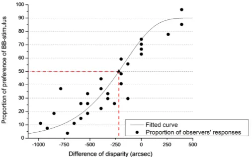
For each condition, some observers considered the BB-stimulus as having a larger depth interval (between the foreground and the background), while the other observers chose the SB-stimulus. We measure the proportion of ’BB-stimulus contains a larger depth interval’ responses, and plot the data as a function of the disparity difference between the Dr in the BB-stimulus (Dr_BB) and the Dr in the SB-stimulus (Dr_SB). The

cumulative Weibull function was used as the psychometric function. The disparity difference corresponding to the 50% point can be considered as the Point of Subjective Equality (PSE). When measuring the disparity difference at that point, the increase

(11)

of perceived depth is obtained. In total, by filtering out the data of 7 observers who made decisions in the test quite differently from other observers, 28 observations of each conditions were included in the computation. An example pattern of response and the fitted psychometric function is shown in Figure 4.

Figure 4: An example pattern of the proportion of observers’ responses and the fitted psychometric function. In this trial, we consider Dr_BB = 6.6 cm and Da

= -19.7 cm, -13.2 cm, -6.6 cm, 0 cm, 6.6 cm. An equal apparent depth is reached at -220 arcsec

(12)

Test to assess the depth bias 11

3 Test to assess the depth bias

In the studies of 2D visual attention, eye-tracking data shows a so-called "center-bias", which means that fixations are biased towards the center of 2D still images. However, in the stereoscopic visual attention, depth is another feature having great influence on guiding eye movements. Relative little is known about the impact of depth.

We conducted a binocular eye-tracking experiment by showing synthetic stimuli on a stereoscopic display. Observers were required to do a free-viewing task through ac-tive shutter glasses. Gaze positions of both eyes were recorded for obtaining the depth of fixation. Stimuli were well designed in order to let the center-bias and depth-bias affect eye movements individually. Results showed that the number of fixations varies as a function of depth planes.

3.1 Stimuli

Synthetic stereoscopic stimuli were used for this experiment. The stimuli consisted in the presentation of scenes in which a background and some similar objects were delib-erately displayed at different depth positions. We generated the depth by horizontally shifting the objects to simulate the binocular disparity. This was also the only depth cue we took advantage of in this experiment.

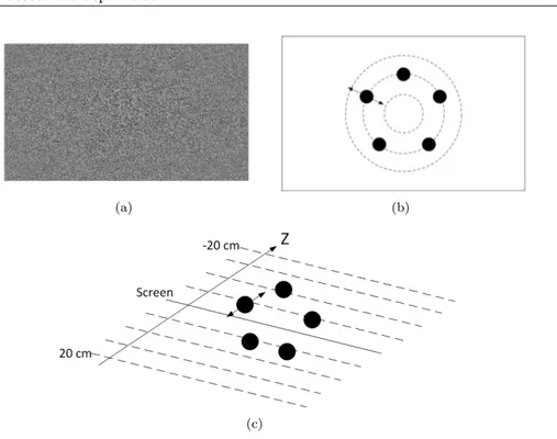
The background was a flat image consisting in white noise (figure 5 (a)), which was placed at a depth value of -20 cm (20 cm beyond the screen plane). In each scene, the objects consisted in a set of black disks of the same diameter S. They were displayed at different depth values randomly chosen among {-20, -15, -10, -5, 0, 5, 10, 15, 20} cm. Though the objects were placed at different depths (figure 5 (b)), the positions of projection of the objects on the screen plane uniformly laid on a circle centered on the screen center (figure 5 (c)). Thus, we assume that no "center-bias" was introduced in the observation.

Three parameters were varying from one scene to another: 1, the number of objects, N ∈ {5, 6, 7, 8, 9}; 2, the radius R of the circle on which the objects were projected on the screen plane, R ∈ {200, 250, 300} pixels; 3, the size of the objects, which was represented by the diameter of the disk S varying from πR

N√2 to 2πR

N√2. The range is

selected in order to avoid any overlap of the objects. Derived from the combinations of this set of parameters, 118 scenes were presented to each observer. Each scene was presented for 3 seconds. Figure 6 gives the examples of the scenes.

There were three advantages of using this kind of synthetic stereoscopic stimuli to investigate the depth-bias:

• Firstly, compared to natural content, synthesis stimuli were easier to control. We could precisely allocate the position and depth of every object in the scene. This

(13)

(a) (b)

(c)

Figure 5: Composition of the stimuli. (a)The background of the stimuli. Only white-noise is contained in the background, which is positioned behind all the stimuli at -20 cm depth plane. (b)Positions of the objects’ projections on the screen plane. All the projections laid uniformly on a circle center at the screen center.(c)Allocation of objects in the depth range from -20 cm to 20 cm.

accurate control of the scene could enabled us a better quantitative analysis of eyes movement.

• Secondly, even in 3D viewing, human’s eye movements were affected by many bottom-up 2D visual features of the stimuli, such as color, intensity, object’s size, and the center-bias. These factors could contaminate our evaluation of depth’s influence on visual attention. In our experiment, for each condition, all the objects were with the constant shape, constant size, and constant distance to the center of the screen. This set up let the stimuli get rid of as many bottom-up visual attention features as possible. The white noise background and the simple allocation of objects could also avoid the as much as possible the influence of top-down mechanism in visual attention.

• Third, the complexity of scenes presented to the observers was low, which enable a shorter observation duration. The duration of eye-tracking experiments for natural content images was usually 10 seconds or more. Compared to that, the

(14)

(a) (b) (c)

(d) (e)

Figure 6: Examples of stimuli with different number of objects used in the eye-tracking experiment.

observation duration time in our experiment was relatively short (3 seconds for each condition), nevertheless, it was still long enough for participants to explore the scene as they want and subconsciously position their fixations of the objects. Hence, using these simple stimuli allowed experimenters to collect more data, as well as learn the evolution of depth-bias over time.

3.2 Participants

Twenty-seven subjects participated in the experiment. 12 subjects are male, 15 are female. The subjects ranged in age from 18 to 44 years. The mean age of the subjects was 22.8 years old. All the subjects had either normal or corrected-to-normal visual acuity, which was verified by three pretests before the start of eye-tracking experiment. Monoyer chart was used to check the acuity (subject must get the result higher than 9/10); Ishihara test was used to check the color vision (subject should be without any color troubles); and Randot stereo test was used to check the 3D acuity (subject should get the result higher than 7/10). Among the subjects, 23 of them were students, 3 were university staffs, and 1 software developer. All of them were naive to the purpose of the experiment, and were compensated for the participation of the experiment.

3.3 Apparatus and procedures

Stimuli were displayed on a 26-inch (552 mm * 323 mm) Panasonic BT-3DL2550 LCD screen (figure 7 (a)), which had resolution of 1920 * 1200 pixels, and the refresh rate was 60 Hz. Each screen pixel subtended 61.99 arcsec at a 93 cm viewing distance. The maximum luminance of the display was 180 cd/m2, which yielded a maximum luminance of about 60 cd/m2 when watched through the glasses. Observers viewed the

(15)

(a) (b)

(c)

Figure 7: (a)The 26-inch Panasonic BT-3DL2550 LCD screen used in the experiment. (b)SMI

stereoscopic stimuli through a pair of passive polarized glasses at a distance of 93cm. The environment luminance was adjusted according to each observer, in order to let the pupil has an appropriate size for eye-tracking. SMI RED 500 remote eye-tracker was used to record the eye movements (figure 7 (b)).

The viewing distance corresponds to a 33.06 * 18.92 degrees field of view of the background of the stimuli, all the objects were displayed in an area within 10.32*5.91 degrees. A chin-rest was used to stabilize observer’s head (figure 7 (c)), and the ob-servers were instructed to "view anywhere on the screen as they want".

(16)

center point was showed for 500 ms at the screen center with zero disparity. A nine-point calibration was performed at the beginning of the experiment, and repeated every twenty scenes. The quality of calibration was verified by the experimenter on another monitor. Participants could require for a rest before every calibration started.

3.4 Post processing of eye tracking data

The recorded eye movements were first processed by the Begaze software provided by SMI to identify fixations and filter out saccades. Each fixation was then decided if it was located on one of the objects or not. A fixation was considered to be located on an object if it was positioned on the object or within a surrounding area (10% larger than the object’s size). Otherwise, the fixation was considered to be on the background. Therefore, the depth information of each fixation could be obtained. Note that only the ’on target’ fixations (the fixations located on a object) were considered in the fol-lowing analysis.

(17)

Existence of a depth bias on natural images 16

4 Existence of a depth bias on natural images

4.1 Experimental condition of occulometric database

The eye tracking dataset provided by Jansen et al. is used in this section [27]. We briefly remind the experimental conditions, i.e. materials and methods to construct this database in 2D and 3D conditions. Stereoscopic images were acquired with a stereo rig composed of two digital cameras. In addition, a 3D laser scanner was used to measure the depth information of these pairs of images. By projecting the acquired depth onto the images and finding the stereo correspondence, disparity maps were then generated. The detailed information relative to stereoscopic and depth acquisition can be found in [32]. The acquisition dataset is composed of 28 stereo images of forest, undistorted, cropped to 1280x1024 pixels, rectified and converted to grayscale. A set of six stimuli was then generated from these image pairs with disparity information: 2D and 3D versions of natural, pink noise and white noise images. Our study focuses only on 2D and 3D version of natural images of forest. In 2D condition two copies of the left images were displayed on an auto stereoscopic display. In 3D condition the left and right image pair was displayed stereoscopically, introducing a binocular disparity to the 2D stimuli.

The 28 stimulus sets were split-up into 3 training, 1 position calibration and 24 main experiments sets. The training stimuli were necessary to allow the participant to become familiar with the 3D display and the stimulus types. The natural 3D image of the position calibration set was used as reference image for the participants to check their 3D percept.(cited from Jansen et al.[27])

A 2 view auto stereoscopic 18.1” display (C-s 3D display from SeeReal technologies, Dresden, Germany) was used for stimuli presentation. The main advantage of such display is that it doesn’t require special eyeglasses. A tracking system adjusts the two view display to the user position. A beam splitter in front of the LCD panel projects all odd columns to a dedicated angle of view, and all even ones to another. Then, through the tracking system, it ensures the left eye perceives always the odd columns and the right eye the even columns whatever the viewing position. A “3D” effect introducing binocular disparity is then provided by presenting a stereo image pair interlaced vertically. In 2D condition, two identical left images are vertically interlaced. The experiment involved 14 participants. Experiment was split into two sessions, one session comprising a training followed by two presentations separated by a short break. The task involved during presentation is of importance in regards to the literature on visual attention experiments. Here, instructions were given to the subjects to study carefully the images over the whole presentation time of 20s. They were also requested to press a button once they could perceive two depth layers in the image. One subject misunderstood the task and pressed the button in all images. His data were excluded from the analysis. Finally, participants were asked to fixate a cross marker with zero disparity, i.e. on the screen plane, before each stimulus presentation. The fixation corresponding to the prefixation marker was discarded, as each observer started to look at a center fixation cross before the stimuli onset and this would biased the fixation to this region at the first fixation. An “Eyelink II” head-mounted

(18)

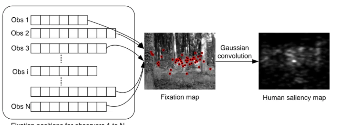
Fixation positions for observers 1 to N Obs 1 Obs 2 Obs 3 Obs i Gaussian convolution Obs N

Fixation map Human saliency map

Figure 8: Illustration of the human saliency map computation from N observers

occulometer (SR Research, Osgoode, Ontario, Canada) recorded the eye movements. The eye position was tracked on both eyes, but only the left eye data were recorded; as the stimulus on this left eye was the same in 2D and 3D condition (the left image), the binocular disparity factor was isolated and observable. Observers were placed at 60 cm from the screen. The stimuli presented subtended 34.1◦ horizontally and 25.9◦ vertically. Data with an angle less than 3.75◦ to the monitor frame were cropped. In the following sections, either the spatial coordinates of visual fixations or ground-truth i.e. human saliency map is used. The human saliency map is obtained by convolving a 2D fixation map with a 2D Gaussian with full-width at half-maximum (FWHM) of one degree. This process is illustrated in Figure 8

4.2 Behavioral and computational studies

Jansen et al. [27] gave evidence that the introduction of disparity altered the basic properties of eye movement such as rate of fixation, saccade length, saccade dynamics, and fixation duration. They also showed that the presence of disparity influences the overt visual attention especially during the first seconds of viewing. Observers tend to look at closer locations at the beginning of viewing. We go further by examining four points: first we examine whether the disparity impacts the spatial locations of salient areas. Second, we investigate the mean distance between fixations and screen center, i.e. the center bias in 2D and 3D condition. The same examination is done over the depth bias in both viewing conditions. The last question is related to the disparity influence on the of state-of-the-art models performance of bottom-up visual attention.

4.2.1 Do salient areas depend on the presence of binocular disparity?

The area under the Receiver Operating Characteristic (ROC) curve is used to quantify the degree of similarity between 2D and 3D human saliency maps. The AUC (Area Under Curve) measure is non-parametric and is bounded by 1 and 0.5. The upper

(19)

Figure 9: Boxplot of the AUC values between 2D and 3D human (experimental) saliency maps as a function of the number of fixations (the top 20% 2D salient areas are kept).

bound indicates a perfect discrimination whereas the lower bound indicates that the discrimination (or the classification) is at the chance level. The thresholded 3D saliency map is then compared to the 2D saliency map. For the 2D saliency maps taken as reference, the threshold is set in order to keep 20% of the salient areas. For 3D saliency maps, the threshold varies linearly in the range of 0 to 255. Figure 9 shows AUC values in function of the fixation rank. Over the whole viewing time (called “All” on the right-hand side of Figure 9), the AUC value is high. The median value is equal to 0.81 0.008 (mean±SEM). When analyzing only the first fixations, the similarity degree is the lowest. For instance, the similarity increases from 0.68 to 0.81 in a significant manner (F(1, 23)=1.8,p<0.08, paired t(23)=13.73, p0.01). Results suggest that the disparity influences the overt visual attention just after the stimuli onset. This influence significantly lasts up to the first 30 fixations (F(1, 23)=0.99,p<0.49), paired t(23)=4.081.64, p<0.0001).

Although the method used to quantify the influence of stereo disparity on the allo-cation of attention is different from the work of Jansen et al. [27], we draw the same conclusion. The presence of disparity on still pictures has a time-dependent effect on our gaze. During the first seconds of viewing (enclosing the first 30 fixations), there is a significant difference between the 2D and 3D saliency maps.

(20)

4.2.2 Center bias for 2D and 3D pictures

Previous studies have shown that observers tend to look more at the central regions of a scene displayed on a screen than at the peripheral regions. This tendency might be explained by a number of reasons (see for instance [49]). Recently, Bindemann [6] demonstrated that the center bias is partly due to an experimental artifact stemming from the onscreen presentation of visual scenes. He also showed that this tendency was difficult to remove in a laboratory setting. Does this central bias still exist when viewing 3D scenes? This is the question we address in this section.

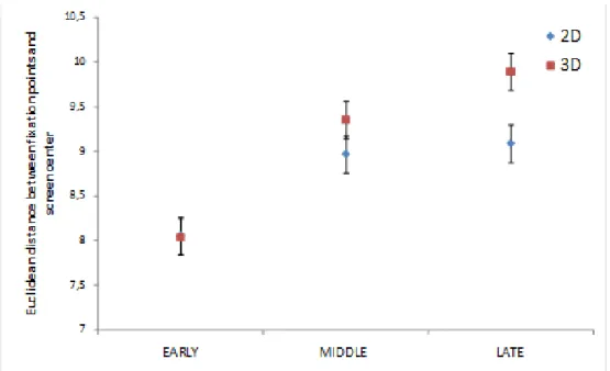
Figure 10: Average Euclidean distance between the screen center and fixation points. The error bars correspond to SEM (Standard Error of the Mean).

When analyzing the fixation distribution, the central bias is observed for both 2D and 3D conditions. The highest values of the distribution are clustered around the center of the screen (see Figure 11 and Figure 12). This bias is more pronounced just after the stimuli onset. To quantify these observations further, a 2x3 ANOVA with the factors 2D-3D (stereoscopy) and three slots of viewing times (called early, middle and late) is applied to the Euclidean distance of the visual fixations to the center of the screen. Each period is composed of ten fixations: early period consists of the first ten fixations, middle the next ten and the late period is composed of the ten fixations occurring after the middle period. A 2x3 ANOVA shows a main effect of the stereoscopy factor F(1, 6714) = 260.44 p<0.001, a main effect of time F(2, 6714) = 143.01 p<0.001 and an interaction between both F(2, 6714) = 87.16 p<0.001. First the influence of viewing time on the center bias is an already known factor. Just after

(21)

the stimuli onset, the center bias is more pronounced than after several seconds of viewing. Second there is a significant difference of the central tendency between 2D and 3D conditions and that for the three considered time periods.

Bonferroni t-tests however showed that the central tendency is not statistically sig-nificant (2D/3D) for the early periods as illustrated by Figure 3. For the middle and late periods, there is a significant difference in the central bias (p<0.0001 and p«0.001, respectively). The median fixation durations were 272, 272 and 276ms in 2D condition and 276, 272 and 280ms in 3D condition for early, middle and late period respectively.

Figure 11: (a) and (b) are the distributions of fixations for 2D and 3D condition, respectively. (c) and (d) represent the horizontal and vertical cross sections through the distribution shown in (a) and (b). All the visual fixations are used to compute the distribution.

(22)

Figure 12: (a) and (b) are the distributions of fixations for 2D and 3D condition, respectively. (c) and (d) represent the horizontal and vertical cross sections through the distribution shown in (a) and (b). All the visual fixations are used to compute the distribution.

(23)

4.2.3 Depth bias: do we look first at closer locations?

In [27], a depth bias was found out suggesting that observers tend to look more to closer areas just after the stimulus onset than to further areas. A similar investigation is conducted here but with a different approach. Figure 13 illustrates a disparity map: the lowest values represent the closest areas whereas the furthest areas are represented by the highest ones. Importantly, the disparity maps are not normalized and are linearly dependent on the acquired depth.

Figure 13: Original picture (a) and its disparity map (black areas stand for the closest areas whereas the bright areas indicate the farthest ones).

We measured the mean disparity for each fixation point in both conditions (2D and 3D). A neighborhood of one degree of visual angle centered on fixation points is taken in order to account for the fovea size. A 2x3 ANOVA with the factors 2D-3D (stereoscopy) and three slots of viewing times (called early, middle and late) is performed to test the influence of the disparity on the gaze allocation. First the stere-oscopy factor is significant F(1, 6714) = 8.8 p<0.003. The factor time is not significant F(2,6714)=0.27 p<0.76. Finally, we observed a significant interaction between both factors F(2,6714)=4.16 p<0.05. Bonferroni t-tests showed that the disparity has an influence at the beginning of the viewing (called early), (p<0.0001). There is no dif-ference between 2D and 3D for the two others time periods, as illustrated by Figure 14.

(24)

Test to assess the subjective quality of 2D and 3D synthesized contents (with or

without compression) 23

Figure 14: Mean disparity (in pixels) in function of the viewing time (early, middle and late). The error bars correspond to SEM (Standard Error of the Mean).

4.2.4 Conclusion

In this behavioral section based on occulometric experiments, we investigated whether the binocular disparity significantly impacts our gaze on still images. It is, especially on the first fixations. This depth cue induced by the stereoscopic condition indeed impacts our gaze strategy: in stereo condition and for the first fixations, we tend to look more at closer locations. These confirm the work of Jansen et al. [27], and support the existence of a depth bias.

5 Test to assess the subjective quality of 2D and 3D

synthesized contents (with or without compression)

Depth-Image-Based-Rendering algorithms are used for virtual view generation, which is required in both applications. This process induces new types of artifacts. Con-sequently it impacts on the quality, which has to be identified considering various contexts of use. While many efforts have been dedicated to visual quality assessment in the last twenty years, some issues still remain unsolved in the context of 3DTV. Actually, DIBR is bringing new challenges from the visual quality perspectives mainly because it deals with geometric distortions, which have been barely addressed so far.

Virtual views synthesized either from decoded and distorted data or from original data, need to be assessed. The best assessment tool remains the human judgment as long as the right protocol is used. Subjective quality assessment is still delicate while

(25)

addressing new type of conditions because one has to define the optimal way to get reliable data. Tests are time-consuming and consequently one should draw big lines on how to conduct such experiment to save time and observers. Since DIBR is introducing new conditions, the right protocol to assess the visual quality with observers is still an open question. The adequate protocol might vary according to the purpose (impact of compression, DIBR techniques comparison ). Since subjective quality assessment tests are time-consuming, objective metrics have been developed and are extensively used. They are meant to predict human judgment and their reliability is based on their correlation to subjective assessment results. As, the way to conduct the subjective quality assessment protocols is already questionable, reliability of objective quality metrics among existing ones that could be useful in DIBR context, should be tested in the new conditions.

Yet, trustworthy working groups base partially their future specifications, concerning new strategies for 3D video, on the outcome of objective metrics. Considering the test conditions may rely on usual subjective and objective protocols (because of their availability), the outcome of wrong choices could result to a poor quality of experience for users. Then, new tests should be carried on to determine the reliability of subjective and objective quality assessment tools in order to exploit their results for the best.

In this study, we propose to answer two questions: First, how adapted are the used subjective assessment protocols in the case of DIBR-based rendered virtual views? Second, is there a correlation between commonly used 2D video metrics scores and subjective scores when evaluating the quality of DIBR-based rendered virtual views? Indeed, we first address the 2D conditions because it is a first step that should be stud-ied, before including parameters such as 3D vision, that are not completely understood at the moment.

5.1 New artifacts related to DIBR

As explained in the introduction, DIBR is brings new types of artifact, different from those commonly encountered in video compression: most video coding standards rely on DCT, and the resulting artifacts are specific (some of them are described in [61]). Artifacts brought by DIBR are mainly geometric distortions. They are related to two causes: the accuracy of incoming data values (e.g. depth estimation accuracy) and the synthesis process strategies. Note that they are also different from stereoscopic impairments (such as cardboard effect, crosstalk, etc. as described in [33]), which occur in stereoscopic conditions (fusion of left and right views in human visual system). Synthesis process strategies mainly aimed at dealing with the critical problem in DIBR, namely the disocclusion: when generating a new viewpoint, areas that were not visible in the reference viewpoint, become visible in the new point. They are discovered. There is no available color in-formation to fill in these areas, which leads to geometric distortions. Extrapolation techniques are meant to fill the disoccluded regions.

In this section, typical DIBR artifacts are described. In most of the cases, these artifacts are located around large depth discontinuities, but they are more perceptible in case of high texture contrast between background and foreground.

(26)

chosen extrapolation method (if the method chooses to assign the background values to the missing areas, object may be resized), or on the encoding method (blocking artifacts in depth data result in object shifting in synthesis). Figure 15 depicts this type of artifact.

(a) Original frame (b) Synthesized frame

Figure 15: Shifting/Resizing artifacts

Blurry regions: This may be due to the inpainting method used to fill the disoc-ccluded areas. It is obvious around the background/foreground transitions. These remarks are confirmed on Figure 16 around the disoccluded areas.

(a) Original frame (b) Synthesized frame

Figure 16: Blurring artifacts (Book Arrival)

Texture synthesis: inpainting methods can fail in filling complex textured areas. To overcome these limitations, a hole filling approach based on patch-based texture

(27)

synthesis is proposed in [35].

Flickering: when errors occur randomly in depth data along the sequence, pixels are wrongly projected: some pixels suffer slight changes of depth, which appears as flickers in the resulting synthesized pixels. To avoid this methods such as [30] propose to acquire background knowledge along the sequence and to conse-quently improve the synthesis process.

Tiny distortions: in synthesized sequences, a large number of tiny geometric distor-tions and illumination differences are temporally constant and perceptually invisible. However, pixel-based metrics may penalize these distorted zones.

When encoding either depth data or color sequences before performing the synthe-sis, compression-related artifacts are combined with synthesis artifacts. Artifacts from data compression are generally scattered within the whole image, while artifacts in-herent to the synthesis process are mainly located around the disoccluded areas. The combination of both type of distortion, depending on the compression method, rela-tively affects the synthesized view. Indeed, most of the used compression methods are 2D video codecs inspired, and are thus optimized for human perception of color. As a result, artifacts occurring especially in depth data induce severe distortions in the synthesized views. In the following, a few examples of such distortions are presented. Blocking artifacts: this occurs when the compression method induces blocking arti-facts in depth data. In the synthesized views, whole blocks of color image seem to be translated. Figure 17 illustrates the distortion.

(a) Original depth frame (up) and color original frame (bottom)

(b) Decoded depth frame (up) and re-sulting synthesized frame (bottom)

Figure 17: Blocking artifacts from depth data compression result in distorted synthe-sized views (Breakdancers).

(28)

Ringing artifacts: when ringing artifacts occur in depth data around strong discon-tinuities, objects edges appear distorted in the synthesized view. Figure 18 depicts this artifact.

(a) Original depth frame (up) and original color frame (bottom)

(b) Distorted depth frame (up) and resulting synthesized frame (bottom)

Figure 18: Ringing artifacts in depth data lead to distortions in the synthesized views.

5.2 Subjective quality assessment methodologies

In the absence of any better 3D-adapted subjective quality assessment methodologies, the evaluation of synthesized views is mostly obtained through 2D validated protocols. Different methods were developed by the ITU-R and ITU-T. The appropriate method is selected, according to one objective. Indeed the methods differ depending on the type of distortion and on the evaluation. In the case of synthesized views evaluation, one should choose the adequate subjective method. This section introduces two reliable 2D subjective quality assessment methodologies, based on the proposed classification of subjective test protocols described in [5], and on the methods described in [9]. Then requirements for 3D-adapted subjective quality assessment protocols are presented.

Absolute categorical rating with Hidden Reference Removal (ACR-HR) methodology [4] consists in presenting test objects (i.e. images or sequences) to ob-servers. The objects are presented one at a time and in a random order, to the observers. Observers score the test item according to a discrete category rating scale. From the scores obtained, a differential score (DMOS for Differential Mean Opinion Score) is computed between the mean opinion scores (MOS) of each test object and its associated hidden reference. The quality scale recommended by ITU-R is depicted

(29)

Test to assess the subjective quality of 2D and 3D synthesized contents (with or without compression) 28 5 Excellent 4 Good 3 Fair 2 Poor 1 Bad

Table 2: Comparison scale for ACR-HR

in Table 2. ACR-HR methodology is a single stimulus method.

The results of an ACR-HR test are obtained by averaging observers’ opinion scores for each stimulus, in other words, by computing mean opinion scores (MOS). ACR-HR requires many observers to minimize the contextual effects (previously presented stim-uli influence the observer opinion, i.e. presentation order influences opinion ratings). Accuracy increases with the number of participants.

Paired comparisons (PC) methodology [4] is an assessment protocol in which stimuli are presented by pairs to the observers: it is a double-stimulus method. The latter select the one out of the pair that best satisfies the specified judgment criterion, i.e. image quality. The results of a paired comparisons test are recorded in a ma-trix: each element corresponds to the frequencies a stimulus is preferred over another stimulus. These data are then converted to scale values using Thurstone-Mosteller’s or Bradley-Terry’s model [22]. It leads to a hypothetical perceptual continuum. The presented experiments follow Thurstone-Mosteller’s model where naive observers were asked to choose the preferred item from one pair. Although the method is known to be highly accurate, it is time consuming.

The differences between HR and PC are of different types. First, with ACR-HR, even though they may be included in the stimuli, the reference sequences are not identified as such by the observers. Observers provide an absolute vote without any reference. In PC, observers only need to indicate their preference out of a pair of stimuli. Then the requested task is different: while observers assess the quality of the stimuli in ACR-HR, they just provide their preferences in PC.

The quality scale is another issue. ACR-HR scores provide knowledge on the per-ceived quality level of the stimuli. However the voting scale is coarse, and because of the single stimulus presentation, observers cannot remember previous stimuli and precisely evaluate small impairments. PC scores (i.e. ‚Äúpreference matrices‚Äù) are scaled to a hypothetical perceptual continuum. However, it does not provide knowledge on the quality level of the stimuli, but on the stimuli order of preferences. Moreover, PC is very well suited for small impairments, thanks to the fact that only two condi-tions are compared to each other. For these reasons, PC tests are often coupled with ACR-HR tests.

Another aspect concerns the complexity and the feasibility of the test: PC is simple because observers only need to provide preference in each double stimulus. However, when the number of stimuli increase, the test becomes hardly feasible as the number of

(30)

comparisons grows as , with N, the number of stimuli. In the case of video sequences assessment, a double-stimulus method such as PC involves the use of either one split-screen environment (or two full split-screens), with the risk of distracting the observer (as explained in [39]), or one screen but sequences are displayed one after the other, which increases the length of the test. On the other hand, the simplicity of ACR-HR allows the assessment of a larger number of stimuli. However, the results of this assessment are reliable as long as the group of participants is large enough.

5.3 Objective quality assessment metrics

Objective metrics are meant to predict human perception of quality of images and thus avoid spending time in subjective quality assessment tests. They are then supposed to be highly correlated with human opinion. In the absence of approved metrics for assessing synthesized views, most of the studies rely on the use of 2D validated metrics, or on adaptations of such. There are different types of objective metrics, depending on their requirement for reference images.

Full reference methods (FR): these methods require references images. Most of the existing metrics rely on FR methods.

Reduced reference methods (RR): these methods require only elements of the reference images.

No-reference methods (NR): these methods do not require reference images. They mostly rely on Human Visual System models to predict human opinion of the quality. Also, a prior knowledge on the expected artifacts highly improves the design of such methods.

A widely used FR metric, is Peak Signal to Noise Ratio (PSNR), because of its simplicity. It measures the signal fidelity of a distorted image compared to a reference. It is based on the measure of the Mean Squared Error (MSE). However because of the pixel-based approach of such a method, the amount of distorted pixels is depicted, but the perceptual quality is not: PSNR does not take into account the visual masking phenomenon. Thus, even if an error is not perceptible, it contributes to the decrease of the quality score. Indeed, studies (such as [7]) showed that in the case of synthesized views, PSNR is not reliable, especially when comparing two images with low PSNR scores.

As an alternative to pixel-based methods, Universal Quality Index UQI [56] is a perceptual-like metric. It models the image distortion by a combination of three fac-tors: loss of correlation, luminance distortion, and contrast distortion.

PSNR-HVS [18], based on PSNR and UQI, is meant to take into account the Hu-man Visual System (HVS) properties.

PSNR-HVSM [40] is based on PSNR but takes into account Contrast Sensitivity Function (CSF) and between-coefficient contrast masking of DCT basis functions.

Single-scale Structural SIMilarity (SSIM) [57] is considered as an extension of UQI. It combines image structural information: mean, variance, covariance of pixels, for a single local patch. The blocksize depends on the viewer distance to the screen.Multi-scale SSIM (MSSIM) is the average SSIM scores of all patches of the image Visual

(31)

Signal to Noise Ratio (VSNR) [12] is also a perceptual-like metric: it is based on a visual detection of distortion criterion, helped by CSF.

Weighted Signal to Noise Ratio (WSNR) that uses a weighting function adapted to HVS denotes a weighted Signal to Noise Ratio, as applied in [16]. Information Fidelity Criterion (IFC) [46] uses a distortion model to evaluate the information shared between the reference image and the degraded image. This method has been improved by the introduction of a HVS model. The method is called Visual Information Fidelity (VIF) [45]. VIFP is a pixel-based version of VIF. Noise quality measure (NQM) quantifies the injected noise in the tested im-age.

Video Structural Similarity Measure (V-SSIM) [58] is a FR video quality metric which uses structural distortion as an estimate of perceived visual distortion. At the patch level, SSIM score is a weighted function of SSIM of the different component of the image (i.e. luminance, and chromas). At the frame level, SSIM score is a weighted function of patches‚ SSIM scores (based on the darkness of the patch). Finally at the sequence level, VSSIM score is a weighted function of frames‚ SSIM scores (based on the motion).

Video Quality Metric (VQM) was proposed by Pinson and Wolf in [39]. It is a RR video metric that measures perceptual effects of numerous video distortions. It includes a calibration step (to correct spatial/temporal shift, contrast, and brightness according to the reference video sequence), an analysis of perceptual features. VQM score combines all the perceptual calculated parameters.

Perceptual Video Quality Measure (PVQM) [23] is meant to detect perceptible distortions in video sequences. Different indicators are used. First, an edge-based indicator allows the detection of distorted edges in the images. Second, a motion-based indicator analyses two successive frames. Third, a color-motion-based indicator de-tects non-saturated colors. Each indicator is pooled separately ACR-HRoss the video and incorporated in a weighting function to obtain the final score.

Moving Pictures Quality Metric (MPQM) [53] uses a HVS model. In particular it takes into account the masking phenomenon and the contrast sensitivity.

Motion-based Video Integrity Evaluation (MOVIE) is a FR video metric that uses several steps before computing the quality score. It includes the decomposition of both reference and distorted video by using a multi-scale spatio-temporal Gabor filter-bank. A SSIM-like method is used for the spatial quality analysis. An optical flow calculation is used for the motion analysis. Spatial and temporal quality indi-cators determine the final score.

Only a few commonly used algorithms (in the 2D context) have been described above. There exist many other algorithms for visual quality assessment that are not covered here.

5.4 Experimental material

Standardized methodologies for subjective multimedia quality assessment, such as Paired Comparisons (PC) and Absolute Categorical Rating (ACR-HR), have proved their efficiency regarding the quality evaluation of 2D conventional images. Then, a simple assumption is that the two aforementioned methodologies should be suitable

(32)

for evaluating the quality of images synthesized from DIBR al-gorithms in 2D condi-tions. The hypothesis is studied in the following experimental protocol. Seven DIBR algorithms processed three test sequences to generate, for each one, four different viewpoints.

These seven DIBR algorithms are referenced from A1 to A7:

• A1: based on Fehn [20], where the depth map is pre-processed by a low-pass filter. Borders are cropped, and then an interpolation is processed to reach the original size.

• A2: based on Fehn [20]. Borders are inpainted by the method proposed by Telea [50].

• A3: Tanimoto et al. [47], it is the recently adopted reference software for the experiments in the 3D Video group of MPEG.

• A4: Mueller et al. [34], proposed a hole filling method aided by depth in-formation.

• A5: Ndjiki-Nya et al. [4], the hole filling method is a patch-based texture synthesis.

• A6: Koeppel et al. [5], uses depth temporal information to improve the syn-thesis in the disoccluded areas.

• A7: corresponds to the unfilled sequences (i.e. with holes).

The sequences are Book Arrival (1024×768, 16 cameras with 6.5cm spacing), Love-bird1 (1024×768, 12 cameras with 3.5 cm spacing) and Newspaper (1024×768, 9 cam-eras with 5 cm spacing). The test was conducted in an ITU conforming test envi-ronment. ACR-HR and Paired comparisons were used to collect perceived quality scores. Paired comparisons were run only for still images evaluation. The stimuli were displayed on a TVLogic LVM401W, and according to ITU-T BT.500 [7].

5.5 Analysis of subjective scores on still images and video

sequences

This section consists of a case study whose goal is to answer the question: are usual requirements for subjective evaluation protocols still appropriate for assess-ing 3D synthesized views? A first approach is to be independent from the 3D, that is to say both the stereopsis and the 3D display whose technology is still a major factor of visual quality degradation, as explained in previous sections. Thus, the case study presented in this section focuses on the quality evaluation of DIBR-based synthesized views in 2D conditions. Besides, these conditions are plausible in a Free Viewpoint Video (FVV) application.

(33)

5.5.1 Results on still images

Watching a still image synthesized from DIBR methods is a plausible scenario in FVV, and it can also be considered as preliminary results for synthesized video sequences quality assessment. Thus, still images quality deserves to be evaluated. First experi-ments were conducted only over ‚Äúkey‚Äù frames, due to the complexity of PC tests when number of items increases, and the length of both protocols. That is to say that for each of the three reference sequences, only one frame was selected. For a given reference video sequence, each one of the seven DIBR algorithms generated four intermediate viewpoints (that is 84 synthesized sequences in total). ACR-HR was per-formed over the whole set of selected frames. For PC, each pair consists of two of the selected frames, synthesized with two different DIBR algorithms. Then, for the twelve synthesized sequences, twelve 7×7 preference matrices were processed, for PC test. Figure 19 shows regions of the synthesized frames with the different DIBR algorithms. Forty-three naive observers partici-pated in this test.

The seven DIBR algorithms are ranked according to the obtained ACR-HR and PC scores, as depicted in Table 3. This table indicates that the rankings obtained by both testing method are consistent. For both type of test, first line gives the MOS score and second line gives the rankings of the algorithms, obtained through the MOS scores.

A1 A2 A3 A4 A5 A6 A7 ACR-HR 2.3882.2341.9942.2502.3452.169 1.126

Rank order 1 4 6 3 2 5 7

PC 1.0380.5080.2070.5310.936 0.45 -2.055

Rank order 1 4 6 3 2 5 7

Table 3: Rankings of algorithms according to subjective scores

In Table 3, although the algorithms can be ranked from the scaled scores, there is no information concerning the statistical significance of the quality difference of two stimuli (one more preferred than another one). Then statistical analyses have been conducted over the subjective measurements: a student’s t-test has been performed over ACR-HR scores, and over PC scores for each algorithm. This provides knowledge on the statistical equivalence of the algorithms. Table 3 and Table 4 show the results of the statistical tests over ACR-HR and PC values respectively. In both tables, the number in parentheses indicates the minimum required number of observers that allows statistical distinction (VQEG recommends 24 participants as a minimum [3], values in bold are higher than 24 in the table).

A first analysis of these two tables indicates that the PC test leads to clear-cut decisions, compared to ACR-HR test: indeed, the distributions of the algorithms are statistically distinguished with less than 24 participants in 17 cases with PC (only 11 cases with ACR-HR). In one case (between A2 and A5), less than 24 participants are required with PC, and more than 43 participants are required to establish the statistical difference with ACR-HR. The latter case can be explained by the fact that the visual quality of the synthesized images (and thus, some distortions) may seem very similar for non-expert observers. This makes the ACR-HR test more tough for observers. These results indicate that it seems more difficult to assess the quality of

(34)

Figure 19: DIBR-based synthesized frames of the "Lovebird1" sequence

synthesized views than in other contexts (for instance, quality assessment of images distorted through compression). Indeed, the results with ACR-HR test, in Table 3, confirm this idea: in most of the cases, more than 24 participants (or even more than 43) are required to distinguish the classes (Remember that A7 is the synthesis with holes around the disoccluded areas). However, as seen with rankings results above, methodologies give consistent results: when algorithms distinctions are stable, they are the same with both methodologies.

Finally, these experiments show that fewer participants are required for a PC test than for an ACR-HR test. However, as stated before, PC tests, while efficient, are feasible only with a limited number of items to be compared. Another problem, pointed out by these experiments, concerns the assessment of similar items: with both methods, 43 participants were not always sufficient to obtain a stable and reliable decision. Results suggest that observers had difficulties assessing the different types of artefacts.

(35)

A1 A2 A3 A4 A5 A6 A7

A1 ↑(32) ↑(<24) ↑(32) o (>43) ↑(30) ↑(<24) A2 ↓(32) ↑(<24)o (>43)o (>43)o (>43) ↑(<24) A3 ↓(<24) ↓(<24) ↓(<24) ↓(<24) ↓(<24) ↑(<24) A4 ↓(32) o(>43)↑(<24) o(>43) o(>43) ↑(<24) A5o(>43)o(>43)↑(<24) o(>43) ↑(28) ↑(<24) A6 ↓(30) o(>43)↑(<24)o (>43) ↓(28) ↑(<24) A7 ↓(<24) ↓(<24) ↓(<24) ↓ (<24) ↓(<24) ↓(<24)

Table 4: Results of Student’s t-test with ACR-HR results. Legend:↑: superior, ↓: inferior, o: statistically equivalent. Reading: Line"1" is statistically superior to column "2". Distinction is stable when "32" observers participate.

A1 A2 A3 A4 A5 A6 A7

A1 ↑(<24) ↑(<24) ↑(<24) ↑(<24) ↑(<24) ↑(<24) A2↓(<24) ↑(28) o(<24) ↓(<24)o(>43)↑(<24) A3↓(<24) ↓(28) ↓(<24) ↓(<24) ↓(<24) ↑(<24) A4↓(<24)o(>43)↑(<24) ↓(<24) ↑(43) ↑(<24) A5↓(<24) ↑(<24) ↑(<24) ↑(<24) ↑(<24) ↑(<24) A6↓(<24)o(>43)↑(<24)↓(<43)↓(<24) ↑(<24) A7↓(<24) ↓(<24) ↓(<24) ↓(<24) ↓(<24) ↓(<24)

Table 5: Results of Student’s t-test with Paired comparisons results. Legend:↑: superior, ↓: inferior, o: statistically equivalent. Reading: Line"1" is statistically superior to column "2". Distinction is stable when "less than 24" observers participate.

As a conclusion, this first analysis, involving still images quality assessment, reveals that more than 24 participants may be necessary for these types of test. PC gives clear-cut decisions, due to the mode of assessment (preference) while algorithm’s statistical distinctions with ACR-HR are slightly less accurate. However, ACR-HR and PC are complementary: when assessing similar items, like in this case study, PC can provide a ranking, while ACR-HR gives the overall perceived quality of the items.

5.5.2 Results on video sequences

In the case of video sequences, only ACR-HR test was conducted, as mentioned before. PC test with video sequences would have required either two screens, or switching between items. In the case of the use of two screens, it involves the risk of missing frames of the tested sequences, because one cannot watch simulta-neously two different video sequences. In the case of the switch, it would have in-creased considerably the length of the test. The test concerns the 84 sequences synthesized from the seven DIBR algo-rithms. Thirty-two naive observers participated in this test. Table 5 shows the algorithms ranking from the obtained subjective scores. The ranking order differs from the one obtained with ACR-HR test in the still image context and the MOS values slightly vary.

A1 A2 A3 A4 A5 A6 A7 ACR-HR 2.702.412.142.031.962.13 1.28 Rank order 1 2 3 5 6 4 7

(36)

Test to assess the subjective quality of 2D and 3D synthesized contents (with or without compression) 35 A1 A2 A3 A4 A5 A6 A7 A1 ↑(7) ↑(3) ↑(3) ↑(2) ↑(3) ↑(1) A2 ↓(7) ↑(2) ↑(2) ↑(1) ↑(2) ↑(1) A3 ↓(3) ↓(2) O(>32) ↑(9) O(>32) ↑(1) A4 ↓(3) ↓(2) O(>32) O(>32) O(>32) ↑(1) A5 ↓(2) ↓(1) ↓(9) O>32) ↓(15) ↑(1) A6 ↓(3) ↓(2) O>32) O(>32) ↑(15) ↑(1) A7 ↓(1) ↓(1) ↓(1) ↓(1) ↓(1) ↓(1)

Table 7: Results of Student’s t-test with ACR-HR results. Legend:↑: superior, ↓: inferior, o: statistically equivalent. Reading: Line1 is statistically superior to column 2. Distinction is stable when 7 observers participate.

And, still, although the values allow the ranking of the algorithms, they do not directly provide knowledge on the statistical equivalence of the results. Table 6 depicts the results of the Student’s t-test processed with the values. Compared to ACR-HR test with still images (section 5.5.1), distinctions between algorithms seem to be more obvious. Statistical significance of the difference between the algorithms, based on the ACR-HR scores, exists and seems clearer in the case of the video se-quences than in the case of still images. This can be explained by the exhibition time of the video sequences: watching the whole video, observers can refine their judgment, compared to still images. Note that the same algorithms were not statis-tically differentiated: A4, A3, A5 and A6.

As a conclusion, ACR-HR test with video sequences give clearer statistical differ-ences between the algorithms than ACR-HR test with still images. This suggests that new elements allow the observers to make a decision: existence of flickering, ex-hibition time, etc. Results of student’s test with still images are confirmed with video sequences.

5.6 Analysis of the objective scores on still images and video

sequences

A second case study concerns the reliability of usual objective metrics. The latter is questioned regarding metrics ability to accurately assess the quality of views synthe-sized from DIBR algorithms. To answer this question, the performances of the seven synthesis methods are evaluated in the following experiments. The same experimental material as in Section 1.5.1 was used. The objective measurements were realized over the 84 synthesized views by the means of MetriX MuX Visual Quality Assessment Package [1] except for two metrics: VQM and VSSIM. VQM were available at [2]; VSSIM was imple-mented by the authors, according to [58]. The reference was the original acquired image. For video sequences, still image metrics were applied on each frames of the sequences and then averaged by the number of frames.

(37)

5.6.1 Results on still images

The results of this subsection concerns the measurements conducted over the same selected ‚Äúkey‚Äù frames as in section 5.5. The whole set of objective metrics give the same trends. Table 8 provides correlation coefficients between obtained objective scores. It reveals that they are highly correlated. Note the high correlation scores be-tween pixel-based and more perceptual-like metrics such as PSNR and SSIM (83.9%). The first step consists in comparing the objective scores with the subjective scores (in section 5.5). The consistency between objective and subjective measures is evaluated by calculating the correlation coefficients for the whole fitted measured points. The coefficients are presented in Table 9. In the results of our test, none of the tested metric reaches 50% of human judgment. This reveals that contrary to the received opinion, the objective tested metrics, whose efficiency has been proved for the quality assess-ment of 2D conventional media, do not reliably predict human appreciation in the case of synthesized views. Table 10 presents the rankings of the algorithms, obtained from the objective scores. Rankings from subjective scores are mentioned for comparison. They present a noticeable difference concerning the ranking order of A1: judged as the best algorithm out of the seven by the subjective scores, it is ranked as the last by the whole set of objective metrics. Another comment refers to the assessment of A6: often judged as the best algorithm, it is judged as one of the worst algorithms through the subjective tests. The ensuing assumption is that objective metrics detect and penalize non-annoying artifacts.

PSNRSSIM MSSIMVSNRVIF VIFPUQIIFCNQMWSNRPSNR

hsvm PSNR hsv PSNR 83.9 79.6 87.3 77.0 70.6 53.671.6 95.2 98.2 99.2 99.0 SSIM 83.9 96.7 93.9 93.4 92.4 81.592.9 84.9 83.7 83.2 83.5 MSSIM 79.6 96.7 89.7 88.8 90.2 86.389.4 85.6 81.1 77.9 78.3 VSNR 87.3 93.9 89.7 87.9 83.3 71.984.0 85.3 85.5 86.1 85.8 VIF 77.0 93.4 88.8 87.9 97.5 75.298.7 74.4 78.1 79.4 80.2 VIFP 70.6 92.4 90.2 83.3 97.5 85.999.2 73.6 75.0 72.2 72.9 UQI 53.6 81.5 86.3 71.9 75.2 85.9 81.9 70.2 61.8 50.9 50.8 IFC 71.6 92.9 89.4 84.0 98.7 99.2 81.9 72.8 74.4 73.5 74.4 NQM 95.2 84.9 85.6 85.3 74.4 73.6 70.272.8 97.1 92.3 91.8 WSNR 98.2 83.7 81.1 85.5 78.1 75.0 61.874.4 97.1 97.4 97.1 PSNRhsvm 99.2 83.2 77.9 86.1 79.4 72.2 50.973.5 92.3 97.4 99.9 PSNRhsv 99.0 83.5 78.3 85.8 80.2 72.9 50.874.4 91.8 97.1 99.9

Table 8: Correlation coefficients between objective metrics in percentage.

PSNRSSIM MSSIMVSNRVIFVIFPUQIIFCNQMWSNRPSNRHVSMPSNR

HVS

CCMOS 38.6 21.9 16.1 25.8 19.3 19.2 20.219.0 38.6 42.3 38.1 37.3 CCPC 40.0 23.8 34.9 19.7 16.2 22.0 32.920.1 37.8 36.9 42.2 41.9

(38)

Test to assess the subjective quality of 2D and 3D synthesized contents (with or without compression) 37 A1 A2 A3 A4 A5 A6 A7 MOS 2.388 2.234 1.994 2.250 2.345 2.169 1.126 Rank order 1 4 6 3 2 5 7 PC 1.40380.50810.2073 0.53110.93630.4540 -2.0547 Rank order 1 4 6 3 2 5 7 PSNR 18.75224.998 23.180 26.11726.171 26.177 20.307 Rank order 7 4 5 3 2 1 6 SSIM 0.638 0.843 0.786 0.859 0.859 0.858 0.821 Rank order 7 4 6 1 1 3 5 MSSIM 0.648 0.932 0.826 0.950 0.949 0.949 0.883 Rank order 7 4 6 1 2 2 5 VSNR 13.13520.530 18.901 22.00422.247 22.195 21.055 Rank order 7 5 6 3 1 2 4 VIF 0.124 0.394 0.314 0.425 0.425 0.426 0.397 Rank order 7 5 6 2 2 1 4 VIFP 0.147 0.416 0.344 0.448 0.448 0.448 0.420 Rank order 7 5 6 1 1 1 4 UQI 0.237 0.556 0.474 0.577 0.576 0.577 0.558 Rank order 7 5 6 1 3 1 4 IFC 0.757 2.420 1.959 2.587 2.586 2.591 2.423 Rank order 7 5 6 2 3 1 4 NQM 8.713 16.334 13.645 17.07417.198 17.201 10.291 Rank order 7 4 5 3 2 1 6 WSNR 13.81720.593 18.517 21.59721.697 21.716 15.588 Rank order 7 4 5 3 2 1 6 PSNR HSVM13.77219.959 18.362 21.42821.458 21.491 15.714 Rank order 7 4 5 3 2 1 6 PSNR HSV 13.53019.512 17.953 20.93820.958 20.987 15.407 Rank order 7 4 5 3 2 1 6

Table 10: Rankings according to measurements

5.6.2 Results on video sequences

The results of this subsection concern the measurements conducted over the entire synthesized sequences. As in the case of still images studied in the previous section, the rankings of the objective metrics (Table 11) are consistent with each other: the cor-relation coefficients between objective metrics are very close from the figures depicted in Table 8, and so they are not presented here. As with still images, the difference between the subjective-test-based ranking and the ranking from the objective scores is noticeable. Again, the algorithm judged as the worst by the objective measurements, is the one preferred by the observers.

Table 12 presents the correlation coefficients between objective scores and subjective scores, based on the whole set of measured points. None of the tested objective metric