HAL Id: hal-00359530
https://hal.archives-ouvertes.fr/hal-00359530
Preprint submitted on 11 Feb 2009HAL is a multi-disciplinary open access archive for the deposit and dissemination of sci-entific research documents, whether they are pub-lished or not. The documents may come from teaching and research institutions in France or abroad, or from public or private research centers.
L’archive ouverte pluridisciplinaire HAL, est destinée au dépôt et à la diffusion de documents scientifiques de niveau recherche, publiés ou non, émanant des établissements d’enseignement et de recherche français ou étrangers, des laboratoires publics ou privés.
networks: application to the adaptation of Escherichia
coli bacterium to carbon availability
Jamil Ahmad, Jérémie Bourdon, Damien Eveillard, Jonathan Fromentin,
Olivier Roux, Christine Sinoquet
To cite this version:
Jamil Ahmad, Jérémie Bourdon, Damien Eveillard, Jonathan Fromentin, Olivier Roux, et al.. Quali-tative modelling and analysis of gene regulatory networks: application to the adaptation of Escherichia coli bacterium to carbon availability. 2009. �hal-00359530�
— Bioinformatics —
R
ESEARCH
R
EPORT
No hal-00359530
February 2009
Qualitative modelling and analysis of gene
regulatory networks: application to the adaptation
of Escherichia coli bacterium to carbon availability
Jamil Ahmada, J´er´emie Bourdonb,c, Damien Eveillardb, Jonathan Fromentina, Olivier Rouxa, Christine Sinoquetb
aIRCCyN, UMR C.N.R.S. 6597, Ecole Centrale de Nantes, 1 rue de la No¨e, 44321 Nantes,
France
bLina, UMR C.N.R.S. 6241, Universit´e de Nantes, 2 rue de la Houssini`ere, 44322 Nantes, France cCentre INRIA Rennes Bretagne Atlantique, IRISA, campus de Beaulieu, F - 35 042 Rennes
Cedex, France
LINA, Université de Nantes – 2, rue de la Houssinière – BP 92208 – 44322 NANTES CEDEX 3 Tél. : 02 51 12 58 00 – Fax. : 02 51 12 58 12 – http://www.sciences.univ-nantes.fr/lina/
Qualitative modelling and analysis of gene
regula-tory networks: application to the adaptation of
Es-cherichia coli bacterium to carbon availability
32p.
Les rapports de recherche du Laboratoire d’Informatique de Nantes-Atlantique sont disponibles aux formats PostScript®et PDF® `a l’URL :
http://www.sciences.univ-nantes.fr/lina/Vie/RR/rapports.html
Research reports from the Laboratoire d’Informatique de Nantes-Atlantique are available in PostScript®and PDF®formats at the URL:
http://www.sciences.univ-nantes.fr/lina/Vie/RR/rapports.html
© February 2009 by Jamil Ahmada, J´er´emie Bourdonb,c, Damien
Eveillardb, Jonathan Fromentina, Olivier Rouxa, Christine Sinoquetb
regulatory networks: application to the
adaptation of Escherichia coli bacterium to
carbon availability
Jamil Ahmada, J´er´emie Bourdonb,c, Damien Eveillardb, Jonathan Fromentina, Olivier Rouxa, Christine Sinoquetb
Abstract
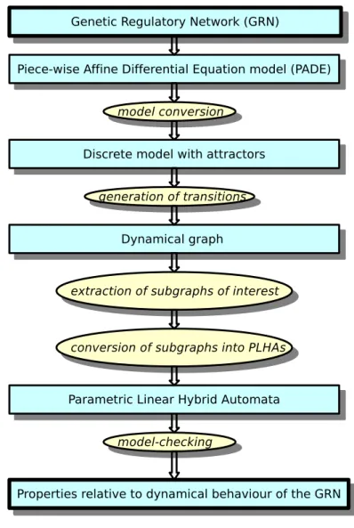
Attempts to model Gene Regulatory Networks (GRNs) have yielded very different approaches. Among others, variants of Thomas’s asynchronous boolean approach have been proposed, to better fit the dy-namics of biological systems: notably, genes were allowed to reach different discrete expression levels, depending on the states of other genes, called the regulators: thus, activations and inhibitions are trig-gered conditionally on the proper expression levels of these regulators. In contrast, some fine-grained propositions have focused on the molecular level as modelling the evolution of biological compound con-centrations through differential equation systems. Both approaches are limited. The first one leads to an oversimplification of the system, whereas the second is incapable to tackle largeGRNs. In this context, hybrid paradigms, that mix discrete and continuous features underlying distinct biological properties, achieve significant advances for investigating biological properties. One of these hybrid formalisms pro-poses to focus, within aGRNabstraction, on the time delay to pass from a gene expression level to the next. Until now, no research work has been carried out, which attempts to benefit from the modelling of aGRNby differential equations, converting it into a multi-valued logical formalism of Thomas, with the aim of performing biological applications. The present research work fills this gap by describing a whole pipelined process which supervises the following stages: (i) model conversion from a Piece-wise Affine Differential Equation (PADE) modelization scheme into a discrete model with attractors (and generation of the corresponune pour la journ´ee portes ouvertes de PolyTech ?ding dynamical graph), (ii) on the basis of probabilistic criteria, extraction of subgraphs of interest from the former dynamical graph, (iii) con-version of the subgraphs into Parametric Linear Hybrid Automata, (iv) analysis of dynamical properties (e.g. cyclic behaviours) using hybrid model-checking techniques. The present work is the outcome of a methodological investigation launched to cope with theGRNresponsible for the reaction of Escherichia
coli bacterium to carbon starvation. As expected, we retrieve a remarkable cycle already exhibited by a
previous analysis of thePADEmodel. Above all, hybrid model-checking enables us to discover additional insightful results, whose interpretations are in accordance with biological evidences.
Due to their equally important complementary contributions, the authors would emphasize that the order chosen for the author list is the alphabetical order.
Introduction
A Gene Regulatory Network (GRN) is a collection of macromolecular compounds such asDNA
and proteins, which functionally interact with each other in a cell. Some proteins, the transcrip-tion factors (TFs), serve only to activate genes and are therefore the main players in regulatory
networks or cascades. By binding to the promoter region in the regulatory region of other genes,
TFs turn the latter on, initiating the production of another protein, and so on. Some TFs are inhibitory. These interactions thereby govern the rates at which genes in the network are tran-scribed into mRNA...
In the simplest cases - that is when interactions do not involve more than two compounds at a time -, aGRNis typically described as a simple directed graph whose vertices are the compo-nents (for illustration, see Figure2(a)). The existence of a labelled directed edge between a pair of genes symbolizes an activation (+) or an inhibition (-) exerted by a gene over another gene through a protein production; besides, the label also mentions the expression level of the regula-tor gene for which the regulation (activation or inhibition) is triggered. Note that a non-inhibiting status is equivalent to an activating status, and symmetrically. Besides, a gene may contribute to activate another gene, together with other co-activators. A gene may also be the co-inhibitor of another gene. More generally, the co-regulation of a given gene is likely to involve activa-tors as well as inhibiactiva-tors. Since regulation is triggered depending on gene expression levels, the regulation of a given gene may involve various sets of co-regulator genes throughout the whole biological system’s life. Hereafter, such set of genes will be called a resource for the regulated gene. In summary, given the current activating or inhibiting statuses of potentially co-regulating genes, a GRN determines the expression level of the gene under regulation, itself a potential regulator for other genes. In this regulatory context, investigating the respective behaviours of genes remains a key question.
Various models of GRNs have been developed to capture the behaviour of the system be-ing modeled, and infer dynamical properties (see de (Jong, 2002) for a review). The followbe-ing modelling techniques used include Boolean networks (Kauffman, 1993), Petri nets (Chaouiya, 2007), Bayesian networks (Hartemink et al., 2001; Yu et al., 2002), graphical Gaussian mod-els (Markowetz et al., 2005), Stochastic (Golightly et al., 2006) and Process Calculi (Kuttler
et al., 2006). The most realistic dynamical models lie on differential equation systems dealing
with protein productions that activate or repress genes. However, such modelling is not im-plementable for realistic biological systems, due to many unknown parameters. Thus, various alternative modelling approaches were proposed. Discretizing protein concentration by thresh-olds quickly appeared as an attractive lead. Henceforth, we will indifferently refer to protein concentration levels or gene expression thresholds. Two categories of approaches implement such a discretized approximation. On the one hand, qualitative methods based on
Piecewise-Affine Differential Equations (PADEs) showed relevant enough to overcome the lack of quanti-tative data on kinetic parameters and molecular concentrations and to fit biologists’expectations (Glass et al., 1973; Snoussi, 1989; de Jong et al., 2004; Batt et al., 2005). On the other hand, an approach first proposed by Thomas combines discretization (both in terms of gene expression levels and time) with the attractor concept (Thomas et al., 1990; Thomas, 1991; Snoussi et al., 1993; Thomas et al., 1995). The definition of this concept will be briefly recalled in the sequel. Time is viewed as proceeding in discrete steps. At each instant t, the current expression levels
of theGRN’s genes determine the genes’ attractors, which are the thresholds towards which the genes’expression levels tend to evolve and which will therefore be assigned to genes at instant
t + 1.
However, some processes, and among them, gene transcription, involve many biochemical reactions or may be delayed until the appropriate molecules are available, which can take time due to possible low concentrations of the latter in the cell. Now, the discrete model with attrac-tors originally proposed implements instantaneous variations of the thresholds. In an ideal model based on discretization, transitions between expression level thresholds would be modelled as sigmoidal functions of the time. Due to unknown tuning parameters, this model is generally not implementable for realistic biological systems. An approximated model has thus been designed to cope with delays; it implements linear variations between genes’thresholds.
In this report, we tackle the problem of describing a realisticGRN through the approach of Thomas, extended with delays. The ultimate aim is identifying essential features of the dynam-ical behaviour of theGRNstudied, using model-checking techniques. As a case study example, we analyse theGRNof the nutritional stress response in Escherichia coli bacterium. Though this
GRNhas been widely studied, the relation between the growth of E. coli and the availability of carbon source is still little understood.
In our approach, the discrete model is built from a formerly publishedPADEmodel (Ropers, 2006), thus benefitting from its parameter tuning. Besides, as the set of global states obtained as well as the transition graph are huge, our work is also novel in that it copes with this difficulty, implementing a complementary probabilistic approach: the latter is used to highlight subgraphs showing characterized states. Then, any such subgraph can be converted into a hybrid model with delays, for the purpose of behavioural property inference. Model-checking tools can be used to analyse these hybrid models.
We first describe the method implementing the conversion of a Piecewise-Affine Differen-tial Equation model into a discrete model with attractors (Section 2). Nevertheless, the dis-crete model of a large GRN is not easily tractable for property inference implemented through model-checking techniques. Therefore, in Section 3, a method dedicated to the extraction of
subgraphs of interest in the dynamical graph is proposed. This process is performed on the basis of a probabilistic rationale and identifies subgraphs characterized with remarkable states. Then, Section4 focuses on the integration of delays into the discrete model, leading to an hybrid
sys-tem. Throughout our exposition, the simplicist regulation system for bacterium Pseudomonas
aeruginosa’s mucus production will be used for illustration. The outcome of our
methodolog-ical approach is the processing scheme depicted in Figure1. In Section 5, we apply the whole
Therein, we present and discuss insightful results obtained for this realistic case, originally the instigator case for the pipelined process design.
1
Conversion of a
PADEmodel into a model with attractors
1.1 PADE model
We first recall how the concentration evolution of a protein regulated by aGRNcan be modelled
through a Piece-wise Affine Differential Equation (Snoussi, 1989; de Jong et al., 2001). PADE
modelling relies on discretization: for each proteini, its concentration is known to evolve within
a domain discretized into an ordered set of thresholdsθ1, θ2...
Definition 1 (Evolution of protein concentration)
Typically, the evolution of concentrationxiwith time is expressed as: ˙xi = fi(x) − γixi, 1 ≤
i ≤ n, xi ≥ 0,
wherex = (x1, . . . , xn) is a vector of n protein concentrations. The equation above relates the
concentration modification rate ˙xito a synthesis rate,fi(x), and a degradation rate, γixi.
Functions fi express the dependence of xi upon the concentrations of other constituents
present in the cell. Such functions are derived from basic principles of chemical kinetics, in-cluding for example Michaelis-Menten enzymatic kinetics.
Notation 1 (Resource set)
In the following,R(i) will denote the set of all resources likely to regulate gene i. A resource for
genei is itself a set of genes (possibly inclusing gene i) involved in the co-regulation of gene i.
Definition 2 (Description of regulation)
fi(x) expresses the synthesis rate of component i as a function of the concentrations of regulator
genes inithgene’s resources:
fi(x) = ki+Pr∈R(i)kirbir(x), ki ∈ R+∗, kir∈ R+, bir∈ {0, 1},
wherekiandkirare kinetic parameters.
Switching the boolean parameter bir(x) to 1 means that the corresponding resource r is
active, that is each generjbelonging to the resource setr is either an activator or a non-inhibitor
for genei, depending on its concentration xrj. Switchingbir(x) from 0 to 1 and symmetrically
relies on the satisfaction of constraints by the concentrations relative to the genes belonging to resource setr. In a discrete framework, such constraints are expressed through concentration
thresholds.
Before we may further explain how entities bir describe regulator contributions, we need
detail the concept of discretization. Such concentration thresholds aforecited are defined as follows:
Definition 3 (Discrete concentration thresholds)
Figure 1: The pipelined process designed for the analysis of largeGRNs.
For genej characterized by τj thresholds, the following ordered relation is verified:0 < θj1 < θj2 < · · · < θjτj.
Any such set of thresholds defines a set of domains, further called local states, traversed by the system under study, when considering only genej. More generally, this system evolves through
global states, which refer to all possible combinations of local states associated with the genes in the system. Such previous concepts establish the notion of discrete dynamics of the system.
Then, thebir(x) terms in Definition 2.2 will be tailored as functions of entities defined as
Definition 4 (Step function)
Givenrj, a regulator gene belonging to resourcer, and one of its τj thresholdsθrjα,
s+(xrj, θrjα) = ( 1, if xrj ≥ θrjα 0, if xrj < θrjα s−(xrj, θrjα) = 1 − s +(x rj, θrjα).
Finally, any co-regulation involving the genes of a resource setr may be modelled adapting biras a combination of various step functions s+and s−. The following grammar enumerates
all possible combinations:
bir ::= comb
comb ::= s+| s−| 1 − comb | comb comb.
Through the bir coefficients, the activation or inhibition sigmoidal functions are
approxi-mated into piece-wise linear functions.
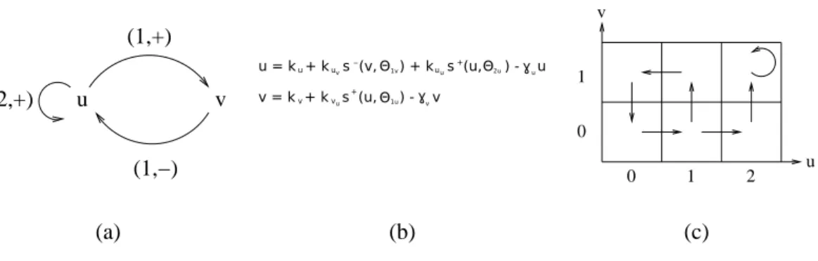
For a didactic exposition, we will illustrate the various concepts used throughout this article with the simpleGRNinvolved in the mucus production of bacterium P. aeruginosa. Figure2(b) presents thePADEmodel corresponding to theGRNdescribed in Figure2(a).
u v (2,+) (1,+) (1,−) 0 1 2 0 1 u v (a) (b) (c)
Figure 2: Regulation of the mucus production for P. aeruginosa bacterium (a) labelled GRN;
(b) Piece-wise Affine Differential Equation model (PADE); (c) asynchronous discrete model. (a) The directed edgeu → v labelled with (1, +) means that u activates v as soon as u’s expression
level reaches the threshold value of1. The directed edge v → u labelled with (1, −) indicates
that the inhibition ofu by v is triggered as soon as v’s expression level is 1. Note the positive
feedback loop foru.
1.2 Discrete model with attractors
In the abstract semi-qualitative model of Thomas, each gene expression variation domain is discretized using appropriate thresholds. The knowledge of all such gene thresholds is the pre-requisite for building the graph whose dynamical behaviours will be studied. Global states are directly inferred identifying all valid threshold combinations. In particular, biological knowl-edge allows discarding global states which do not exist: for example, antagonist components
can not show simultaneously high (resp. low) expression levels or concentrations. Once the valid global states of the dynamical graph are identified, its transitions have to be inferred. In the model inspired from that proposed by Thomas, the dynamical aspect is modelled through the attractor concept.
Definition 5 (Attractor)
In a given global states, a gene u is associated to a specific attractor value, representing the
expression level towards which this gene will tend to evolve, starting from su, its expression
level in global states. The evolution of gene u depends upon one or more other genes, together
defining the resource setr(u, s) for u in global state s. Therefore, the attractor value of gene u, Ku,r(u,s), is related tou’s resource.
Table1recapitulates the three possible evolution tendencies for geneu.
su < Ku,r(u,s) The expression level ofu tends to increase.
su = Ku,r(u,s) The expression level ofu is steady.
su > Ku,r(u,s) The expression level ofu tends to diminish.
Table 1: Determination of the tendency for geneu, depending on its expression level su and its
attractor valueKu,r(u,s), in global states. r(u, s) denotes the resource set of gene u, in global
states.
Knowing these tendencies for all genes and for all global states is the key to infer the tran-sitions of the dynamical graph. Central to any modelling paradigm using discretization is the concept of qualitative focal point.
Definition 6 (Qualitative focal point)
In global state s, with each gene u of the system evolving towards its attractor value Ku,r(u,s),
the qualitative focal point is defined as the vector (Ku1,r(u1,s), · · · , Kun,r(un,s)). Any focal point
is uniquely associated with an abstract region in the discretized hypercube of dimensionn, where
each dimension describes local state traversing for one of then genes of the system.
A most difficult task remains in tuning attractor values: usually, instanciating attractor values for a given global state is an under-constrained problem. Biological knowledge together with Snoussi constraints prohibit some instanciations (Snoussi constraints specify that the addition of supplementary activating (resp. inhibiting) resources for a given gene obligatorily leads to the increase (resp. decrease) of its attractor value). Table 2shows a possible instanciation for theGRN illustrated in Figure2(a). In the asynchronous model, best consonant with biological reality, a change of state is only allowed for at most one gene along each transition. As a result, if a global states is its own successor, it is a steady global state whereas it possesses p successors
if tendency to evolve is detected forp genes. Figure2(c) provides the asynchronous description derived from the tendencies of Table2.
u v attractor foru attractor forv tendency forv tendency foru 0 0 Ku,{v} = 2 Kv,{}= 0 ր → 0 1 Ku,{}= 0 Kv,{}= 0 → ց 1 0 Ku,{v} = 2 Kv,{u}= 1 ր ր 1 1 Ku,{}= 0 Kv,{u}= 1 ց → 2 0 Ku,{u,v}= 2 Kv,{u}= 1 → ր 2 1 Ku,{u}= 2 Kv,{u}= 1 → → an instanciated model:
Ku,{}= 0, Ku,{v} = 2, Ku,{u,v}= 2, Kv,{}= 0, Kv,{u}= 1
Table 2: A possible instanciation of attractors, for theGRNof Figure2(a). We explain the third line relative to global state(su = 1, sv = 0): since v is not inhibiting u (sv < 1), v activates
u as its only resource; u being in state 1, a consistent instanciation for Ku,{v}is thus the value
of2; the condition is required for u’s activation of v (su≥ 1) and a coherent value for Kv,{u}is
therefore1. In conclusion, both gene expressions tend to increase.
1.3 Model conversion
The key to the conversion of a PADE model into a discrete model with attractors relies on the quasi-straightforward determination of such attractors from the differential equations, as well as a facility to instanciate them through the set of constraints associated with these equations. Indeed, the qualitative focal point of Thomas’s formalism coincides with the abstract region (in the hypercube of dimensionn) containing the steady state for thePADEsystem.
Proposition 1 (Conversion rule)
Referring to thePADErelated to genei (definitions 2.1 and 2.2 combined), ˙xi = ki+Pr∈R(i)kirbir(x)−
γixi, 1 ≤ i ≤ n, xi ≥ 0, bir ∈ {0, 1}, we obtain the attractor value of gene i in global
states when ˙xi is equal to0 (steady state) and bi,r(i,s)(x) is switched to 1 due to the activating
regulation of resourcer(i, s) :
Ki,r(i,s)= Di(
ki+Pr∈R(i)∩r(i,s)kir
γi
),
where the discretization function Diconverts the ratio into one of theτiθiαthresholds associated
with genei.
Example 1
When applied to the case of P. aeruginosa’s mucus production regulation (see Table 3), the conversion process exploits constraints relative to thresholds ((3) to (4)) as well as kinetic parameters ((5) to (8)).
(1) ˙u = ku+ kuv s−(v, θ1v) + kuus+(u, θ2u) − γuu (2) ˙v = kv+ kvu s +(u, θ1 u) − γvv (3) 0 ≤ θ1u< θ2u ≤ maxu (4) 0 ≤ θ1v ≤ maxv (5) 0 ≤ ku γu ≤ θ1u (6) θ2u≤ ku+kγuuv + ku+kγuuu +ku+kuvγu+kuu ≤ maxu (7) 0 ≤ kv γv ≤ θ1v (8) θ1v ≤ kv+kγvvu ≤ maxv (9) Ku,{}= Du(kγuu) (10) Ku,{u}= Du(ku+kγuuu) (11) Ku,{v}= Du(ku+kγuuv) (12) Ku,{u,v}= Du(ku+kuuγu+kuv) (13) Kv,{}= Dv(kγvv) (14) Kv,{u}= Dv(kv+kγvvu)
Table 3: Identification of resources and tuning of attractors from thePADE of Figure2(b). At-tractors are easily identified from equations (1) and (2): in addition toKu,{v},Ku,{u}andKv,{u},
attractors corresponding to the absence of resource are Ku,{} and Kv,{}. Moreover, attractor
Ku,{u,v}has to be created. It follows from equations (3) to (8) and from Snoussi constraints (
Ku,{} ≤ Ku,{v} ≤ Ku,{u, v},Ku,{} ≤ Ku,{u} ≤ Ku,{u,v}and Kv,{} ≤ Kv,{u}) that one of the
possible instanciations is the one deduced in Table 2. Du and Dv are discretization functions
2
Extraction of subgraphs of interest
We implemented a coloration method designed to highlight the most interesting states of the dynamical graph. This method relies on a probabilistic rationale.
Turning the dynamical state graph initialy obtained into a Markov chain is straightforward. For each transition originating from a given global statei (1 ≤ i ≤ N ), a probability is computed
as the inverse of the outter degree of statei. Formerly, the transition matrix M of the Markov
chain associated to the dynamical graph denotedG = (V, E) satisfies ∀i, j ∈ V, Mj,i =
[[i → j ∈ E]] #{k, i → k ∈ E},
where[[B]] = 1 if property B is true and 0 otherwise (Iverson’s notation) and #{k, i → k ∈ E}
is the outter degree of statei.
Next, we define the steady-state probability P⋆ as
P⋆ = lim ℓ→∞ 1 N ℓ X i=0 MiF,
whereF is the vector of initial probabilities (in the sequel, this vector is set as Fi = 1/|V |,
1 ≤ i ≤ N .). Here, the sum ensures the convergence to a unique probability distribution, even
in the case of a non irreducible or periodic Markov chain.
We use the steady-state probability P⋆ to highlight vertices in G (i.e. the global states of
the dynamical graph). Relying on steady-state probabilities is justified by their being closely related to the number of times the different states are traversed in infinite random trajectories. Consequently, the higher is such a probability, the more important would be the associated state, with regard to the system’s behaviour.
As infinite trajectories do not make sense in a biological context, it is more relevant instead to focus on finite trajectories. We define the vector Pℓofℓ-finite state probabilities to be
Pℓ= 1 ℓ ℓ X i=0 MiF,
whereF is the vector of initial probabilities.
Theℓ-finite state probability Pℓ[i] is proportional to the mean number of times a given state
i is traversed.
Notice that we thus provide a way to colorize the dynamical state graph by assigning to each statei a colour value proportional to Pℓ[i]. For long trajectories, when ℓ is approximately
the number of states in the graph, the states supposedly most crucial to the biological system’s behaviour are emphasized. In an automated approach, we use vector Pℓ to prune the dynamical graph by extracting the induced subgraphs composed of statesi such that Pℓ[i] > 2/N . Each
E. coli response to carbon deprivation, this cut off threshold of2/N ensures that the subgraphs
obtained are tractable for any further analysis.
3
Extending the discrete model paradigm with delays: the hybrid
model
3.1 Clocks and delays
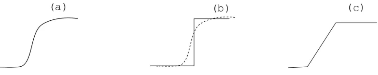
The evolution of the expression of a given gene is a continuous non-linear process (see Figure3). This fact is not taken into account in the discrete modelling formalism of Thomas, where gene expression evolves from one level to another level in a discrete fashion (see Figure3(b)). In the field of biological modelling, paradigms have been proposed to simulate continuous temporal evolution (Bernot et al., 2004; Adela¨ıde et al., 2004; Siebert et al., 2006). The refinement of discrete modelling by a more enhanced formalism of hybrid modelling has been proposed (Ahmad et al., 2007), in which the sigmoid-like evolution is no more approximated by a discrete step but by a piece-wise linear curve instead (Figure3(c)). Since we now consider that the delay needed for a gene to evolve from expression levela to a + 1 or a − 1 is not null, we have to deal
with additional concepts, namely time intervals and clocks.
Figure 3: A sigmoid relation (a) and its discrete (b) and piece-wise linear (c) approximations.
The widely-spread timed automaton formalism provides a formal framework to describe hybrid systems (Alur et al., 1994). In this framework, any global state of the system modeled is described by a discrete spacial location (in our case, the vector of current gene expression values) and a vector of continuous variables, called clocks. Any geneu is associated to a clock (denoted hu). Evolving synchronously with time, clock intervals therefore superimpose a representation
of continuous system’s dynamics on the already defined discrete dynamics. The clocks act as transition guards and are reset to0 when the system passes from one discrete location to another
one. The more general class of Linear Hybrid Automata (LHA) is the appropriate framework allowing the definition of time interval associated to a clock (Henzinger et al., 1995). For any clock, its current value measures the time elapsed since the most recent change occurred for the system, in the discrete space of gene expressions. Thus, if the system consists ofn genes, an
LHAformalism superimposes a temporal hypercube of dimensionn to the discrete global state
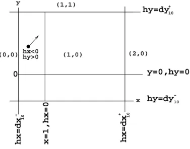
space. For illustration, in dimension2, a global state is now associated to a rectangular temporal
level is a real parameter depending onu’s current discrete state (du+ > 0); symmetricaly, the
delay to decrease down to next discrete level is| du−| (du−< 0).
(2,0) (0,0) (1,1) hx=dx hx=dx y=0,hy=0 hy=dy hy=dy (1,0) 10 10 10 10 + + − − y x x=1,hx=0 0 hx<0 hy>0
Figure 4: Hybrid model - temporal regions and delays -. Here, global state(x, y) = (1, 0) is
associated to delaysdx+10,dx−10,dy+10anddy−10.
To model time elapsing, we use a subclass of theLHA formalism, which associates to each geneu a clock rate, ˙hu, in the restricted set{−1, 0, 1}. Rates −1, 0 and 1 respectively signify
that gene expression level is decreasing, staying at the same level or increasing. Any clock rate
˙
hu related to geneu indicates the evolution tendency for this gene, with respect to the current
global state. Prior to any analysis of the dynamical behaviour of the modeled system, each such clock rate must be tuned. In contrast with the asynchronous discrete model of Thomas, tuning the clock rates now requires looking several steps ahead in the dynamical graph, in order to capture the whole actual tendency. For instance, in Figure2(c), if one confines to a depth of2
to examine next transitions, when starting from state(0, 1), as u decreases and v increases, ˙hu
and ˙hvare respectively set to1 and −1 (see (Ahmad et al., 2007) for details).
Delays being considered as parameters, such a model will be called a Parametric Linear Hybrid Automaton (PLHA) in the sequel. Now all concepts have been unformally introduced and illustrated, next subsection will rigorously definePLHAs together with their semantics.
3.2 Parametric Linear Hybrid Automata
We remind the reader that derivative ˙x denotes the evolution rate for protein concentration x
while ˙hx is the evolution rate of the clockhxassociated with variablex.
Notation 2
is a formula of the formx ⊲⊳ c, for x ∈ X, c ∈ Q∪P and ⊲⊳ ∈ {<, ≤, ≥, >}. We denote C(X, P )
the set of constraints over a set of variablesX and parameters P , which consists of conjunctions
of atomic constraints. Given a constraintg, we let V(g) be the set of variables that appear in g.
We letC=(X, P ) (resp. C≤(X, P ), C≥(X, P )) be the set of constraints using only = (resp. ≤,
≥).
Definition 7 (PLHA)
APLHAis a tuple(L, ℓ0, X, P, E, Inv, Dif ) defined as follows:
• L is a finite set of locations
• ℓ0 ∈ L is the initial location
• P is a finite set of delay parameters
• X is a finite set of clocks
• E ⊆ L × C=(X, P ) × 2X× L is a finite set of edges, e = (ℓ, g, R, ℓ′) ∈ E represents an
edge from locationℓ to location ℓ′, associated with the guardg and the reset set R ⊆ X
(we require thatV(g) ⊆ R)
• Inv: L → C≤(X, P ) ∪ C≥(X, P ) assigns an invariant to any location
• Dif: L × X → {−1, 0, 1} maps each pair (ℓ, x) to an evolution rate.
The semantics of aPLHA is a timed transition system. It is defined according to the time domain T. We let T∗ = T \ {0}.
Definition 8 (Semantics of aPLHA)
Letγ be a valuation for the parameters P . The (T, γ)–semantics of a parametric LHA H =
(L, ℓ0, X, P, E, Inv, Dif) is defined as a timed transition system SH = (S, s0, T, →) where: (1)
S = {(ℓ, ν) | ℓ ∈ L and ν |= Inv(ℓ)}; (2) s0 = (ℓ0, ν0) with ν0(x) = 0 for every x ∈ X; (3)
the relation→ ⊆ S × T × S is defined for t ∈ T as:
• discrete transitions:(ℓ, ν)→ (ℓ0 ′, ν′) iff ∃(ℓ, g, R, ℓ′) ∈ E such that γ(ν) = true, ν′(x) = 0 if x ∈ R and ν′(x) = ν(x) if x /∈ R.
• continuous transitions: Fort ∈ T∗,(ℓ, ν)→ (ℓt ′, ν′) iff ℓ′ = ℓ, ν′(x) = ν(x) + Dif(ℓ, x) ×
t, and for every t′ ∈ [0, t], (ν(x) + Dif(ℓ, x) × t′) |= Inv(ℓ).
The semantics of a PLHA implements two types of transitions: discrete and continuous. Invariants and guards are constraints set on subsets of clocks. Invariants specify the conditions under which the system is allowed to stay in the current state, while time elapses. A discrete
transition is an instantaneous transition that occurs between two discrete locations. It is fired
when the associated guard is satisfied. Continuous transitions account for elapsing of time in a discrete location until the associated invariant condition is no more satisfied. A continuous transition allows the updating of the clocks in any time interval[0, t], according to the evolution
rates specified for the clocks and provided that the invariant conditions are still verified. We refer the reader to appendix1 for the formal definition of the semantics ofPLHAs.
Example 2 (PLHA)
The Parametric Linear Hybrid Automaton of the example of P. aeruginosa (see Figure 2) is shown in Figure5. Here, the delays are represented by the notationdα
i,ℓ, whereα denotes the
delay sign (+ for activation and − for inhibition) of a gene i in a location ℓ. This automaton
has six locations. The locations are labelled with the invariant conditions while the discrete transitions are labelled with guards and clock resets.
(0,1) d -v,(0,1) hv < V d+u,(0,1) hu < = 1 , hu hv = -1
.
.
d+ v,(0,0) hv < d+u,(0,0) hu < V (0,0) = 1 , hu hv = 1.
.
d+ v,(1,0) hv < d+u,(1,0) hu < = 1 , hu hv = 1.
.
V (1,0) d+ v,(2,0) hv < = 0 , hu hv = 1.
.
(2,0) d-u,(1,1) hu < hv < d-v,(1,1) = -1 , hu hv = -1.
.
V (1,1) d+u,(1,0) hu hu 0 == d + v,(2,0) hv == hv 0 d+u,(0,0) hu d -v,(0,1) h ==v d-u,(1,1) hu== hu 0 h v 0 hu 0 == d + v,(1,0) hv == hv 0 = 0 , hu hv = 0.
.
(2,1)Figure 5: Hybrid model for P. aeruginosa mucus production.
3.3 Automatic symbolic analysis of aPLHAthrough HyTech model-checker
HyTech is the model-checker chosen in our study (Henzinger et al., 1997). It is adapted to
hybrid systems: it has the ability to manage parameters through synthesizing constraints relative to these parameters, thus satisfying necessary conditions for the existence of the behaviours analysed.
Definition 9 (Trajectories and cycles)
A trajectory is a sequence of states related by discrete and continuous transitions. A cycle is a trajectory that starts in a given location and returns to this same location further on.
In the hybrid model of aGRN, we respectively denoteϕ(t) for t ∈ R≥0and S the sequence
of points of a trajectory and the set of all points in its state space.
Definition 10 (Invariance kernel)
A trajectoryϕ(t) is viable in S if ϕ(t) ∈ S for all t ≥ 0. A subset K of S is said to be invariant
if for any pointp ∈ K, a trajectory starting in p is viable in K. An invariance kernel K is the
largest invariant subset of S.
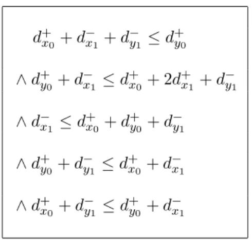
For illustration, the set of constraints displayed in Table4characterizes the invariance kernel of the example relative to P. aeruginosa (see Figure2). For the sake of simplicity, we only deal
with few delay parameters, assuming that alldαij are equal, whatever the actual value ofj, and
similarly for alldα
ij, whatever the actual value ofi.
d+x0+ d−x1 + d−y1 ≤ d+y0 ∧ d+y0 + d−x1 ≤ dx+0 + 2d+x1 + d−y1 ∧ d−x1 ≤ d + x0+ d + y0 + d − y1 ∧ d+y0 + d − y1 ≤ d + x0+ d − x1 ∧ d+ x0 + d − y1 ≤ d + y0 + d − x1
Table 4: Delay constraints characterizing the invariance kernel of P. aeruginosa.
4
The pipelined process applied to the analysis of the reaction of E.
coli to carbon availability
We recall the reader that the pipeline process implemented schedules the following tasks: (i) con-version from a PADE model to a model with attractors, (ii) identification of the corresponding transition graph, (iii) identification of induced subgraphs of interest in the former graph, imple-mented through a probabilistic approach, (iv) modelization of subgraphs in the framework of
PLHAformalism, (v) analysis of characterized dynamical behaviours through HyT ech
model-checker. Note that third step actually provides a visualization tool able to point out subgraphs containing global states of interest.
It must be emphasized that our contribution is the first example of an application of timed-model checking techniques on the case of E. coli regulation related to carbon availability. Indeed, the former works relative to thisGRNdid not take into account the concept of delays (Batt et al.
2005).
The implementation of the protocol previously described provides multiple significant re-sults in the case of E. coli response to carbon availability.
4.1 ThePADE model of the carbon starvation response in Escherichia Coli
The growth of bacterial populations is related to the quantity of nutrients present in their environ-ment. Nutrient availability entails an exponential increase of the prokaryotic biomass whereas nutritional stress induces growth deceleration or even growth stop. Thus, bacterial populations are subject to transitions between two states denoted as exponential and stationary phases
re-spectively. The switch between these two phases is crucial to bacterial survival and is controlled by aGRNthat integrates various environmental signals.
TheGRNcontrolling the response to carbon deprivation has been widely studied E. Coli, in the past decades. In contrast to most studies focusing on only one or a few components of this network, Ropers and co-authors’recent contribution implemented the modelling of concentration evolution for six key global regulators of this network (Ropers et al., 2006). This model relates the behaviours of five genes (crp, cya, f is, gyrAB, topA) and two supplementary ”signals”
such as the carbon starvation information and the quantity of stableRNAs. The reader interested
in details about the biological hypotheses used for describing the genetic interactions is referred to (Ropers et al., 2006).
The PADEmodel of Ropers and co-workers was shown to fit to typical features describing the transition between bacterial growth phases. We therefore admit that this model was validated and we used a slightly simplified version as a starting point to establish a more refined modelling approach based on attractors and delays. The simplified version of thePADEmodel adapted from Ropers and co-workers’model is shown in Table5. Herein, we present the simplified equations together with their associated constraints. As the variablexrrn corresponding to stable RNAs
had no influence on others variables, it was discarded from our ownPADEmodel. In addition, we dismissed three thresholds, θ3crp, θ3cya and θ5f is, which appeared to be useless. Thus,
contraints applying toθ3crp now apply toθ2crp; similarly, θ2cya is constrained as was θ3cya;
finally, parameter inequalities relative to the formerθ5f isnow apply toθ4f is.
4.1.1 Conversion of the PADE model relative to E. coli response to nutrient availability into a discrete model with attractors
Benefitting from a previousPADE modelling of E. coli response to carbon availability, we are thus able to skip the tedious task of identifying attractors ab initio. Moreover, the instanciation is facilitated by the set of constraints associated with the PADE model. Indeed, provided that
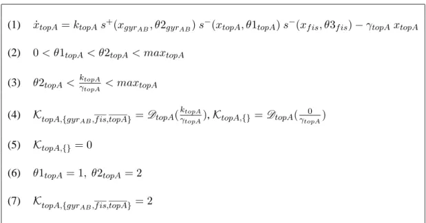
we understand how to relate the kinetic parameters and the degradation rate of thePADEsystem with attractor values, the instanciation process will be significantly simplified. Table6focuses on an excerpt of Ropers and co-authors’model (in its simplified version).
The equation in line (1) models the variation ofxtopA, that is the concentration of
topoi-somerase. For the sake of simplicity, Ropers and co-authors considered that a single promoter is involved in the expression oftopA gene, whereas there are indeed five promoters involved
in its expression. The expression of this gene is also controlled by antagonistic agents: topA
is activated by a low level off is; in contrast, it is activated by a high level of gyrAB. Two
different thresholds have been considered in the simplified version, θ1topA and θ2topA.
Stim-ulation of topA promoter by its resource {gyrAB, f is, topA}, where the first gene is
activat-ing and the two others are not inhibitactivat-ing, entails maximal production oftopA. It follows that θ2topA<
ktopA
˙us= 0
˙xcrp= k1crp+ k2crps−(xf is, θ2f is) s+(xcya, θ1cya) s+(us, θs) + k3crps−(xf is, θ1f is) − γcrpxcrp 0 < θ1crp< θ2crp< maxcrp θ1crp< k1crp γcrp < θ2crp θ1crp< k1crp+k2crp γcrp < θ2crp θ2crp< k1crp+k3crp γcrp < maxcrp θ2crp< k1crp+k2crp+k3crp γcrp < maxcrp
˙xcya= k1cya+ k2cya(1 − s+(xcrp, θ2crp) s+(xcya, θ2cya) s+(us, θs)) − γcyaxcya 0 < θ1cya< θ2cya< maxcya
θ1cya<k1cya
γcya < θ2cya
θ2cya<k1cya+k2cya
γcya < maxcya
˙xf is= k1f is(1 − s+(xcrp, θ1crp) s+(xcya, θ1cya) s+(us, θs)) s−(xf is, θ4f is) +k2f iss+(xgyr
AB, θ1gyrAB) s
−(xtopA, θ2topA) s−(xf is, θ4f is) (1 − s+(xcrp, θ1crp) s+(xcya, θ1cya) s+(us, θs)) − γf isxf is 0 < θ1f is< θ2f is< θ3f is< θ4f is< maxf is
θ1f is<k1f is
γf is < θ2f is
θ4f is<k1f is+k2f is
γf is < maxf is
˙xgyrAB = kgyrAB(1 − s+(xgyrAB, θ2gyrAB) s−(xtopA, θ1topA)) s−(xf is, θ3f is) − γgyrABxgyrAB
0 < θ1gyrAB< θ2gyrAB < maxgyrAB
θ2gyrAB<
kgyrAB
γgyrAB < maxgyrAB
˙xtopA= ktopAs+(xgyrAB, θ2gyrAB) s
−(xtopA, θ1topA) s−(xf is, θ3f is) − γtopAxtopA 0 < θ1topA< θ2topA< maxtopA
θ2topA<ktopA
γtopA < maxtopA
Table 5: Equations and associated constraints depicting the simplified model adapted from Rop-ers and co-authors, to simulate the response to carbon deprivation in Escherichia coli. The five variables correspond to protein concentrations: xcrp(CRP),xcya(Cya),xf is(Fis),xgyrAB
(GyrAB),xtopA(TopA).
Applying this process to each equation in the PADEsystem of Table 5, we finally obtain a discrete model with instanciated attractor values. As explained in subsection 1.2, the construc-tion of the dynamical graph is now straightforward. However, as foreseeable for such a complex
GRNas E.coli reponse to nutrient availability, before behavioural property inference may be per-formed through model-checking techniques, a simplification stage is required. For example, the dynamical graph corresponding to E. coli response to nutrient availability contains such a high numberN of vertices (i.e. states) as 810.
(1) ˙xtopA= ktopAs+(xgyrAB, θ2gyrAB) s
−(x
topA, θ1topA) s−(xf is, θ3f is) − γtopAxtopA
(2) 0 < θ1topA< θ2topA< maxtopA
(3) θ2topA< ktopA
γtopA < maxtopA
(4) KtopA,{gyr
AB,f is,topA} = DtopA(
ktopA
γtopA), KtopA,{}= DtopA(
0 γtopA) (5) KtopA,{}= 0 (6) θ1topA= 1, θ2topA= 2 (7) KtopA,{gyr AB,f is,topA} = 2
Table 6: Identification of resources and tuning of attractors for the response to carbone starva-tion in E. coli. The differential equastarva-tion of Ropers’model (1) allows the identificastarva-tion of the two attractors concerned (4). DtopAis a function used to obtain an integer attractor value
(discretiza-tion). AttractorKtopA,{}(5), corresponding to the case when no resource is available, is trivially instanciated with the value of0; together with conversion rule (3), Ropers’s constraints (2)
in-duce the instanciation of concentration thresholds (6); finally, a value of2 is an instanciation of KtopA,{gyr
AB,f is,topA}attractor’s value consistent with (3), (4) and (6) constraints.
4.2 The initial dynamical graph
The entire transition graph contains 810 global states and 3827 transitions. However, the
dy-namics of the exponential phase and that of the stationary phase are to be studied separately. Indeed, our purpose here is not to focus on transitions switching from one phase to the other one. The graph describing the dynamics of the stationary phase consists of405 global states
and1523 transitions. The graph corresponding to the exponential phase contains 405 states and 1494 transitions. After conversion from thePADEmodel into a discrete model with attractors, we dismissed some states known to be never encountered (crp = 0). In this report, we chose
to concentrate on the exponential phase. The reduced graph describing the dynamics of the exponential phase consists of108 global states.
Incidentally, we checked that some specific properties reported in the literature hold for the model inferred. For example, thecrp/f is antagonism (crp = 2 and f is = 0) is verified as
ex-pected. Besides, it has been checked thatDNAsupercoiling is absent from every cycle belonging
to the graph characterizing the exponential phase: f is = 0 =⇒ topA > gyrAB. Indeed, two
modulates the topology of DNAin a growth-phase dependent manner, to counteract excessive levels of superhelicity (Travers et al., 2001). First, the binding of FIS toDNAconstrains nega-tive superhelicity to low levels; second, a reduction in the expression and effecnega-tiveness ofDNA
gyrase achieves the same result. Conversely, highf is expression levels do themselves require a
high negative superhelical density.
4.3 Extraction of a characterized cycle
When applying the ”coloration” process to the graph related to exponential phase, we identify the subgraph depicted in Figure 6. This subgraph is outstandingly dense in states of interest (i.e. potentially frequently encountered states in long trajectories) and therefore contains several qualitative cycles, among which we recognize a cycle well-known in E. coli response to carbon availability:
012100→ 012110 → 012120 → 012220 → 012320 → 012420 → 012410 → 012400→ 012300 → 012200 → 012100
(the six values respectively correspond tocrp, cya, f is, gyrAB,topA and rrn). Interestingly,
it happens that this cycle corresponds to the one identified by Ropers and co-workers (Ropers et
al., 2006), displayed in Figure7, except that only4 levels are considered for f is.
Moreover,HyT ech model-checking techniques enable us to capture this cycle through the
analysis of invariance kernel in the hybrid model built for the subgraph of Figure6. As stated in the study based onPADEmodelling (Ropers et al., 2006), we show that the system behaviour is likely to end running into the qualitative cycle aforementioned. At this stage, it is remarkable that a graph pruning probabilistic process combined with hybrid modelling on the one hand and
PADEmodelling on the other hand meet to reveal the very same qualitative cycle.
Before commentating on the results obtained throughHyT ech analysis, we have to define
the so-called full period (denotedπ(u)) as the sum of all delays for a gene u to pass sequentially
and successively, once through each of all its expression levels.
It should be noticed that the real time for a gene to run along this route (if it actually takes place) may be greater than the full period since it may include lazy stages, i.e. some time intervals where there is neither increase nor decrease.
4.3.1 Identification of temporal constraints
Restraining tof is and gyrAB, the cycle aforementioned is merely expressed as
+ 1 + 0 → + 1 + 1 → + 1−2 → + 2−2 → + 3−2 →−4−2 →−4−1 →−4 = 0 →−3 + 0 →−2 + 0 → + 1 + 0
where symbols+, − and = indicate the evolution tendency for each gene.
The analysis with HyT ech provides two kinds of results relative to this peculiar cycle.
(1,2,1,0,0) (1,2,1,1,0) (1,2,1,2,0) (1,2,2,1,0) (1,2,2,2,0) (1,2,1,2,1) (1,2,3,2,0) (1,2,3,1,0) (1,2,4,2,0) (1,2,4,1,0) (1,2,3,0,0) (1,2,4,0,0) (1,2,2,0,0)
Figure 6: A subgraph showing cycles in the exponential phase, for E. coli bacterium. The global states are represented in the same manner as in Figure5. The five values respectively correspond tocrp, cya, f is, gyrAB, andtopA. The states of Ropers and co-workers’cycle are highlighted
Figure 7: Qualitative cycle of E. Coli associated with the series of phases denoted Q107s , Q109 s , Q 69 s , Q 71 s , Q 49 s , Q 51 s , Q 39 s , Q 41 s , Q 49 s , Q 43 s , Q 53 s , Q 95 s , Q 105 s © (Ropers, 2006).
registered (1) to (3), in Table7). On the other hand, we exhibit a relation between the lengthL
of this cycle and the delays associated with genes (equalities 4 (a) and 4 (b), in Table7).
4.3.2 Interpretation and relevance with regard to biological evidences
• First, it follows directly from (3) thatπ(gyrAB) ≤ π(f is).
This inequality is explained by the fact that there exists a phase in the cycle wheregyrAB
is lazy (i.e. it stays at the same expression level). This may be observed in the phase
−
4=0 of the cycle, corresponding to the state Q41
s in figure7. Thus, the qualitative cycle in
which E. coli bacterium is involved during the exponential phase following a carbon sup-ply is possible whengyrAB qualitative period is smaller than that off is: therefore, the
path of transitions through minimum to maximum qualitative state and back is traversed faster forgyrAB than forf is. This remark implies that a slight increase of gyrAB’s
pe-riod might not allow the bacterium to stay in the exponential phase. gyrAB is closely
related to DNAsupercoiling. Therefore, slowing down the gyrAB cycle running would
d+f is 1 + d + f is2 + d + f is3 + |d − f is3| + |d − f is2| ≤ d +
gyrAB0 + d+gyrAB1 + |d−gyrAB2|
d+gyrAB0 + d+gyrAB0 ≤ d+f is1 + |d
− f is2| + |d − f is3| d+gyr AB0 + d +
gyrAB1 + |d−gyrAB2| + |d−gyrAB1| ≤ d+f is1 + d
+ f is2 + d + f is3 + |d − f is4| + |d − f is3| + |d − f is2| L = d+f is1 + d+f is2 + d+f is3 + |d−f is4| + |d−f is3| + |d−f is2| L = d+ gyrAB0 + d+f is1 + d + f is2 + d + f is3 + |d − f is4|.
Table 7: Identification of temporal constraints associated with the existence of the cycle high-lighted in Figure6.
impact of theDNA-superhelicity on the bacterial gene activity (see (Hatfield et al., 2002))
for a review). Basal expressions of genes are low when chromosomal superhelical den-sity is low, and conversely. Because of the necesden-sity to react to environmental variation for survival, low bacterial activity acts as a trigger for switching to the stationary phase. This remark confirms the temporal constraint mentioned above as a biological insight. D. Ropers and co-workers depicted this qualitative cycle as an unexpected result. However, our investigation of temporal properties associated with this cycle points out insights that are relevant with biological evidences aboutDNAsupercoiling.
• Second, we deduce from (4) (a) thatL = π(f is) (and hence L ≥ π(gyrAB).)
Thus, we are able to prove that the cycle length is exactly the full period of f is. This
result is consistent with the fact that there is no lazy phase forf is. Moreover, this
obser-vation implies thatf is plays the major role in the qualitative cycle in which the bacterium
is kept during the exponential phase. Therefore, an experimental calibration off is
tem-poral properties might shed light on this bacterial model. Furthermore, point ii. shows that the reactivity of DNAsupercoiling mentioned above is related to the delay taken by
f is to complete its qualitative period. Again, the temporal properties deduced from the
qualitative model reinforce the biological relevance of the model. • Finally, (4) (a) and (4) (b) entail thatd+gyr
AB1 = |d
−
f is3| + |d
− f is2|.
Equality (iii) indicates that, in the sequence Q43s − Q 53 s − Q
95
s of figure 7, whilef is
de-creases from level3to level1(within the time delay|d−f is3| + |d−f is2|), in the same time, gyrAB increases from level 0to level 1(within the delay d+gyrAB0), which means that,
in the Q105s phase, gyrAB should be at level 1, as it is in phase Q 107
s . This property is
observation is that the so-called “Qualitative cycle” of D. Ropers in Figure7is actually a cycle. In this case, analyzing the temporal properties associated with the qualitative model reinforces previous computational investigations.
5
Conclusion
In this document, we have presented a complete process devoted to infer behavioural properties of realistic GRNs. As a conclusion to former research works, some of the co-authors concluded that hybrid modelling including linear delays as an approximation constitutes a valuable refine-ment with respect to the initial model of Thomas (Ahmad et al., 2007). It was announced that the modelization of aGRNrelated to E. coli was under investigation at the same time. The work reported here dealt with the methodological analysis led to tackle the case of E. coli’s response to carbon starvation, in particular.
As predictable, the difficulties encountered during our study lied in the high dimension of the associated discrete dynamical graph. A first trick consisted in benefitting from the tuning of a former published model, itself settled on solid biological grounds, to avoid tedious identification of resource sets and facilitate the instanciation of attractor values. On the E. coli benchmark, we have shown that it is possible to convert aPADEmodel into a model with attractors. Then, a graph
coloration method based on probabilistic reasoning allowed us to focus on subgraphs dense in presumed states of interest. Applying such a coloration method to provide subgraphs tractable by such model-checkers as HyT ech might be an attractive solution to tackle the analysis of
largeGRNs.
As a remarkable result, not only did the coloration method described point out a cycle al-ready reported in biological literature, model-checking performed on the hybrid model also captured this cycle. Besides, our approach allowed to refine the temporal constraints that are necessary to reach particular qualitative transitions, such those of interest observed by Ropers and collaborators. Thus, beyond simple verification performance, interesting relations between delays have been inferred through our formalism. They enable further investigations that lead on to future experiments or novel biological insights about the mechanisms responsible for specific dynamical behaviours.
Finally, the methodological investigation conducted on E. coli system constitutes a first valu-able contribution to show the relevance of pipelining different methods to tackle large biological system analysis.
Acknowledgement
Authors’ contributions
CS, OR and JB initiated the collaboration between two laboratories of the AtlanSTIC Research
Cluster. All co-authors participated in the design of the study and contributed to the method-ological investigation. CS induced the application to the analysis of a realistic (large)GRN. DE selected the model of E. coli response to carbon availability, on the basis of previous studies. JF and DE carried out the conversion of the PADE model of E. coli response to carbon avail-ability into a discrete model with attractors. JB designed and ran the probabilistic analysis of the dynamical graph, to produce tractable subgraphs. JA provided a hybrid model for one of the subgraphs of interest and analysed it throughHyT ech model-checker. Results obtained through
model-checking were thoroughly analysed and commentated by OR, JA and JF. DE brought his biological expertise to interpret results. All co-authors brought their contribution in writing the manuscript and CS integrated these various contributions in the manuscript.
References
Ad´ela¨ıde, M., Sutre, G., 2004. Parametric analysis and abstraction of genetic regulatory networks. Proc. 2nd Workshop on concurrent models in molecular biology, BioCONCUR’04, Electronic Notes in Theor. Comp. Sci. Amsterdam, Elsevier.
Ahmad, J., Bernot, G., Comet, J.-P., Lime, D., Roux, O., 2007. Hybrid modelling and dynamical analysis of gene regulatory networks with delays. ComPlexUs, Karger Publisher. 3(4), 231–251.
Alur, R., Dill, D.L., 1994. A theory of timed automata. Theor. Comput. Sci. 126, 183–235. Batt, G., Ropers, D., de Jong, H., Geiselmann, J., Mateescu, R., Page, M., Schneider, D., 2005. Validation of qualitative models of genetic regulatory networks by model checking: anal-ysis of the nutritional stress response in Escherichia coli. Bioinformatics. 21(Suppl 1), i19–i28. Bernot, G., Comet, J.-P., Richard, A., Guespin, J., 2004. Application of formal methods to biological regulatory networks: extending Thomas’ asynchronous logical approach with tempo-ral logic. J. Theor. Biol. 229(3), 339–347.
Chaouiya C., 2007. Petri net modelling of biological networks. Brief. Bioinform. 8(4), 210–9.
de Jong, H., 2002. Modeling and simulation of genetic regulatory systems: a literature review. J. Comput. Biol. 9(1), 67–103, doi: 10.1089/10665270252833208.
de Jong, H., Gouz´e, J.L., Hernandez, C., Page, M., Sari, T., Geiselmann, J., 2004. Qualitative simulation of genetic regulatory networks using piecewise-linear models. Bull. Math. Biol. 66(2), 301–340.
de Jong, H., Page, M., Hernandez, C., Geiselmann, J., 2001. Qualitative simulation of genetic regulatory networks : method and application. Proc. of the Seventeenth International Joint Conference on Artificial Intelligence, IJCAI’01, B. Nebel (ed.), Morgan Kaufmann, San
Mateo, CA. 67–73.
Glass, L., Kauffman, S.A., 1973. The logical analysis of continuous non linear biochemical control networks. J. Theor. Biol. 1(39), 103–129.
Golightly, A., Wilkinson, D.J., 2006. Bayesian sequential inference for stochastic kinetic biochemical network models. J. Comput. Biol. 13(3), 838–851.
Hartemink, A.J., Gifford, D.K., Jaakkola, T.S. Young, R.A., 2001. Using graphical models and genomic expression data to statistically validate models of genetic regulatory networks. Pac. Symp. Biocomput. 422–433.
Hatfield, G. W., Benham, C.J., 2002. DNA topology-mediated control of global gene
expres-sion in Escherichia coli. Annu. Rev. Genet. 36, 175–203, doi:10.1146/annurev.genet.36.032902.111815. Henzinger, T.A., Ho, P.-H., 1995. Algorithmic analysis of nonlinear hybrid systems. CAV:
Computer-Aided Verification, Lecture Notes in Computer Science 939, Springer, 225–238. Henzinger, T.A., Ho, P.-H., Wong-Toi, H., 1997. HYTECH: a model checker for hybrid systems. International Journal on Software Tools for Technology Transfer. 1 (1–2), 110–122.
Kauffman, S.A., 1993. Origins of order: self-organization and selection in evolution. Oxford University Press. Technical monograph. ISBN 0-19-507951-5.
Kuttler, C., Niehren, J. 2006. Gene regulation in the Pi calculus: simulating cooperativity at the Lambda switch. LNCS, 4230, 24–55. doi: 10.1007/11905455.
Markowetz, F., Grossmann, S., Spang, R., 2005. Probabilistic soft interventions in condi-tional Gaussian networks. Proc. Tenth Internacondi-tional Workshop on Artificial Intelligence and Statistics (AISTATS’05), R. Cowell and Z. Ghahramani (eds.).
Ropers, D., de Jong, H., Page, M., Schneider, D., Geiselmann, J., 2006. Qualitative sim-ulation of the carbon starvation response in Escherichia coli. Biosystems. 2(84), 124–152, doi:10.1016/j.biosystems.2005.10.005.
Siebert, H., Bockmayr, A., 2006. Incorporating time delays into the logical analysis of gene regulatory networks. Computational Methods in Systems Biology, CMSB’06, Corrado Priami, Trento, Italy, Lecture Notes in Computer Science, Springer. 4210, 169-183.
Siebert, H., Bockmayr, A., 2008. Temporal constraints in the logical analysis of regulatory networks. Theor. Comput. Sci. 391(3), 258–275.
Snoussi, E.H., 1989. Qualitative dynamics of a piecewise-linear differential equations : a discrete mapping approach. Dynamics and stability of Systems. 4(3 & 4), 189–207.
Snoussi, E.H., Thomas, R., 1993. Logical identification of all steady states: the concept of feedback loop caracteristic states. Bull. Math. Biol. 55(5), 973–991.
Thomas, R., 1991. Regulatory networks seen as asynchronous automata : a logical descrip-tion. J. Theor. Biol. 153, 1–23.
Thomas, R., Thieffry, D., Kaufman, M., 1995. Dynamical behaviour of biological regulatory networks: I. Biological role of feedback loops and practical use of the concept of the loop-characteristic state. Bull. Math. Biol. 57(2), 247–276.
Travers, A., Schneider, R., Muskhelishvili, G., 2001. DNA supercoiling and transcrip-tion in Escherichia coli: The FIS connectranscrip-tion. Biochimie. 2, 1213-217, doi:10.1016/S0300-9084(00)01217-7.
Yu, J., Smith, V., Wang, P., Hartemink, A., Jarvis, E., 2002. Using Bayesian network infer-ence algorithms to recover molecular genetic regulatory networks. International Conferinfer-ence on Systems Biology 2002 (ICSB02), December.
Qualitative modelling and analysis of gene
regulatory networks: application to the adaptation
of Escherichia coli bacterium to carbon availability
Jamil Ahmada, J´er´emie Bourdonb,c, Damien Eveillardb, Jonathan Fromentina, Olivier Rouxa, Christine Sinoquetb
Abstract
Attempts to model Gene Regulatory Networks (GRNs) have yielded very different approaches. Among others, variants of Thomas’s asynchronous boolean approach have been proposed, to better fit the dy-namics of biological systems: notably, genes were allowed to reach different discrete expression levels, depending on the states of other genes, called the regulators: thus, activations and inhibitions are trig-gered conditionally on the proper expression levels of these regulators. In contrast, some fine-grained propositions have focused on the molecular level as modelling the evolution of biological compound con-centrations through differential equation systems. Both approaches are limited. The first one leads to an oversimplification of the system, whereas the second is incapable to tackle largeGRNs. In this context, hybrid paradigms, that mix discrete and continuous features underlying distinct biological properties, achieve significant advances for investigating biological properties. One of these hybrid formalisms pro-poses to focus, within aGRNabstraction, on the time delay to pass from a gene expression level to the next. Until now, no research work has been carried out, which attempts to benefit from the modelling of aGRNby differential equations, converting it into a multi-valued logical formalism of Thomas, with the aim of performing biological applications. The present research work fills this gap by describing a whole pipelined process which supervises the following stages: (i) model conversion from a Piece-wise Affine Differential Equation (PADE) modelization scheme into a discrete model with attractors (and generation of the corresponune pour la journ´ee portes ouvertes de PolyTech ?ding dynamical graph), (ii) on the basis of probabilistic criteria, extraction of subgraphs of interest from the former dynamical graph, (iii) con-version of the subgraphs into Parametric Linear Hybrid Automata, (iv) analysis of dynamical properties (e.g. cyclic behaviours) using hybrid model-checking techniques. The present work is the outcome of a methodological investigation launched to cope with theGRNresponsible for the reaction of Escherichia
coli bacterium to carbon starvation. As expected, we retrieve a remarkable cycle already exhibited by a
previous analysis of thePADEmodel. Above all, hybrid model-checking enables us to discover additional insightful results, whose interpretations are in accordance with biological evidences.
LINA, Universit´e de Nantes 2, rue de la Houssini`ere