arXiv:1406.1927v1 [astro-ph.SR] 7 Jun 2014
Abundance analysis, spectral variability, and search for the
presence of a magnetic field in the typical PGa star
HD 19400
S. Hubrig
1⋆, F. Castelli
2, J. F. Gonz´
alez
3, T. A. Carroll
1, I. Ilyin
1, M. Sch¨
oller
4,
N. A. Drake
5,6, H. Korhonen
7, M. Briquet
81 Leibniz-Institut f¨ur Astrophysik Potsdam (AIP), An der Sternwarte 16, 14482 Potsdam, Germany 2 Istituto Nazionale di Astrofisica, Osservatorio Astronomico di Trieste, via Tiepolo 11, 34143 Trieste, Italy 3 Instituto de Ciencias Astronomicas, de la Tierra, y del Espacio (ICATE), 5400 San Juan, Argentina 4 European Southern Observatory, Karl-Schwarzschild-Str. 2, 85748 Garching bei M¨unchen, Germany
5 Sobolev Astronomical Institute, St. Petersburg State University, Universitetski pr. 28, 198504, St. Petersburg, Russia 6 Observat´orio Nacional/MCTI, Rua Jos´e Cristino 77, CEP 20921-400, S˜ao Crist´ov˜ao, Rio de Janeiro, RJ, Brazil 7 Finnish Centre for Astronomy with ESO (FINCA), University of Turku, V¨ais¨al¨antie 20, 21500, Piikki¨o, Finland
8 Institut d’Astrophysique et de G´eophysique, Universit´e de Li`ege, All´ee du 6 Aoˆut 17, Sart-Tilman, Bˆat. B5C, 4000, Li`ege, Belgium
Accepted Received; in original form
ABSTRACT
The aim of this study is to carry out an abundance determination, to search for spectral variability and for the presence of a weak magnetic field in the typical PGa star HD 19400. High-resolution, high signal-to-noise HARPS spectropolarimetric observations of HD 19400 were obtained at three different epochs in 2011 and 2013. For the first time, we present abundances of various elements determined using an ATLAS12 model, including the abundances of a number of elements not analysed by previous studies, such as Ne i, Ga ii, and Xe ii. Several lines of As ii are also present in the spectra of HD 19400. To study the variability, we compared the behaviour of the line profiles of various elements. We report on the first detection of anomalous shapes of line profiles belonging to Mn, and Hg, and the variability of the line profiles belonging to the elements Hg, P, Mn, Fe, and Ga. We suggest that the variability of the line profiles of these elements is caused by their non-uniform surface distribution, similar to the presence of chemical spots detected in HgMn stars. The search for the presence of a magnetic field was carried out using the moment technique and the SVD method. Our measurements of the magnetic field with the moment technique using 22 Mn ii lines indicate the potential existence of a weak variable longitudinal magnetic field on the first epoch. The SVD method applied to the Mn ii lines indicates hBzi = −76 ± 25 G on the first epoch, and at the same epoch the SVD analysis of the
observations using the Fe ii lines shows hBzi = −91 ± 35 G. The calculated false alarm
probability values, 0.008 and 0.003, respectively, are above the value 10−3, indicating
no detection.
Key words: stars: abundances — stars: atmospheres — stars: individual (HD 19400) — stars: magnetic field — stars: chemically peculiar — stars: variables: general
1 INTRODUCTION
A number of chemically peculiar stars with spectral types B7–B9 exhibit in their atmospheres large excesses of P, Mn, Ga, Br, Sr, Y, Zr, Rh, Pd, Xe, Pr, Yb, W, Re, Os, Pt, Au, and Hg, and underabundances of He, Al, Zn, Ni,
⋆ E-mail: [email protected]
and Co (e.g., Castelli & Hubrig 2004). These stars are usu-ally called the HgMn stars. The aspect of inhomogeneous distribution of some chemical elements over the surface of HgMn stars was first discussed by Hubrig & Mathys (1995). From a survey of HgMn stars in close spectroscopic bina-ries, they suggested that some chemical elements might be inhomogeneously distributed on the surface, with, in par-ticular, preferential concentration of Hg along the equator.
Recent studies revealed that not only Hg, but also many other elements, most typically Ti, Cr, Fe, Mn, Sr, Y, and Pt, are concentrated in spots of diverse size, and different elements exhibit different abundance distributions across the stellar surface (e.g. Hubrig et al. 2006a; Briquet et al. 2010; Makaganiuk et al. 2011a; Korhonen et al. 2013). In SB2 sys-tems, the hemispheres of components facing each other usu-ally display low-abundance element spots, or no spots at all (e.g. Hubrig et al. 2010). Moreover, evolution of the abun-dance spots of several elements at different time scales was discovered in a few HgMn stars: Briquet et al. (2010) and Korhonen et al. (2013) reported the presence of dynamical spot evolution over a couple of weeks for the SB1 system HD 11753, while Hubrig et al. (2010) detected a secular ele-ment evolution in the double-lined eclipsing binary AR Aur. However, not much is known about the behaviour of dif-ferent elements in the hotter extension of the HgMn stars, the PGa stars, with rich P ii, Mn ii, Ga ii, and Hg ii spec-tra, and effective temperatures of about 13 500 K and higher (e.g., Alonso et al. 2003; Rachkovskaya et al. 2006).
During our observing run in 2013 July, we obtained a high-resolution, high signal-to-noise (S/N) polarimetric HARPS spectrum of the typical PGa star HD 19400. We downloaded two additional polarimetric spectra of this star, obtained on two consecutive nights in 2011 December, from the ESO archive. These spectra were used to carry out an abundance analysis and to investigate whether HD 19400, similar to HgMn stars, exhibits a weak magnetic field and an inhomogeneous distribution of various elements over the stellar surface. Notably, Maitzen (1984) suggested the pres-ence of a magnetic field in this star using observations of the λ5200 feature. A careful inspection of the spectra acquired on three different epochs revealed the presence of anomalous flat-bottom line profiles belonging to the overabundant ele-ments Hg and Mn (Drake et al. 2013), reminiscent of profile shapes observed in numerous HgMn stars (e.g., Hubrig et al. 2006a, 2011; Makaganiuk et al. 2011a). Moreover, these ob-servations revealed the variability of line profiles belong-ing to Hg ii, Mn ii, P ii, Fe ii, and Ga ii. Dommanget & Nys (2002) mention in the CCDM catalogue a nearby compo-nent at a separation of 0.′′1 and a position angle of 179◦. However, no lines belonging to the secondary were detected in the previous spectral studies, indicating that HD 19400 can be treated as a single star. In the following sections, we discuss the results of the abundance determination, the spectral variability detected in the lines of certain elements and our search for the presence of a weak magnetic field.
2 OBSERVATIONS
All three spectropolarimetric observations have been ob-tained with the HARPS polarimeter (HARPSpol; Snik et al. 2008) attached to ESO’s 3.6 m telescope (La Silla, Chile). Two spectropolarimetric observations have been obtained on two consecutive nights on 2011 December 15 and 16, and one on 2013 July 19. The obtained polarimetric obser-vations with a S/N between 500 and 600 in the Stokes I spectra and a resolving power of about R = 115 000 cover the spectral range 3780–6910 ˚A, with a small gap between 5259 and 5337 ˚A. Each polarimetric observation consists of several subexposures, obtained with different orientations of
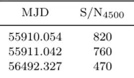
Table 1. Logbook of the HARPS polarimetric observations, in-cluding the modified Julian date of mid-exposure followed by the achieved signal-to-noise ratio.
MJD S/N4500 55910.054 820 55911.042 760 56492.327 470
the quarter-wave retarder plate relative to the beam splitter of the circular polarimeter. The reduction and calibration of archive spectra was performed using the HARPS data reduc-tion software available at the ESO headquarter in Germany, while the spectra obtained in 2013 July have been reduced using the pipeline available at the 3.6 m telescope in Chile.
To normalise the HARPS spectra to the continuum level, we used the image of the extracted echelle orders. First, we fit a continuum spline in columns of the image in cross-dispersion direction. Each column is fitted in a number of subsequent iterations until it converges to the same upper envelope of the continuum level. After each iteration, we an-alyze the residuals of the fit and make a robust estimation of the noise level based upon a statistical test of the symmetric part of the distribution. All pixels whose residuals are be-low the specified sigma clipping level are masked out from the subsequent fit. This way the smooth spline function is rejecting all spectral lines below, but leaving the continuum pixels to fit. Once all columns are processed, we fit the re-sulting smoothed curves in the dispersion direction by using the same approach with the robust noise estimation from the residuals, but this time rejecting possible outliers above and below the specified sigma clipping level. As a result, we create a bound surface with continuous first derivatives in the columns and rows. We employ a smoothing spline with adaptive optimal regularisation parameters, which se-lects the minimum of the curvature integral of the smooth-ing spline. As a test for the validity of the continuum fit, we check whether the normalised overlapping echelle orders are in good agreement with each other. The same is applied to the very broad hydrogen lines, whose wings may span over two or even three spectral orders. The typical mismatch be-tween the red and blue ends of the neighboring orders is well within the statistical noise of these orders. The usual proce-dure to normalise a series of polarimetric observations of the same target, but with different angles of the retarder, is to create a sum of the individual observations, normalise it to the continuum in the way described above, and to use the master normalised image as a template for the individual observations: by taking the ratio and fitting a regular spline to it, which then finally defines the continuum surface for the individual observations.
The Stokes I and V parameters were derived follow-ing the ratio method described by Donati et al. (1997), and null polarisation spectra were calculated by combining the subexposures in such a way that polarisation cancels out. These steps ensure that no spurious signals are present in the obtained data (e.g. Ilyin 2012). The observing logbook is presented in Table 1, where the first column gives the date of observation, followed by the S/N ratio per
resolu-tion element of the spectra in the wavelength region around 4500 ˚A.
3 MODEL PARAMETERS AND
ABUNDANCES OF HD 19400
The starting model parameters of HD 19400 were derived from Str¨omgren photometry. The observed colors (b − y) = −0.066, m1= 0.111, c1= 0.512, β = 2.708 were taken from the Hauck & Mermilliod (1998) Catalogue1. The synthetic colors were taken from the grid computed for [M/H] = 0 and microturbulent velocity ξ = 0 km sec−1 (Castelli & Kurucz 2003; Castelli & Kurucz 2006)2. Zero reddening was adopted for this star, in agreement with the results from the UVBYLIST code of Moon (1985). Observed c1and β indices were reproduced by synthetic indices for model parameters Teff = 13 868 ± 150 K and log g = 3.81 ± 0.06, where the er-rors are associated with estimated erer-rors of ±0.015 mag and ±0.005 mag for the observed c1and β indices, respectively.
The parameters from the photometry were adopted for computing an ATLAS9 model with solar abundances for all the elements and zero microturbulent velocity. Using the WIDTH code (Kurucz 2005), we derived Fe ii and Fe iii abundances from the equivalent widths of 34 Fe ii and four Fe iii lines. The equivalent widths were measured with the SPLOT task of the IRAF package using the “e” option, which integrates the intensity over the line profile. No Fe i equivalent widths were measured because the observed lines are weak and blended. The Fe ii and Fe iii abundances both satisfied the ionisation equilibrium condition and provided a good agreement between most of the observed and com-puted blended Fe i weak profiles. We did not find any trend of Fe ii abundances with the excitation potential, indicating that the adopted temperature is correct. We also did not find any trend of Fe ii abundances with equivalent widths, indi-cating that also the assumption of zero microturbulent veloc-ity is correct. For solar abundances, the model was also able to reproduce the Balmer lines, indicating that the adopted gravity is correct.
The ATLAS9 model was used to derive the abundance for all those elements that show lines in the spectrum. When-ever possible, equivalent widths were measured. For weak and blended lines and for lines that are blends of transitions belonging to the same multiplet, such as Mg ii 4481 ˚A, He i lines, and most O i lines, we derived the abundance from the line profiles. The synthetic spectrum was also used to deter-mine upper abundance limits from those lines predicted for solar abundances, but not observed.
The SYNTHE code (Kurucz 2005), together with line lists based mostly on Kurucz’s data (Castelli & Hubrig 2004; Castelli & Kurucz 2010; Kurucz 2011; Y¨uce et al. 2011) and including also data taken from the NIST database (version 5)3 were used to compute the synthetic spectrum. The syn-thetic spectrum was broadened both for a Gauss profile cor-responding to the 115 000 resolving power of the HARPS instrument and for a rotational velocity v sin i = 32 km s−1. This value was derived from the comparison of the observed
1 http://obswww.unige.ch/gcpd/gcpd.html
2 http://wwwuser.oat.ts.astro.it/castelli/colors/uvbybeta.html 3 http://www.nist.gov/pml/data/asd.cfm
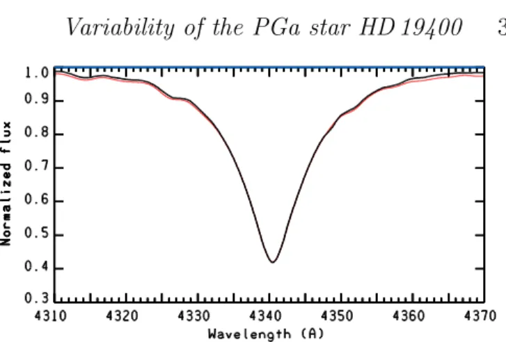
Figure 1.Comparison of the Hγ profile observed in the low-resolution FORS 1 spectrum (black) with that computed using the ATLAS12 model with parameters Teff = 13 500 K and log g = 3.9 (red in the online version).
and computed profile of several lines. We estimate an uncer-tainty of the order of 0.5 km s−1 for this choice.
Once all abundances were determined in this way, we computed an ATLAS12 model (Kurucz 2005) for the indi-vidual abundances having the same parameters as for the ATLAS9 model. However, the new ATLAS12 model did not reproduce neither the Fe ii-Fe iii equilibrium nor the hydro-gen lines. In fact, the non-solar abundances of several el-ements, and in particular the helium underabundance, al-tered the model structure in a consistent way. We therefore searched for the ATLAS12 model adequate to assure the Fe ii-Fe iii ionisation equilibrium and the Balmer lines repro-ducibility. We found that the ATLAS12 model with parame-ters Teff = 13 500 K and log g = 3.9 met these requirements. The comparison between the computed Hγ profile and the Hγ profile observed in the FORS 1 spectrum at a resolu-tion of ∼2000 on 2003 August 1 (ESO Prg. 71.D-0308(A)) is presented in Fig. 1.
The abundances log(Nelem/Ntot) of HD 19400 derived from the ATLAS12 model either from equivalent widths or line profiles are listed in Table 2, together with the solar abundances taken from Asplund et al. (2009). Similar to previous spectroscopical studies of HD 19400, no lines be-longing to the secondary were detected in the three HARPS spectra. All the lines and atomic data used for the abun-dance analysis are listed in Table A1.
The most overabundant element is Xe ([+5.22]), fol-lowed by Hg ([+4.75]), Ga ([+3.97]), P ([+2.24]), Mn ([+1.71]), Fe [(+0.73)], and Ti ([+0.67]). The elements Ne, Si, Ca, and Cr are marginally overabundant. We note that a nearly solar abundance of −4.45 dex, rather than the aver-age value of −4.37 dex derived from the equivalent widths, better reproduces with the synthetic spectrum most of the observed Si lines.
Helium is underabundant (∼ [−1.1]), but it is difficult to state a definite abundance value, because some observed profiles cannot be fitted by the computed ones, whichever is the adopted abundance. These are the lines at 4026, 4387, 4471, and 4921 ˚A. We assumed an average abundance of N(He )/Ntot= 0.007, which reproduces rather well most of the lines listed in Table A1. The wings of the lines at 4026, 4471, 5075, and 6678 ˚A are rather well reproduced by an average abundance of −2.17 dex derived from all the He i lines, but the observed core is weaker than the computed
Table 2.Abundances log(Nelem/Ntot) for HD 19400. For each element listed in the first column, we present the abundance computed using the ATLAS12 model in the second column. In parentheses is the number of lines adopted to derive the abundance for a given ion. Blended lines were counted only once. In the third column, we list the deviations from solar abundances (Asplund et al. 2009) presented in column 4. The last column gives the abundances derived by Alonso et al. (2003).
Element HD 19400 Star-Sun Sun Alonso et al. (2003)
[13500 K,3.9,ATLAS12] [13350 K,3.76,ATLAS9] He i −2.17±0.08: (14) [−1.11]: −1.05 −1.52 C ii −4.12±0.02 (4) [−0.51] −3.61 −3.52±0.28 O i −3.90 (2) [−0.55] −3.35 −3.31±0.07 Ne i −3.77±0.07 (6) [+0.34] −4.11 Na i −5.71 (2) [+0.09] −5.80 Mg ii −5.06 (4) [−0.62] −4.44 −4.65±0.30 Al ii 6−6.77 (2) 6[−1.18] −5.59 Si ii −4.36±0.17 (10) [−0.17] −4.53 −4.28±0.31 Si iii −4.37±0.02 (2) [−0.16] −4.53 P ii −4.26±0.15 (33) [+2.28] −6.63 −5.95±0.16 P iii −4.44±0.09 (4) [+2.19] −6.63 S ii −5.82 (1) [−0.90] −4.90 −5.07±0.47 Ca ii −5.50: (1) [+0.20]: −5.70 Ti ii −6.35±0.07 (9) [+0.74] −7.09 −5.69±0.37 Cr ii −6.24±0.09 (5) [+0.16] −6.40 −5.45±0.42 Mn ii −4.94±0.18 (6) [+1.67] −6.61 −4.57±0.33 Fe ii −3.79±0.14 (35) [+0.75] −4.54 −3.75±0.31 Fe iii −3.82±0.10 (4) [+0.72] −4.54 −3.67±0.30 Ni ii −5.84 (1) [−0.02] −5.82 −5.51±0.34 Ga ii −5.19±0.17 (12) [+3.81] −9.00 Sr ii −9.07 (1) [+0.10] −9.17 −6.95±0.38 Xe ii −4.65±0.17 (6) [+5.15] −9.80 Hg ii −6.16±0.13 (3) [+4.71] −10.87 −4.43
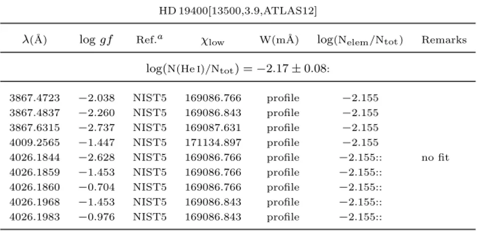
Table 3. Line by line abundances of HD 19400 from the ATLAS12 model with parameters Teff = 13 500 K, log g = 3.9. In the second and third columns, we give the oscillator strength with the corresponding data base source. The low excitation potential is listed in column 4, followed by the equivalent width and the derived abundance. For a number of lines, the abundance was derived from line profiles. The full table is available online.
HD 19400[13500,3.9,ATLAS12]
λ(˚A) log gf Ref.a χ
low W(m˚A) log(Nelem/Ntot) Remarks
log(N(Hei)/Ntot) = −2.17 ± 0.08:
3867.4723 −2.038 NIST5 169086.766 profile −2.155
3867.4837 −2.260 NIST5 169086.843 profile −2.155
3867.6315 −2.737 NIST5 169087.631 profile −2.155
4009.2565 −1.447 NIST5 171134.897 profile −2.155
4026.1844 −2.628 NIST5 169086.766 profile −2.155:: no fit
4026.1859 −1.453 NIST5 169086.766 profile −2.155::
4026.1860 −0.704 NIST5 169086.766 profile −2.155::
4026.1968 −1.453 NIST5 169086.843 profile −2.155::
4026.1983 −0.976 NIST5 169086.843 profile −2.155::
one. This kind of behaviour, common to several HgMn stars (e.g. Castelli & Hubrig 2004), is ascribed to vertical abun-dance stratification. The whole line at 4388 ˚A and the red wing of the line at 4922 ˚A can not be fitted. The cause could be due to the several blends affecting them. The other He i lines at 3867, 4009, 4121, 4713, 5015, and 5047 are well re-produced by the −2.17 dex abundance. Some of them have minor contributions of blends.
Other underabundant elements are Al (6[−1.2]), S
([−1.1]), O ([−0.69]), C ([−0.60]), and Mg ([−0.60]). Finally, Ni is marginally underabundant.
We could identify a few observed but not predicted lines as As ii. In fact, no As ii lines are included in our line list ow-ing to the lack of log gf values and excitation potentials for them. We used As ii wavelengths listed in the NIST database to identify the lines observed at 4494.30, 5497.727, 5558.09, 5651.32, and 6170.27 ˚A as due to As ii. Arsenic was
report-edly also present in the HgMn stars 46 Aql (Sadakane et al. 2001) and HD 71066 (Y¨uce et al. 2011).
No lines of rare earth elements, as well as no lines of Y ii, Pt ii, and Au ii were observed.
For comparison, the abundances from Alonso et al. (2003) are listed in the last column of Table 2. There is a large disagreement for almost all elements, except for sili-con and iron. The differences in the abundances for iron and silicon amount to 0.05 dex for Fe ii, 0.15 dex for Fe iii, and 0.06 dex for Si ii. They can be related with both the differ-ent ATLAS9 parameters and the microturbuldiffer-ent velocities adopted for the abundance analysis. The ATLAS9 parame-ters in this study are Teff = 13 870 K, log g = 3.8, [M/H] = 0.0, while those of Alonso et al. (2003) are Teff = 13 350 K, log g = 3.76, [M/H] = 0.5; the microturbulent velocities are ξ = 0.0 km sec−1 and 1.2 km sec−1, respectively. However, the differences for all the other elements are too large to be only due to the different choices for the parameters. Further-more, Alonso et al. (2003) derived abundances for numer-ous elements that we did not observe at all in our spectra, while we identified and derived abundances for Ne i, Ga ii, and Xe ii that were not mentioned at all by Alonso et al. (2003), although these elements are present with numerous lines. Unfortunately, they did not publish the list of lines and equivalent widths they used, so that any further comparison is not possible.
The ATLAS12 model was preferred to ATLAS9 for fi-nal abundance determination, to ensure consistency with the SYNTHE code in computing the line profiles; however abun-dance values derived using ATLAS9 and ATLAS12 differ by no more than 0.05 dex. The observed and synthetic spectra are presented on F. Castelli’s web page4 together with the line-by-line identification.
3.1 Emission lines
Similar to the spectral behaviour of a number of HgMn stars, the lines of multiplet 13 of Mn ii (λλ 6122-6132 ˚A) appear to be affected by emission. In fact, a very weak emission is observed for the blends λλ 6125.861, 6126.225 ˚A, while a well observable strong absorption is predicted at these wavelengths. Furthermore, the blends at λλ 6122.432, 6122.807 ˚A, at 6128.726, 6129.019, 6129.237 ˚A, and at 6130.793, 6131.011, 6131.918 ˚A are observed much weaker than computed, so that the core could have been filled by emission.
Other CP stars showing this kind of emission are, for example, 3 Centauri A (Sigut et al. 2000), (Wahlgren & Hubrig 2004), 46 Aquilae (Sigut et al. 2000), HR 6000 (Castelli & Hubrig 2007), and HD 71066 (Y¨uce et al. 2011). This phenomenon was explained ei-ther in the context of non-LTE line formation (Sigut 2001) or as due to a possible fluorescence mechanism (Wahlgren & Hubrig 2000).
3.2 Anomalous line profile shapes
In all HARPS spectra the lines of Mn ii and Hg ii present anomalous flat-bottom line profiles reminiscent of profile
4 http://wwwuser.oats.inaf.it/castelli/hd19400/hd19400.html
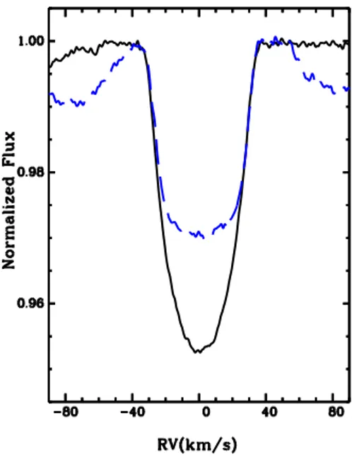
Figure 2.Comparison of the average Mn ii line profile (dashed line) with the average Fe ii line profile (solid line).
shapes observed in numerous HgMn stars (e.g., Hubrig et al. 2006a, 2011; Makaganiuk et al. 2011a), while the lines of other elements exhibit typical rotationally broadened line profiles. As an example, we display in Fig. 2 the average Mn ii profile overplotted with the average Fe ii profile, using the best almost blend-free lines of moderate strength. To construct the average Mn ii profile, we employed the Mn ii lines λλ4292.2, 4363.3, 4478.6, 4518.9, 4738.3, 4755.7, and 4764.7. Three of them, λλ4738.3, 4755.7, and 4764.7, have not been used in the abundance analysis because of their unknown hyperfine structure. We note that two more Mn ii lines, λλ4206.4 and 4365.2, were employed in the abundance analysis (see Table A1). They are not included in our sample of lines selected for the search of variability, as the line at λλ4206.4 is slightly disturbed by a blend in the blue wing and the weak line at λλ4365.2 is considerably affected by noise at the third epoch. In the calculation of the average Fe ii profile, we used the Fe ii lines λλ4122.7, 4296.6, 4491.4, 4522.6, 4923.9, 5002.0, and 5061.7, which constitute a sub-set of the sample of Fe ii lines employed in the Fe abundance determination.
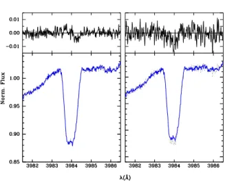
The calculation of the synthetic spectrum for individ-ual Mn ii and Hg ii lines indicates that the anomalous flat-bottom line profile shape is not caused by the presence of isotopic/hyperfine structure. In the top panel of Fig. 3, we display the synthetic profile of the Hg ii λ3984 line overplot-ted with the observed line profile. The bottom panel presents the synthetic and observed profiles of the Mn ii λ4478 line. The observed anomalous profile shape of both lines is rem-iniscent of the behaviour of line profiles of various elements in typical HgMn stars (e.g. Hubrig et al. 2006a). In spectro-scopic binaries these elements are frequently concentrated in non-uniform equatorial bands, which disappear exactly on the surface area, which is permanently facing the secondary (e.g. Hubrig et al. 2010).
Figure 3. Hg ii and Mn ii line profiles observed in the HARPSpol spectrum obtained in 2011 highlighted in black together with the synthetic profile shown by the thin red line. The shape of the line profiles belonging to Hg ii and Mn ii deviates from the purely rotationally broadened profiles observed in the Fe ii and Cr ii lines, indicating an inhomogeneous distribution of Hg and Mn on the stellar surface.
4 SPECTRAL VARIABILITY
For the study of the spectral variability we have on our dis-posal two HARPS spectra taken on two consecutive nights in 2011 December, while the third HARPS spectrum was ob-tained in 2013 July. The spectra have different quality with a S/N of about 800 for observations in 2011 and a S/N of only about 500 for the observation in 2013. To better under-stand the chemical spot pattern on the surface of HD 19400, we decided to analyse the spectral variability by compari-son of observations separated by two timescales. On the one hand we compared the spectra from 2011 with each other to study the day-to-day variations, and on the other hand, we compared the spectrum obtained in 2013 against the av-erage of the two spectra from 2011 to search for long term variation in the line profiles.
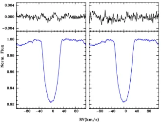
In the left panel of Fig. 4, we compare the mean Mn ii profiles obtained on two nights in 2011. In the difference spectrum the rms of the noise in the nearby continuum is about 0.05% while the variations are about 0.15%. The vari-ability of the Mn lines is detected therefore at a level of 3σ. We note that if the high-frequency noise is filtered, it becomes evident that the observed day-to-day variation is in fact four times larger than the σ of the noise of similar frequency. The year-to-year variations are apparently not
Figure 4. Profile variations of the Mn lines. Left panel: day-to-day variations; solid and dotted lines correspond to 2011 Decem-ber 15 and 16, respectively. Right panel: year-to-year variations; solid and dotted lines present 2011 and 2013 observations, respec-tively. The upper part of each panel shows the difference between the two plotted spectra.
Figure 5.Profile variations of the Fe lines. Left panel: day-to-day variations; solid and dotted lines correspond to 2011 December 15 and 16, respectively. Right panel: year-to-year variations; solid and dotted present 2011 and 2013 observations, respectively. The upper part of each panel shows the difference between the two plotted spectra.
larger than the day-to-day variations, and, since the S/N of the spectrum obtained in 2013 is lower, the variations be-tween 2011 and 2013 are not so clear. The flux differences, however, are still present at a level of about 2σ.
The same procedure as for the study of the Mn lines was applied to the Fe lines. Figure 5 shows the mean profile of the seven Fe lines. The day-to-day flux variations within the line profile are on the order of 0.13%, which is 3 times larger than the noise and of the order of 4σ, if high frequencies are filtered. Year-to-year flux differences are similar in size, but in this case represent only a level of about 1.5 times over the noise and ∼2σ, after filtering high frequencies.
To study the variability of the P ii lines, we selected the following six blend-free P ii lines: λλ4420.71, 4530.82, 4589.85, 5386.90, 6024.18, and 6043.08. The line profile dif-ference between the two spectra taken in 2011 resembles
Figure 6. Profile variations of the P lines. Left panel: day-to-day variations; solid and dotted lines correspond to 2011 December 15 and 16, respectively. Right panel: year-to-year variations; solid and dotted lines present 2011 and 2013 observations, respectively. The upper part of each panel shows the difference between the two plotted spectra.
Figure 7. Profile variations of the Ga lines. Left panel: day-to-day variations; solid and dotted lines correspond to 2011 Decem-ber 15 and 16, respectively. Right panel: year-to-year variations; solid and dotted lines present 2011 and 2013 observations, respec-tively. The upper part of each panel shows the difference between the two plotted spectra.
that of the Fe lines (Fig. 6). However, the noise in this case is higher and the detection would be only at a level of 2σ. The year-to-year comparison shows no significant variation, probably due to the rather high noise level.
The behaviour of line profiles belonging to other ele-ments with strong overabundances, in particular Hg and Ga, also indicates a non-uniform distribution. Unfortunately, for these elements, the number of useful lines is low and conse-quently the detection threshold is higher. Figure 7 shows the differences between the spectra around the only two clean Ga lines: λ4254.0 and λ4255.7. We note that the shape dif-ference in the line profiles between spectra obtained on 2011 December 15 and 16 is the same for both Ga lines. This sup-ports the genuineness of the variation behaviour, even if the flux differences are not larger than 2σ. The differences with respect to the 2013 spectrum are within the noise level.
Figure 8. Profile variations of the Hg line. Left panel: day-to-day variations; solid and dotted lines correspond to 2011 December 15 and 16, respectively. Right panel: year-to-year variations; solid and dotted lines present 2011 and 2013 observations, respectively. The upper part of each panel shows the difference between the two plotted spectra.
It is a remarkable finding that the Ga ii lines appear indicative of variability. Previous studies of He-weak mag-netic Bp stars with similar atmospheric parameters and with well established strong magnetic fields also indicated strong overabundances of P, Ga, Xe, and a few heavy el-ements, such as Pt and Hg (e.g. Collado & Lopez-Garcia 2009). Furthermore, a number of magnetic Bp stars with strongly overabundant Ga display a large variation of Ga lines, which become the strongest at longitudinal magnetic field maxima, suggesting that Ga is accumulating near the magnetic poles (e.g. Artru & Freire-Ferrero 1988). Interest-ingly, Alecian & Artru (1987) presented the radiative ac-celerations of gallium in Bp star atmospheres and concluded that the presence of a magnetic field strongly modifies the gallium accumulation.
Also the Hg line at 3984 ˚A presents noticeable variations (Fig. 8). Day-to-day variations are of the order of 0.4%, while differences of about 0.8% are present between the 2011 and 2013 observations. In both cases the variation is at a 2σ level. If high-frequencies are filtered, then the variations are at a 3−4σ level.
Due to the small number of available spectra, it is cur-rently not possible to decide whether the variability pattern of the line profiles belonging to different elements can be explained by an inhomogeneous element distribution on the stellar surface, or is due to pulsations. Although no infor-mation on the rotational period is given in the literature, its upper limit can be estimated from the measured v sin i-value and the stellar radius. Using v sin i = 32.0±0.5 km s−1 and R = 3.7 ± 0.5 R⊙ calculated using main-sequence evo-lutionary CL´ES models (Scuflaire et al. 2008), we obtain an upper limit of P 6 5.85 ± 0.8 days. It is clear that with such a rather low value for the rotation period, one can already expect to see weak variability in observations obtained on two consecutive nights.
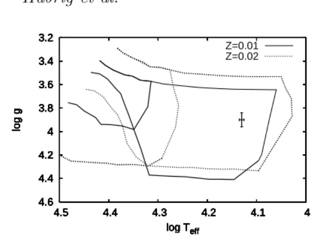
In Fig. 9 we show the position of HD 19400 in the log Teff–log g diagram. together with the boundaries of the theoretical instability strips calculated for different metal-licities (Z = 0.01 and Z = 0.02) and using the OP
3.2 3.4 3.6 3.8 4 4.2 4.4 4.6 4 4.1 4.2 4.3 4.4 4.5 log g log Teff Z=0.01 Z=0.02 3.2 3.4 3.6 3.8 4 4.2 4.4 4.6 4 4.1 4.2 4.3 4.4 4.5 log g log Teff 3.2 3.4 3.6 3.8 4 4.2 4.4 4.6 4 4.1 4.2 4.3 4.4 4.5 log g log Teff 3.2 3.4 3.6 3.8 4 4.2 4.4 4.6 4 4.1 4.2 4.3 4.4 4.5 log g log Teff 3.2 3.4 3.6 3.8 4 4.2 4.4 4.6 4 4.1 4.2 4.3 4.4 4.5 log g log Teff 3.2 3.4 3.6 3.8 4 4.2 4.4 4.6 4 4.1 4.2 4.3 4.4 4.5 log g log Teff 3.2 3.4 3.6 3.8 4 4.2 4.4 4.6 4 4.1 4.2 4.3 4.4 4.5 log g log Teff 3.2 3.4 3.6 3.8 4 4.2 4.4 4.6 4 4.1 4.2 4.3 4.4 4.5 log g log Teff 3.2 3.4 3.6 3.8 4 4.2 4.4 4.6 4 4.1 4.2 4.3 4.4 4.5 log g log Teff
Figure 9. The position of the PGa star HD 19400 in the H-R diagram. The boundaries of the theoretical instability strips for βCep and SPB stars are taken from Miglio et al. (2007) for OP opacities. Full lines correspond to strips for metallicity Z = 0.01 and dotted lines to strips with metallicity Z = 0.02.
Table 4. Previous magnetic field measurements of HD 19400 using FORS 1/2. In the first column, we list the modified Julian date of mid-exposure followed by the measurements of the mean longitudinal magnetic field hBziallusing all available spectral lines and hBzihydusing only hydrogen lines. All quoted errors are 1σ uncertainties.
MJD hBziall[G] hBzihyd[G]
52852.371 151±46 217±65
55845.295 14±24 32±26
55935.109 −65±26 −110±30
ities (http://cdsweb.u-strasbg.fr/topbase/op.html, see also Miglio et al. 2007). The PGa star HD 19400 with Teff = 13 500 K and log g = 3.90 falls well inside the classical insta-bility strip, where slowly pulsating B-type (SPB) stars are found with expected pulsation periods from several hours to a few days. Also classical magnetic Bp stars are located in the same region of the H-R diagram and frequently display strong overabundances of P, Ga, Xe, and heavy elements.
Since polarimetric observations usually consist of a number of short sub-exposures taken at different angles of the retarder wave plate, we used all available Stokes I spec-tra for each sub-exposure to search for the presence of short-term variations in Mn and Hg line profiles. During both nights in 2011 December, the time difference between indi-vidual subexposures accounts for 13 min, while it is about 20 min for the observations in 2013 July. In Fig. 10, we present the behaviour of line profiles of the Hg ii λ3984 line, and the Mn ii λ4478 line, in HARPSpol subexposures ob-tained on 2011 December 15 and 16 and on 2013 July 19. No notable line profile variations above the noise level, which is about 0.22% of the continuum flux in the 2011 spectra and about 0.32% in 2013, are detected on these time scale.
5 MAGNETIC FIELD
A few polarimetric spectra of HD 19400 were previously obtained with FORS 1 (Hubrig et al. 2006b), and most
re-Table 5.Shifts between the line centres of gravity in the right and left circularly polarised spectra obtained on three different nights. In the first column, we list the wavelengths of the Mn ii lines followed by their corresponding Land´e factors and the wavelength shifts in ˚A on each epoch.
λ geff ∆λ [˚A]
[˚A] Night 1 Night 2 Night 3
4000.033 1.076 0.0001 0.0014 4110.615 1.002 −0.0010 0.0004 4184.454 1.065 −0.0024 −0.0005 4206.367 1.362 −0.0001 0.0020 −0.0013 4240.390 0.929 −0.0046 0.0040 0.0024 4259.200 1.315 −0.0009 −0.0016 −0.0013 4260.467 2.725 −0.0027 0.0040 0.0086 4292.237 1.270 −0.0001 0.0051 4326.639 1.379 −0.0013 0.0004 0.0011 4363.255 1.112 −0.0019 −0.0005 0.0043 4365.217 1.500 −0.0042 0.0067 4478.637 1.500 −0.0104 0.0026 4518.956 1.507 −0.0007 −0.0013 4727.841 0.506 0.0031 0.0029 4730.395 0.712 0.0022 −0.0022 4734.136 0.724 −0.0010 4738.290 1.080 0.0005 4755.727 1.058 −0.0029 0.0009 4764.728 1.027 −0.0009 0.0019 0.0032 4791.782 1.085 −0.0076 −0.0042 −0.0030 4806.823 1.048 0.0013 0.0028 4839.737 1.358 −0.0031 −0.0027 0.0090
cently with FORS 2 on Antu (UT1) from 2011 May to 2012 January (Hubrig et al. 2012) at the rather low resolution of ∼2000. The magnetic field measurements from these earlier data are presented in Table 4 together with the modified Ju-lian date of mid-exposure. Out of the three measurements, weak magnetic field detections at a 3σ significance level were achieved on two different epochs. Given the low resolution of FORS 1/2, these spectra do not allow however to mea-sure the longitudinal magnetic field on lines of individual elements separately.
We note that the magnetic field topology in HgMn stars is currently unknown. The recent study of Hubrig et al. (2012) seems to indicate the existence of intriguing corre-lations between the strength of the magnetic field, abun-dance anomalies, and binary properties. Measurement re-sults for a few stars revealed that element underabundance (respectively overabundance) is observed where the polar-ity of the magnetic field is negative (respectively positive). An inhomogeneous chemical abundance distribution is ob-served most frequently on the surface of upper-main se-quence Ap/Bp stars with large-scale organised magnetic fields. The abundance distribution of certain elements in these stars is usually non-uniform and non-symmetric with respect to the rotation axis, but shows a kind of symmetry between the topology of the magnetic field and the element distribution. Assuming that a similar kind of symmetry ex-ists in HgMn and PGa stars, it appears reasonable to use the Mn ii lines for magnetic field measurements since Mn ii shows the strongest variability in the spectra of HD 19400.
The major problem in the analysis of high-resolution spectra is the proper line identification of blend free spectral
Figure 10. The behaviour of the line profiles of the Mn ii λ4478 line (left panel) and the Hg ii λ3984 line (right panel) in HARPSpol subexposures obtained on 2011 December 15 and 16, and on 2013 July 19. The overplotted profiles are presented on the top.
0 10 20 30 40 50 -9.34 10-13 λ2 geff [10-6 ] -0.010 -0.005 0.000 0.005 0.010 ∆λ [A] ˚ 0 10 20 30 40 50 -9.34 10-13 λ2 geff [10-6 ] -0.010 -0.005 0.000 0.005 0.010 ∆λ [A] ˚ 0 10 20 30 40 50 -9.34 10-13 λ2 geff [10-6 ] -0.010 -0.005 0.000 0.005 0.010 ∆λ [A] ˚
Figure 11. Linear regression analysis applied to the observations on three different nights. For each line, the shift between the line centres of gravity in the right and left circularly polarised spectra is plotted against −9.34 10−13λ2g
eff. The straight lines represent the best fit resulting from a linear regression analysis.
lines. The quality of the selection varies strongly from star to star, depending on binarity, line broadening, and the rich-ness of the spectrum. The best 22, mostly blend-free, Mn ii lines, including also six Mn ii lines used in the abundance de-termination, we employed in the diagnosis of the magnetic field on the surface of HD 19400 are presented in Table 5 together with their Land´e factors. The Land´e factors were taken from Kurucz’s list of atomic data5. As a first step, we used for the measurements the moment technique developed by Mathys (e.g. Mathys 1991). This technique allows us not only the determination of the mean longitudinal magnetic field, but also to prove the presence of crossover effect and quadratic magnetic fields. For each line, the measured shifts between the line profiles in the left- and right-hand circu-larly polarised HARPS spectra are presented in Table 5. The linear regression analysis in the ∆λ versus λ2g
eff diagram, following the formalism discussed by Mathys (1991, 1994), yields values for the mean longitudinal magnetic field hBzi between −70 G and +65 G. A weak negative longitudinal magnetic field hBzi = −70 ± 23 G at 3σ level is measured on
5 http://kurucz.cfa.harvard.edu/atoms
Table 6. Magnetic field measurements of HD 19400 using HARPS. In the first column, we list the modified Julian date of mid-exposure followed by the measurements of the mean longitu-dinal magnetic field using Mn ii lines from polarised spectra and null polarisation spectra. All quoted errors are 1σ uncertainties.
MJD hBziMn[G] hBziMn,N [G] 55910.054 −70±23 −13±24 55911.042 28±18 −18±21
56492.327 65±30 25±32
the first epoch, and hBzi = 65 ± 30 G at 2.2σ level on the third epoch.
Further, the mean longitudinal magnetic fields hBziMn,N were measured from null polarisation spectra, which are cal-culated by combining the subexposures in such a way that polarisation cancels out. The results of our measurements are presented in Table 6, and the corresponding linear re-gression plots are shown in Fig. 11. The measurements on the spectral lines of Mn ii using null spectra are labeled by
N in Table 6. Since no significant fields could be determined from null spectra, we conclude that any noticeable spurious polarisation is absent. No significant crossover and mean quadratic magnetic field have been detected on the three observing epochs.
Our assumption that the inhomogeneous distribution of Mn ii over the stellar surface is due to the action of a magnetic field does not exclude the possibility that also ions with less pronounced line profile variability are inhomoge-neously distributed across the stellar surface. Indeed, they could be concentrated towards the rotation poles, or have a predominantly symmetric distribution about the rotation axis. Among the elements showing less pronounced line pro-file variations in the spectra, the most numerous lines belong to Fe ii and P ii. Additional magnetic field measurements have been thus carried out using 35 Fe ii and 33 P ii lines listed in Table A1. Neither measurements using the Fe ii lines nor the P ii lines showed evidence for the presence of a magnetic field.
During the last few years, a number of attempts to detect mean longitudinal magnetic fields in HgMn stars have been made by several authors using the line ad-dition technique, the least-squares deconvolution (LSD; e.g. Makaganiuk et al. 2011a,b), and the multi-line Singu-lar Value Decomposition (SVD) technique (Hubrig et al. 2014). A high level of precision, from a few to tens of Gauss, is achieved through application of these techniques (Donati et al. 1997; Carroll et al. 2012), which combine hun-dreds of spectral lines of various elements. In such techniques an assumption is made that all spectral lines are identical in shape and can be described by a scaled mean profile. How-ever, the lines of different elements with different abundance distributions across the stellar surface sample the magnetic field in different manners. Combining them, as is done with such techniques, may lead to the dilution of the magnetic signal or even to its (partial) cancellation, if enhancements of different elements occur in regions of opposite magnetic polarities. A shortcoming of both techniques is that a high level of precision is achievable only if a large number of lines is involved in the analysis.
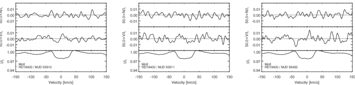
In Fig. 12, we present the results of the SVD analy-sis of the observations on all three epochs using 32 Mn ii lines selected from the VALD database (e.g., Piskunov et al. 1995; Kupka et al. 2000). We note that although the S/N of the two datasets obtained in 2011 is higher than for the most recent observation, the reconstruction for the last ob-servation was performed with a smaller number of Eigen-profiles, which results in a smaller relative noise contribu-tion. As the noise level scales with the effective dimension of the signal subspace (see Sect. 3 of Carroll et al. 2012), the noise levels of the reconstructed profiles for all three nights are approximately the same. On the first epoch, the mea-surement using the SVD technique shows the longitudinal magnetic field hBzi = −76 ± 25 G. Using the false alarm probability (FAP; Donati et al. 1992) in the region of the whole Stokes I line profile, we obtain for this measurement F AP = 0.008. According to Donati et al. (1992), an FAP smaller than 10−5 can be considered as definite detection, while 10−5 < F AP < 10−3 are considered as marginal de-tections. We note that at this epoch the Zeeman feature is well visible in the Stokes V spectrum. However, the obtained FAP value is too high for a marginal detection. The
inter-esting fact is that the observed Stokes V Zeeman feature is slightly shifted to the blue from the line center.
For the second epoch, we measure the mean longitudi-nal magnetic field hBzi = 9 ± 35 G with the corresponding FAP value of 0.045. The observed Zeeman feature in the SVD Stokes V profile is reminiscent of a typical crossover profile, and, similar to the Zeeman feature in the first epoch, is also slightly shifted to the blue from the line center. The corresponding FAP values are 0.045 for the second epoch and 0.25 for the third epoch. Especially intriguing is the ap-pearance of the SVD Stokes I profile with the corresponding Zeeman feature in the SVD Stokes V profile obtained for the third epoch. The shape of the SVD Stokes I profile shows a slight splitting shifted from the line center, indicating that we likely observe in this phase two Mn surface spots. If we assume that the Zeeman feature in the SVD Stokes V pro-file is not due to pure noise, then the observed negative and positive peaks in the Zeeman feature could probably correspond to two different Mn spots. The measured field for these features indicates a magnetic field of about −35 G for the negative peak and +35 G for the positive peak with F AP = 0.029. On the other hand, it is clear that the ampli-tude of the features inside the SVD profiles is comparable to the amplitude of the noise outside the SVD profiles.
A similar analysis using the SVD technique was carried out for 115 Fe ii and 33 P ii lines selected from the VALD database. The measurement on the first epoch using Fe ii shows a longitudinal magnetic field hBzi = −91±35 G with a false alarm probability F AP = 0.003. For the second epoch, we obtained hBzi = −28 ± 21 G with F AP = 0.009. No in-dications for a probable presence of a weak magnetic field was found on the third epoch. The obtained FAP value for the measurement on the first epoch is lower than that ob-tained for the measurement on the Mn ii lines, but is still three times too high for a marginal detection.
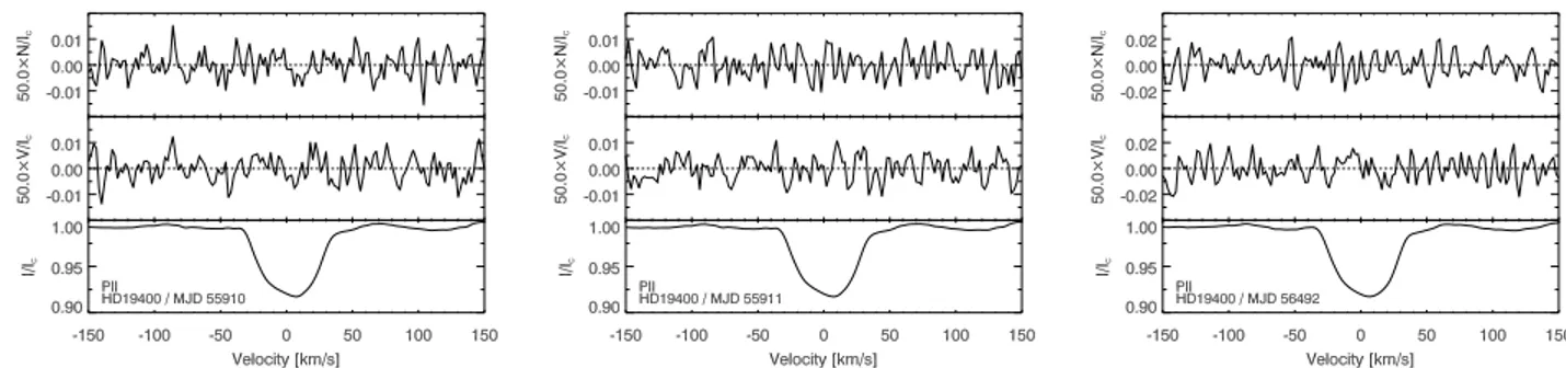
No field detection was achieved in the analysis using the P ii lines, where the Stokes V spectra appear rather flat on all three epochs. In Figs. 13 and 14, we present the results of the SVD analysis using the Fe ii and P ii lines, respectively. In summary, although some indications on the probable existence of a weak magnetic field in HD 19400 are found in our analysis, no definite conclusion on the presence of the magnetic field and its topology can currently be drawn. Obviously, more high-resolution, high S/N polarimetric ob-servations are urgently needed to properly understand the nature of this type of stars.
6 DISCUSSION
In this work, we used high quality HARPSpol spectra of the PGa star HD 19400 to carry out an abundance anal-ysis, search for spectral variability, and the presence of a weak magnetic field. We present the abundances of various elements determined using an ATLAS12 model, including the abundances of a number of elements not analysed by previous studies. We also report on the first detection of anomalous shapes of line profiles belonging to Mn and Hg. We suggest that the variability of the line profiles of certain elements is caused by a non-uniform surface distribution of these elements similar to the presence of chemical spots de-tected in HgMn stars.
Figure 12. From left to right, we present the Mn ii SVD profiles of HD 19400 obtained at the three different epochs from polarised spectra and null polarisation spectra. From bottom to top, one can see the I, V , and N profiles. The V and N profiles were expanded by a factor of 50 for better visibility.
Figure 13. From left to right, we present the Fe ii SVD profiles of HD 19400 obtained at the three different epochs from polarised spectra and null polarisation spectra. From bottom to top, one can see the I, V , and N profiles. The V and N profiles were expanded by a factor of 100 for better visibility.
One important task for future studies is to obtain de-tailed information on the pulsation behaviour of spectral lines in a few PGa stars by monitoring the behaviour of line profiles based on high quality spectroscopic time series over several hours using short exposures of the order of minutes. Current stellar models do not predict nonradial pulsations of the order of 5–20 min in mid B-type stars similar to those detected in roAp stars. On the other hand, such pulsations were not originally predicted for roAp stars either. In roAp stars, the pulsation variability is best detected in the line profiles of doubly ionised rare earth elements that build ele-ment clouds in high atmospheric layers. In close parallel to roAp stars, a theoretical consideration of B-type stars with Hg and Mn overabundances suggest that these elements can be concentrated in high-altitude clouds (above log τ = −4; e.g., Michaud et al. 1974; Alecian et al. 2011), with a poten-tial effect of weak magnetic fields on their formation (e.g. Alecian 2013). Clearly, a careful investigation of the vari-ability of mid B-type stars is of great interest to studies of stellar structure and evolution.
Our measurements of the magnetic field with the mo-ment technique using 22 Mn ii lines indicate the potential presence of a weak variable longitudinal magnetic field of the order of tens of gauss. The question of the presence of weak magnetic fields in stars with Hg and Mn over-abundances is still under debate. Bagnulo et al. (2012) used the ESO FORS 1 pipeline to reduce the full content of the FORS 1 archive, among them one polarimetric observa-tion of HD 19400 at MJD = 52852.371. While Hubrig et al. (2006b) reported for this epoch a mean longitudinal mag-netic field hBziall = 151 ± 46 G measured using the whole
spectrum and a longitudinal magnetic field hBzihyd= 217 ± 65 G using only the hydrogen lines, Bagnulo et al. (2012) measured hBziall= 124 ± 85 G, i.e. a field at a significance level of only 1.5σ. The authors state that very small instru-ment flexures, negligible in most of the instruinstru-ment applica-tions, may be responsible for some spurious magnetic field detections.
Our results using high-resolution spectropolarimetry are indicative of the potential presence of a weak magnetic field in HD 19400. Applying the moment technique to Mn lines, we measure a weak negative longitudinal magnetic field hBzi = −70 ± 23 G at 3σ level on the first epoch. At the same epoch the results from the SVD analysis of the observations using Mn ii lines show the longitudinal mag-netic field hBzi = −76 ± 25 G, and for the SVD analysis of Fe ii lines we obtain hBzi = −91 ± 35 G. However, the obtained FAP values, 0.008 and 0.003, are above the value 10−3, and thus too high for a marginal detection according to Donati et al. (1992). We note that the presented work is based on spectra obtained only at three different nights. To get a better insight into the nature of PGa stars, it is important to carry out a more complete study based on spectropolarimetric monitoring over the rotation period.
ACKNOWLEDGMENTS
We thank the referee Gautier Mathys for his useful com-ments. Based on observations made with ESO telescopes at the La Silla Paranal Observatory under programme IDs 71.D-0308(A) and 091.D-0759(A), and data obtained from
Figure 14. From left to right, we present the P ii SVD profiles of HD 19400 obtained at the three different epochs from polarised spectra and null polarisation spectra. From bottom to top, one can see the I, V , and N profiles. The V and N profiles were expanded by a factor of 50 for better visibility.
the ESO Science Archive Facility under request number MSCHOELLER51580. This work has made use of the VALD database, operated at Uppsala University, the Institute of Astronomy RAS in Moscow, and the University of Vienna.
REFERENCES
Alecian G., 2013, EAS Publ. Ser., 63, 219 Alecian G., Artru M.-C., 1987, A&A, 186, 223
Alecian G., Stift M. J., Dorfi E. A., 2011, MNRAS, 418, 986
Alonso M. S., Lopez-Garcia Z., Malaroda S., Leone F., 2003, A&A, 402, 331
Artru M.-C., Freire-Ferrero R., 1988, A&A, 203, 111 Asplund, M., Grevesse, N., Sauval, A.J., Scott, P. 2009,
Annual Review of Astronomy and Astrophysics 47, 481 Bagnulo S., Landstreet J. D., Fossati L., Kochukhov O.,
2012, A&A, 538, 129
Bilir S., Karaali S., Ak S., Yaz E., Cabrera-Lavers A., Co¸skunoˇglu K. B., 2008, MNRAS, 390, 1569
Briquet M., Korhonen H., Gonz´alez J. F., Hubrig S., Hack-man T., 2010, A&A, 511, A71
Carroll T. A., Strassmeier K. G., Rice J. B., K¨unstler A., 2012, A&A, 548, A95
Castelli F., Hubrig S., 2004, A&A, 425, 263 Castelli F., Hubrig S., 2007, A&A, 475, 1041
Castelli F., Kurucz R. L., 2003, in Piskunov N., Weiss W. W., Gray D. F., eds, Proc. IAU Symp. 210, Modelling of Stellar Atmospheres, p. 20P
Castelli F., Kurucz R. L., 2006, A&A, 454, 333 Castelli F., Kurucz R. L., 2010, A&A, 520, A57 Collado A. E., Lopez-Garcia Z., 2009, RMxAA, 45, 95 D´ıaz C. G., Gonz´alez J. F., Levato H., Grosso M., 2011,
A&A, 531, A143
Dommanget J., Nys O., 2002, Catalogue of the Compo-nents of Double and Multiple Stars (CCDM), Observa-tions et Travaux, 54, 5
Donati J.-F., Semel M., Rees D. E., 1992, A&A, 265, 669 Donati J.-F., Semel M., Carter B. D., Rees D. E., Collier
Cameron A., 1997, MNRAS, 291, 658
Drake N. A., Hubrig S., Sch¨oller M., Ilyin I., Castelli F., Pereira C. B., Gonzalez J. F., 2013, preprint (arXiv:1309.5501)
Fuhr J. R., Wiese W. L., 2006, Journal of Physical and Chemical Reference Data, 35, 1669
Hauck B., Mermilliod M., 1998, A&AS, 129, 431
Hubrig S., Mathys G., 1995, Comm. on Astroph., 18, 167 Hubrig S., Gonz´alez J. F., Savanov I., Sch¨oller M., Ageorges
N., Cowley C. R., Wolff, B., 2006a, MNRAS, 371, 1953 Hubrig S., North P., Sch¨oller M., Mathys G., 2006b,
As-tron. Nach., 327, 289
Hubrig S., et al., 2010, MNRAS, 408, L61 Hubrig S., et al., 2011, Astron. Nach., 332, 998 Hubrig S., et al., 2012, A&A, 547, A90 Hubrig S., et al., 2014, MNRAS, 440, L6 Ilyin I., 2012, Astron. Nach., 333, 213
Kling R., Schnabel R., Griesmann U., 2001, ApJS, 134, 173 Korhonen H., et al., 2013, A&A, 553, A27
Kupka F. G., Ryabchikova T. A., Piskunov N. E., Stempels H. C., Weiss W. W., 2000, Baltic Astronomy, 9, 590 Kurucz R. L., 2005, Memorie della Societa Astronomica
Italiana Supplementi, 8, 14
Kurucz R. L., 2011, Canadian Journal of Physics, 89, 417 Maitzen H. M., 1984, A&A, 138, 493
Makaganiuk V., et al., 2011a, A&A, 529, A160 Makaganiuk V., et al., 2011b, A&A, 525, A97 Mathys G., 1991, A&AS, 89, 121
Mathys G., 1994, A&AS, 108, 547
Michaud G., Reeves H., Charland Y., 1974, A&A, 37, 31 Miglio A., Montalb´an J., Dupret M.-A., 2007, Comm. in
Asteroseismology, 151, 48
Moon T. T., 1985, Commun. Univ. London Obs., 78 Nielsen K., Karlsson H., Wahlgren G. M., 2000, A&A, 363,
815
Piskunov N. E., et al. 1995, A&AS, 112, 525
Rachkovskaya T. M., Lyubimkov L. S., Rostopchin S. I., 2006, Astronomy Reports, 50, 123
Ryabchikova T. A., Smirnov Y. M., 1994, Astronomy Re-ports, 38, 70
Sadakane K., et al., 2001, PASJ, 53, 1223
Schlegel D. J., Finkbeiner D. P., Davis M., 1998, ApJ, 500, 525
Scuflaire R., Th´eado S., Montalb´an J., Miglio A., Bourge P.-O., Godart M., Thoul A., Noels A., 2008, Ap&SS, 316, 83
Sigut T. A. A., Landstreet J. D., 1990, MNRAS, 247, 611 Sigut T. A. A., Landstreet J. D., Shorlin, S. L. S., 2000,
ApJ 530, L89
Sigut T. A. A., A&A, 377, L27
Snik F., Jeffers S., Keller C., Piskunov N., Kochukhov O., Valenti J., Johns-Krull C., 2008, in Society of
Photo-Optical Instrumentation Engineers (SPIE) Conf. Ser., 7014, E22
van Leeuwen F., 2007, A&A, 474, 653
Wahlgren, G. M., Hubrig, S., 2000, A&A, 362, L13 Wahlgren, G. M., Hubrig, S., 2004, A&A 418, 1073 Y¨uce K., Castelli F., Hubrig S., 2011, A&A, 528, A37
APPENDIX A: LINE LISTS AND ABUNDANCES
Table A1. Line by line abundances of HD 19400 from the ATLAS12 model with parameters Teff = 13 500 K, log g = 3.9. In the second and third columns, we give the oscillator strength with the corresponding data base source. The low excitation potential is listed in column 4, followed by the equivalent width and the derived abundance. For a number of lines, the abundance was derived from line profiles.
HD 19400[13500,3.9,ATLAS12]
λ(˚A) log gf Ref.a χ
low W(m˚A) log(Nelem/Ntot) Remarks
log(N(Hei)/Ntot) = −2.17 ± 0.08:
3867.4723 −2.038 NIST5 169086.766 profile −2.155
3867.4837 −2.260 NIST5 169086.843 profile −2.155
3867.6315 −2.737 NIST5 169087.631 profile −2.155
4009.2565 −1.447 NIST5 171134.897 profile −2.155
4026.1844 −2.628 NIST5 169086.766 profile −2.155:: no fit
4026.1859 −1.453 NIST5 169086.766 profile −2.155:: 4026.1860 −0.704 NIST5 169086.766 profile −2.155:: 4026.1968 −1.453 NIST5 169086.843 profile −2.155:: 4026.1983 −0.976 NIST5 169086.843 profile −2.155:: 4026.3570 −1.328 NIST5 169087.831 profile −2.155:: 4120.8108 −1.723 NIST5 169086.766 profile −2.155 4120.8237 −1.945 NIST5 169086.843 profile −2.155 4120.9916 −2.422 NIST5 169087.831 profile −2.155 4143.7590 −1.201 NIST5 171134.897 profile −2.155
4387.9291 −0.887 NIST5 171134.897 profile −2.155: no fit in red wing
4437.5534 −2.015 NIST5 171134.897 profile −2.00
4471.4704 −2.211 NIST5 169086.766 profile −2.155 no fit in the core
4471.4741 −1.036 NIST5 169086.766 profile −2.155 4471.4743 −0.287 NIST5 169086.766 profile −2.155 4471.4856 −1.035 NIST5 169086.843 profile −2.155 4471.4893 −0.558 NIST5 169086.843 profile −2.155 4471.6832 −0.910 NIST5 169087.831 profile −2.155 4713.1382 −1.276 NIST5 169086.766 profile −2.155 4713.1561 −1.499 NIST5 169086.483 profile −2.155 4713.3757 −1.976 NIST5 169087.831 profile −2.155
4921.9310 −0.443 NIST5 171134.897 profile −2.301 no fit in red wing
5015.6780 −0.820 NIST5 166277.440 profile −2.155 5047.7385 −1.587 NIST5 171134.897 profile −2.155 5875.5987 −1.516 NIST5 169086.766 profile −2.301 5875.6139 −0.339 NIST5 169086.766 profile −2.301 5875.6148 +0.409 NIST5 169086.766 profile −2.301 5875.6251 −0.339 NIST5 169086.843 profile −2.301 5875.6403 +0.138 NIST5 169086.843 profile −2.301 5875.9663 −0.214 NIST5 169087.831 profile −2.301 6678.1517 +0.329 NIST5 171134.897 profile −2.301 log(N(Cii)/Ntot) = −4.12 ± 0.02
3918.968 −0.533 NIST5 131724.37 profile −4.1 blend
4267.001 +0.563 NIST5 145549.27 profile −4.1 blend
4267.261 +0.716 NIST5 145550.70 profile −4.1
4267.261 −0.584 NIST5 145550.70 profile −4.1
6578.052 −0.021 NIST5 116537.65 profile −4.15
log(N(Oi)/Ntot) = −3.9
6155.971 −1.011 NIST5 86625.757 profile −3.9
6155.989 −1.120 NIST5 86625.757 profile −3.9
6156.755 −0.899 NIST5 86627.778 profile −3.9
Table A1.Continued.
HD 19400[13500,3.9,ATLAS12]
λ(˚A) log gf Ref.a χ
low W(m˚A) log(Nelem/Ntot) Remarks
log(N(Nei)/Ntot) = −3.77 ± 0.07
5852.488 −0.455 NIST5 135888.717 14.1 −3.79 6096.163 −0.297 NIST5 134458.287 17.7 −3.85 6143.063 −0.098 NIST5 134041.840 20.9 −3.86 6266.495 −0.357 NIST5 134810.740 19.6 −3.68 6402.248 +0.345 NIST5 134041.840 36.7 −3.72 6717.043 −0.356 NIST5 135888.717 15.3 −3.70
log(N(Nai)/Ntot) = −5.71
5889.950 +0.108 NIST5 0.00 profile −5.71 blend
5895.924 −0.194 NIST5 0.00 profile −5.71 blend
log(N(Mgii)/Ntot) = −5.06
4390.572 −0.523 NIST5 80650.020 profile −5.06 blend
4390.514 −1.478 NIST5 80650.020 profile −5.06 blend
4427.994 −1.208 NIST5 80619.500 profile −5.06 blend
4481.126 +0.749 NIST5 71490.190 profile −5.06 blend
4481.150 −0.553 NIST5 71490.190 profile −5.06 blend
4481.325 +0.594 NIST5 71491.063 profile −5.06 blend
log(N(Alii)/Ntot) 6 −6.77
4663.046 −0.290 NIST5 85481.35 not obs 6−6.77 blend
5593.300 +0.410 NIST5 106920.56 not obs 6−6.77 blend
log(N(Siii)/Ntot) = −4.36 ± 0.17
3856.018 −0.406 NIST5 55325.18 123.7 −4.63
3862.595 −0.757 NIST5 55309.35 114.7 −4.42
4075.452 −1.400 NIST5 79355.02 22.6 −4.48
5688.817 +0.126 NIST5 114414.58 12.4 −4.40 blend telluric
5701.37 −0.057 NIST5 114327.15 8.7 −4.42 blend telluric
5978.93 +0.084 NIST5 81251.32 71.0 −4.52
6347.109 +0.149 NIST5 65500.47 164.7 −4.28
6371.371 −0.082 NIST5 65500.47 131.3 −4.34
6660.532 +0.162 NIST5 116978.38 15.5 −4.06
6671.840 +0.409 NIST5 117178.06 19.7 −4.09
log(N(Siiii)/Ntot) = −4.37 ± 0.02
4552.622 +0.292 NIST5 153377.050 16.7 −4.39
Table A1.Continued.
HD 19400[13500,3.9,ATLAS12]
λ(˚A) log gf Ref.a χ
low W(m˚A) log(Nelem/Ntot) Remarks
log(N(Pii)/Ntot) = −4.26 ± 0.15 4044.576 +0.669 K12 107360.25 68.5 −4.43 4420.717 −0.330 NIST5 88893.22 52.9 −4.40 4452.472 −0.083 K12 105302.37 34.0 −4.30 4463.027 +0.164 K12 105549.67 38.2 −4.46 4466.140 −0.560 NIST5 105549.67 21.1 −4.20 reversal ? 4475.270 +0.440 NIST5 105549.67 48.0 −4.51 4499.230 +0.470 NIST5 107922.93 58.0 −4.16 4530.823 +0.074 K12N 105302.37 37.0 −4.40 4554.854 −0.084 K12 106001.25 33.9 −4.20 4565.287 −0.520 NIST5 106001.25 20.9 −4.23 4581.716 −1.121 K12 101635.69 15.5 −4.01 4589.846 +0.400 NIST5 103165.61 55.2 −4.30 4602.069 +0.740 NIST5 103667.86 62.7 −4.44 4626.708 −0.320 NIST5 103339.14 29.8 −4.23
4658.309 −0.320 NIST5 103667.86 21.0 −4.49 asymm ?, uncertain laboratory wavelength?
4679.028 −0.319 K12N 106001.25 19.3 −4.45 4927.197 −0.799 K12N 103165.61 12.5 −4.33 4935.631 −0.161 NIST5 111507.66 17.6 −4.37 4943.497 +0.060 NIST5 103667.86 39.2 −4.27 5344.729 −0.280 K12N 86597.55 55.4 −4.15 5409.722 −0.390 NIST5 86743.96 60.5 −4.14 5425.880 +0.288 K12N 87124.60 103.7 −4.08 5499.697 −0.441 K12N 87124.60 49.1 −4.30 5541.139 −0.515 K12N 105302.37 16.8 −4.23 6024.178 +0.198 K12N 86743.96 106.5 −3.84 6034.039 −0.151 K12N 86597.55 73.5 −4.00 6043.084 +0.416 NIST5 87124.60 103.4 −4.07 6055.504 +0.056 NIST5 107922.93 23.9 −4.27 6087.837 −0.346 NIST5 86743.96 56.7 −4.13 6165.600 −0.341 NIST5 87124.60 49.8 −4.25 6232.297 −1.652 K12N 87124.60 7.8 −4.35 6435.282 −1.043 K12 87804.10 21.2 −4.24 6713.283 −1.257 K12 86743.96 18.8 −4.21
log(N(Piii)/Ntot) = −4.44 ± 0.09
4059.312 −0.236 K13Ph 116885.87 22.5 −4.58 4080.089 −0.494 K13Ph 116874.56 21.9 −4.35 4222.198 +0.218 K13Ph 117835.95 30.8 −4.44 4246.720 −0.120 NIST5 117835.95 23.3 −4.40 log(N(Sii)/Ntot) = −5.82 4162.665 +0.777 NIST5 128559.160 6.2 −5.82
log(N(Caii)/Ntot) = −5.50:
Table A1.Continued.
HD 19400[13500,3.9,ATLAS12]
λ(˚A) log gf Ref.a χ
low W(m˚A) log(Nelem/Ntot) Remarks
log(N(Tiii)/Ntot) = −6.35 ± 0.07
4163.644 −0.130 NIST5 20891.660 24.4 −6.28 4290.215 −0.850 NIST5 9395.710 18.8 −6.36 4294.094 −0.930 NIST5 8744.250 19.6 −6.29 4300.042 −0.442 NIST5 9518.060 31.5 −6.40 4399.765 −1.190 NIST5 9975.920 11.4 −6.27 4443.801 −0.717 NIST5 8710.440 27.1 −6.28 4501.270 −0.767 NIST5 8997.710 21.2 −6.38 4563.757 −0.690 NIST5 9850.900 18.2 −6.51 4571.971 −0.317 NIST5 12676.970 30.6 −6.37 log(N(Crii)/Ntot) = −6.24 ± 0.09 4592.049 −1.217 NIST5 32854.950 9.4 −6.21 4616.629 −1.291 NIST5 32844.760 5.9 −6.36 4618.803 −0.860 SL 32854.950 10.7 −6.25 4634.070 −0.990 SL 32844.760 8.1 −6.26 4824.127 −0.980 SL 31219.350 13.6 −6.10 log(N(Mnii)/Ntot) = −4.94 ± 0.18 4206.367 −1.553 KSG 43258.640 30.4 −4.78 hfs, weak reversal 4292.237 −1.544 KSG 43394.439 23.6 −4.99 hfs, flat core 4363.255 −2.094 K11 44899.820 15.8 −4.61 hfs, bad continuum 4365.217 −1.328 K11 53017.160 11.6 −5.12 hfs, reversal 4478.637 −0.935 K11 53597.130 21.9 −5.09 hfs, reversal 4518.956 −1.322 K11 53597.130 13.0 −5.03
log(N(Feii)/Ntot) = −3.80 ± 0.14
4122.659 −3.300 FW06 20830.553 36.4 −3.73 4258.148 −3.480 FW06 21812.045 29.9 −3.68 4273.320 −3.300 FW06 21812.045 29.7 −3.86 4286.271 −1.578 K13Fe 62171.624 18.6 −3.76 4296.566 −2.930 FW06 21812.045 45.4 −3.78 4303.170 −2.610 FW06 21812.045 60.6 −3.63 4369.400 −3.580 FW06 22409.818 24.5 −3.70 4416.819 −2.600 FW06 22409.818 51.3 −3.91 4449.611 −1.678 K13Fe 63948.803 10.3 −3.99 4489.176 −2.970 FW06 22810.346 39.9 −3.85 4491.397 −2.640 FW06 23031.283 47.9 −3.93 4507.091 −1.909 K13Fe 62689.874 11.9 −3.65 4508.280 −2.350 FW06 23031.283 62.9 −3.76 4515.333 −2.360 FW06 22939.351 65.3 −3.61 4520.218 −2.620 FW06 22637.195 52.9 −3.82 4522.628 −1.990 FW06 22939.351 69.6 −3.92 4541.516 −2.970 FW06 23031.283 43.3 −3.74 4555.887 −2.250 FW06 22810.346 63.5 −3.84 4576.333 −2.920 FW06 22939.351 40.5 −3.88 4582.830 −3.062 FW06 22939.351 34.5 −3.90 4583.829 −1.940 FW06 22637.195 85.7 −3.55 4620.513 −3.190 FW06 22810.346 22.9 −4.11
Table A1.Continued.
HD 19400[13500,3.9,ATLAS12]
λ(˚A) log gf Ref.a χ
low W(m˚A) log(Nelem/Ntot) Remarks
log(N(Feii)/Ntot) = −3.80 ± 0.14(cont.)
4629.331 −2.257 FW06 22637.195 64.6 −3.81 4635.316 −1.476 K13FeN 48039.090 46.1 −3.75 4913.296 +0.016 J07 82978.717 37.4 −3.63 4923.921 −1.206 FW06 23317.635 97.0 −3.97 4993.350 −3.680 FW06 22637.195 20.2 −3.71 5001.953 +0.933 J07 82853.704 70.2 −3.68 5018.436 −1.350 FW06 23317.635 105.2 −3.67 5030.632 +0.431 FW06 82978.717 45.5 −3.81 5061.710 +0.204 K13Fe 83136.508 39.9 −3.72 5169.028 −0.870 FW06 23317.635 104.3 −4.18 5247.956 +0.550 FW06 84938.265 47.8 −3.70 5493.831 +0.259 FW06 84685.245 33.5 −3.83 5506.199 +0.923 J07 84863.382 60.1 −3.72
log(N(Feiii)/Ntot) = −3.82 ± 0.10
4022.330 −2.040 K10 93392.300 9.3 −3.74
4371.345 −3.026 K10 66464.800 9.5 −3.86
4382.501 −2.980 K10 66523.020 12.4 −3.72
4419.596 −2.207 K10 89084.790 23.3 −3.98
log(N(Niii)/Ntot) = −5.84
4067.031 −1.847 K10Ni 32499.530 20.9 −5.84
log(N(Gaii)/Ntot) = −5.19 ± 0.17
4251.155 +0.350 RS94 113815.885 profile −4.75 hfs, blend
4254.073 −0.230 RS94 113842.301 profile −5.10 hfs
4255.720 +0.634 NKW 113842.301 profile −5.25 hfs, blend
4255.936 −0.320 NKW 113842.301 profile −5.25
4261.488 −1.100 GUES 113883.193 profile −5.15 hfs, blend
4262.014 +0.980 RS94 113883.193 profile −5.15 hfs
4263.141 −0.500 GUES 113883.193 profile −5.25 hfs
5219.658 +0.350 GUES 120550.431 profile −5.20 blend
5338.240 +0.430 RS94 118429.967 profile −5.40: bad spectrum
5360.402 +0.420 RS94 118518.461 profile −5.10 hfs, reversal ?
5363.585 +0.060 GUES 118518.461 profile −5.30 hfs, blend
5416.318 +0.640 RS94 118727.870 profile −5.20 hfs 5421.274 −0.050 NKW 118727.870 profile −5.15 hfs 6334.07 +1.000 RS94 102944.595 profile −5.40 hfs 6419.24 +0.570 RS94 102944.595 profile −5.30 hfs 6455.92 −0.080 RS94 102944.595 profile −5.30 hfs, blend log(N(Srii)/Ntot) = −9.07 4077.709 +0.148 NIST5 0.00 profile −9.07
log(N(Xeii)/Ntot) = −4.65 ± 0.17
4603.030 +0.018 NIST5 95064.38 29.1 −4.89 4844.330 +0.491 NIST5 93068.44 48.4 −4.66 5419.155 +0.215 NIST5 95064.38 37.8 −4.51 6036.170 −0.609 NIST5 95396.74 17.8 −4.55 6051.120 −0.252 NIST5 95437.67 26.0 −4.45 self-reversal ? 6097.570 −0.240 NIST5 95396.74 18.1 −4.88
Table A1.Continued.
HD 19400[13500,3.9,ATLAS12]
λ(˚A) log gf Ref.a χ
low W(m˚A) log(Nelem/Ntot) Remarks
log(N(Hgii)/Ntot) = −6.16 ± 0.13
3983.931 −1.510 NIST5 35514.624 profile −6.35
5677.102 +0.820 NIST5 105544.042 12.6 −6.07
6149.470 +0.150 NIST5 95714.406 profile −6.07 blend
a: NIST5: NIST Atomic Spectra Database, version 5 at http://physics.nist.gov/pml/data/asd.cfm;
Pii: K12: http://kurucz.harvard.edu/atoms/1501/gf1501.pos; K12N: the NIST5log gf values are replaced by the K12 values; Piii: K13Ph: http://kurucz.harvard.edu/atoms/1502/gf1502.pos;
Crii: SL: Sigut & Landstreet (1990);
Mnii: K11: Kurucz, R. L. 2011, private communication; KSG: Kling et al. (2001);
Feii: FW06: Fuhr & Wiese (2006); J07: S. Johansson (2007), priv. comm.; K10: http://kurucz.harvard.edu/atoms/2602/gf2602.pos; K13Fe: http://kurucz.harvard.edu/atoms/2601/gf2601.pos; K13FeN: the NIST5log gf values are replaced by the K13Fe values; Niii: K10Ni: http://kurucz.harvard.edu/atoms/2801/gf2801.pos;