CO-MOVEMENTS AND DYNAMIC INTERRELATIONSHIPS IN
PACIFIC BASIN STOCK MARKETS
Corhay Albert , Tourani Rad Alireza , Urbain Jean-Pierre
Abstract
In this paper, we investigate dynamic interrelationships among the stock markets of Australia, Hong Kong, Japan, New Zealand and Singapore. Using cointegration analysis and the Granger causality test we find that, although the five stock price indices share some common trends, the only stock price which does not apparently Granger cause (precede) the remaining stock prices is that of New Zealand. It is further observed that all price indices are caused by the remaining stock prices except that of Australia. With respect to the geographical separation, it appears that when we consider the Asian countries as an entity and those of the Pacific as another entity, they seem not to influence each other significantly.
Introduction
During recent years, the question of interdependence of national stock markets has attracted a lot of empirical research in the finance literature. More specifically, in the context of Pacific-Basin markets, Baily and Stulz (1990) have shown that a U.S. investor can reduce risk of his portfolio by up to 50% by investing in Pacific-Basin equities. Campbell and Hamao (1990) argue that the U.S. and Japanese markets are highly integrated though not perfectly. Results of studies by Harvey (1991) and Cho, Eun and Senbet (1986) are, however, less convincing and their evidence reveals that the Japanese and other Asian markets are not well integrated in the world markets.
The objective of this paper is to add some new evidence on the question of interdependence among Pacific-Basin countries. We investigate whether there are co-movements among the stock prices of the five largest and least restricted Pacific-Basin markets over a period of 20 years. If such co-movements are detected, it will also be important to try to assess the respective role of the countries in these "driving" forces, and more generally try to investigate the dynamic interrelationships that might exist between the different stock markets.
We are particularly concerned with the "trending behavior" of five active Pacific-Basin markets, namely those of Australia, Japan, Hong Kong, New Zealand and Singapore. We try to explore the degree to which their respective market price indices exhibit common long-term stochastic trends and the degree to which these common trends are directed by one of these market indices. For this puφose, and following previous research in this area (Corhay et al. 1992, 1993; Kasa 1992) we use the notion of cointegration (see Engle and Granger 1987). Since cointegration implies that nonstationary times series (such as stock prices) move stochastically together toward some long-run stable relationship, the existence of cointegrating relationships among various stock prices has a direct implication in terms of the existence of common trends among these series. In other words, if the random walk component behavior is a realistic hypothesis for the stock prices of these various countries, do these components differ across the national markets, or are the various markets sharing random walk components? On the other hand, cointegration also implies the existence of a Granger causal priority between the series (i.e., precedence). This framework is attractive if the purpose is to study both co-movements and dynamic relationships.
The organization of the paper is as follows: in the next section, we present the data; in the third section, we discuss the methodology and we present the empirical findings. A final section concludes the paper.
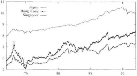
Figure 1. Logs of the Stock Price Indices
Data
In this study, we focus on the five Pacific-Basin stock markets which are the largest and have the least regulatory restrictions: Australia, Hong Kong, Japan, Singapore and New Zealand. The national stock price indices are obtained from Datastream International (a U.K.-based data service company) and are All Ordinary Shares for Australia, Hang Seng Bank for Hong Kong, Nikkei Dow Jones Average (225) for Japan, Barclays Industrial for New Zealand and Straits Times for Singapore.
Figure 2. Logs of the Stock Price Indices
The period of investigation is the same as that used in Corhay, Tourani Rad and Urbain (1994, p. 241) and covers monthly observations between February 1972-February 1992. The series were transformed into natural logs and are graphed in Figures 1 and 2.
Empirical results
Unit Roots in Stock Prices Indices
Whether stock prices are mean reverting or not is an issue which has attracted considerable empirical work over the recent years (see, for example, the often quoted study of Porteba and Summers 1988). The results reported here are intended to have some prior descriptive information on how the various national stock price indices behave during our selected sample period. No definitive conclusions on the transitory/permanent nature of stock prices will thus be made here.
As it can be observed from the figures, the various stock price indices we use in this study are likely to be well represented by I(1) processes. In order to test for the presence of stochastic nonstationarity in the data, we first investigate the integration order of our individual times series using Augmented Dickey-Fuller (1979, 1981) (ADF) tests and Phillips-Perron's (1988) non-parametrically modified Dickey-Fuller tests which allows for serial correlation and heteroscedasticity in the observed time series. In the computation of these modified statistics, we used the Newey and West (1987) non-negative long run variance estimator.
Most of our series are likely to possess some deterministic trend component or might even be characterized as trend stationary processes. Therefore, we implicitly followed the sequential testing procedure proposed by Perron (1988) which aims to start from a quite general specification with both trend and constant terms. The first hypothesis which is thus tested is that of a random walk (unit root) with drift against a trend stationary process. In the case of non-rejection, we then test for the
significance of the trend term and so on. The final hypothesis to be tested in this sequence (if all the previous less restrictive hypotheses have not been rejected) is the driftless random walk against the simple zero-mean stationary AR(1) process. The results of the unit root tests are reported in Table 1. For both ADF-type and Phillips-Perron type statistics, the lag truncation was set at four after having scrutinized the autocorrelation function of the first differences. The following notation is used: x is the usual t-test based on the following regression model without trend term and τμ is the Mest with trend term. The i = 1, 2, 3 are one sided F-type statistics respectively testing the null hypotheses of (i) (μ,
p) = (0, 1) in the model without trend, for (it) (μ, β, p) = (0, 0, 1) with trend and
(iii) (μ, β, ρ) = (μ, 0, 1) with trend.
(1)
Table 1. Unit Root Tests-Levels Test
Statistic
Japan Hong Kong Singapor e Australia New Zealand 95 percent critical value τ —1.19 -2.31 -1.04 -0.37 -0.77 -2.89 -1.59 -2.81 -2.99 -2.68 -1.52 -3.45 4.53 2.11 1.43 0.81 1.07 4.71 3.70 3.88 3.60 3.14 1.29 4.88 1.60 4.25 4.48 3.96 1.61 6.49 -0.99 -2.56 -1.14 -0.28 -0.70 -2.89 -1.78 -3.05 -2.88 -2.80 -1.57 -3.45 3.97 2.25 1.70 0.68 1.33 4.71 3.39 4.08 3.44 3.42 1.54 4.88 1.75 4.65 4.16 4.48 1.78 6.49 -1.30 -1.84 -2.31 -0.72 -1.43 -14.00 -1.17 -0.80 -1.10 -0.43 -1.02 -2.88
The "Z" versions reported in the Table 1 have the same interpretation but are computed with the Phillips-Perron non parametric correction instead of the lag augmentation.
A problem which is inherent to Dickey-Fuller based test statistics is their lack of invariance with respect to the specification of the deterministic part of the series and the fact that these deterministic terms do not have the same interpretation under the null hypothesis and the alternative. As a result, the limiting distribution changes for each deterministic specification and another table of simulated critical values is necessary. In order to overcome this problem, we also used the recently developed Schmidt-Phillips (1992) tests which is characterized by its invariance and similarity. The data generating process they consider of the usual component type where the series yt is assumed to be generated by
where εt, is assumed independently identically distributed (i.i.d.) N(0, σε2). Using this representation they derive LM tests for the null hypothesis of a unit root given by β = 1. In practice the test statistics
are computed in three steps 1. Define and construct 2. Define
3. Estimate (by OLS) the regression model
and compute the usual t statistic for = 0 (denoted by or the normalized coefficient (denoted by p) Schmidt and Phillips (1992) also relax the i.i.d. assumption in order to allow for general
dependent processes. For this purpose, we just correct the test statistic using some consistent estimator of the long run variance (Newey and West's estimator) and denote these two statistics by Zsp(p) and
. Critical values are tabulated and reported in Schmidt and Phillips (1992). As shown in Table 1 we are not able to reject the null of a unit root with drift against the trend stationary alternative hypothesis in our five series. The same battery of tests applied to the first differences confirms that our data set contains I(1) (possibly with some deterministic terms) variables.
Multivariate Cointegration
Given that our data series are well described by I(1) processes, calculating returns by differencing the series, can produce stationary processes. By using returns in the analysis, however, information about the long-run components in the price series is lost. Since our interest lies in searching for long run co-movements in stock prices, we consider the five price series jointly in order to investigate the presence of potential common trends among them.
Although most of the notions and techniques we use in this paper are now well-known in the
financial/econometric literature, we recall some of the basic tools that we are using. For more details, we refer for example to the surveys of Dolado, Jenkinson and Sosvilla-Rivero (1990). We thus focus on first order nonstationary integrated process (I(1) processes). Cointegration relationships, which allow the description of stable long-run stationary relationships among integrated variables, are then defined as (independent) linear combinations of these variables achieving stationarity. In this case, the individual series do not drift too much apart and are tied together by some long run relationship. The implications of cointegration are numerous, both from an economic and statistical point of view. In particular we know that if there are r stable long-run relationships (cointegration relations) in a k dimensional vector of time series, then these k series share k-r common stochastic trends. On the other hand, given the one-by-one relation between cointegration and the existence of Error Correction Models (see the Granger Representation Theorem in Engle and Granger 1987), then there must be some Granger Causality (i.e., precedence) in at least one direction.
In this paper, we shall exploit these relationships and investigate the presence of common stochastic trends by means of the VAR representation which has been extensively studied by Johansen (1991) and already applied to stock prices by several authors (see Corhay et al. 1992, 1993, 1994, Kasa 1992). Taking a VAR model as a starting point, Johansen (1991) and Johansen and Juselius (1990) have derived a maximum likelihood approach for both the problem of estimating and
testing the number of cointegrating relationships among the components of a k-vector x, of variables. Consider a simple VAR model for xt:
(2)
which can be reparametrized in a vector autoregressive error correction model:
(3)
Γi=-I+A1+... + Ai with i = 1,... ,p. If rank (Γp) = r < k, there are k-r unit roots in the system and r linear combinations which are stationary, that is, there are r cointegrating relationships. Γp is then written as αβ' where both a and β are (k x r) matrices of full column rank. The r first rows of β' are the r
cointegrating vectors while the elements of α are the weights of the different cointegrating vectors in the different equations. The ML estimate of a basis of the cointegrating space is given by the empirical canonical variates of xt-p with respect to Ax, corrected for the short-run dynamic and the deterministic components.1 The number of cointegrating relationships is given by the number of significant
canonical correlations. Their significance can be tested by means of a sequence of Likelihood Ratio (LR) tests whose limiting distribution is expressed in terms of vector Brownian motions (see Johansen 1988, 1991).2 Critical values have been tabulated by Johansen and Juselius (1990).
Once the number of cointegrating relationships has been determined, it is possible to test particular hypotheses concerning α and β using standard χ2 distributed LR tests. Let us now consider the five price series jointly in a Vector Error Correction Model (VECM) such as (3).3
It should directly be noted that this VECM has not only a statistical appeal. Given the presence of both first differences and levels of stock prices, this model is interpretable as explaining the joint evolution of the stock returns as functions of lagged returns as well as by the lagged level of the stock prices. Hence, if such a model is valid, it is interpretable as a multivariate statistical model for dynamic interrelationships between stock returns and stock prices.
Data analysis resulted in a final specification of the VECM consisting of allowing for an unrestricted constant in the short run in order to capture the trending behavior of the data series.4
The specification of the lag length of the VAR was tested sequentially using likelihood ratio test statistics. According to the results reported in Corhay, Tourani Rad and Urbain (1994) we chose to investigate a VAR of order 6. The computation of Johansen's trace and maximum eigenvalue test are given in Table 2, along with the estimates of the eigenvalues, normalized eigenvectors and weights. Table 2 also reports some statistics on the error processes. BJ is the usual Bera and Jarque normality test, BP is a 16th order Box-Pierce test for serial correlation, and ARCH(6) is the usual LM test for sixth order Autoregressive Conditional Het-eroskedasticity (ARCH) in the residuals.
Table 2. ML Cointegration Analysis
Statistics on the Error Processes
Countries BP(1 6)
Skewness Excess Kurtosis BJ-Normality ARCH(6)
Japan 10.03 -0.776 3.089 117.53 50.08 Hong Kong 16.17 0.594 5.233 283.122 7.20 Singapore 8.56 0.038 1.443 20.536 12.96 Australia 19.15 -0.057 0.450 2.117 6.499 New Zealand 20.25 0.326 1.135 16.847 6.263 k-6 Eigenvalues 0.132 0 0.0870 0.0560 0.033C i 0.0030
Trace Test ;f Ho Maximu m Eig envalue
0.626 r≤4 0.626
8.560 r≤3 7.934
22.159 r≤2 13.599
43.725 r≤1 21.566
77.259* r= 0 33.534* *
Normalized Cointegrating Vectors: β Matrix
Japan 1.000 0.117 3.634 0.343 0.964 Hong Kong 0.841 -0.110 -4.065 2.575 -0.682 Singapore -0.141 0.017 0.367 -5.082 -0.605 Australia -2.010 1.000 2.359 0.552 -0.981 New Zealand 0.015 -0.800 -0.979 0.759 -0.158 Weights: α Matrix Japan -0.058 -0.033 -0.003 0.003 0.001 Hong Kong -0.126 0.027 0.016 -0.005 0.002 Singapore - 0.041 0.004 0.004 0.003
0.014 Australia 0.027 -0.043 0.003 -0.002 0.002 New Zealand -0.011 0.003 -0.005 -0.007 0.002
It clearly appears that both the normality hypothesis and the absence of conditional heteroscedasticity are rejected by the data. This phenomenon often occurs with stock prices (see Kasa 1992; Corhay and Tourani Rad 1993) and should not affect our results significantly.
As shown in this table, we may not reject the hypothesis of a single cointegrating vector among our five variables (at a 95% level), a second cointegration relationship seems to occur at a 84% level, but given its graphical representation will not be considered here. The normalized coefficients are given in the first column of the β matrix. The relative magnitude of the cointegrating vector components is informative on the respective role of the countries in this financial area, in particular Singapore and New Zealand are likely to play a very minor role in the long run.
Further information can be obtained by testing explicit restrictions on the long-run parameters of the VECM, that is, restrictions on α and β. This was conducted in Corhay, Tourani Rad, and Urbain (1994) and the major results can be summarized as follows:
• Two of our five stock prices do not enter significantly into the cointegrating vector: the stock prices of Singapore and New Zealand.
• The cointegrating relationship, hence the long-run "equilibrium" relationship between the stock prices, essentially enters the equations for the three Asian markets.
This last result is directly interpretable in terms of "long run" Granger causality and tends to point out the existence of a rather integrated Pacific Basin area where the regional aspects (Asian versus Pacific Basin) have important roles to play. The presence of cointegrating relationships in the equations of a given variables implies that the latter reacts significantly to a deviation from this "long-run relation" among the various stock prices. In other words, an increase in the Japanese stock prices will in the long run affect the stock prices, and hence the returns, of the other markets.
It does not, however, tell us anything about the short run dynamic interrelationships that might exist between the markets. From (3) we effectively see that even if the cointegrating vectors do not appear in, let us say, the equation for New Zealand, dynamic links can still occur in the short run through the presence of lagged foreign returns in the equation for the New Zealand returns.
These types of dynamic interrelationships between stock markets will be investigated in the next subsection.
Granger Causality Links Among Pacific-Basin Stock Prices
To simplify the presentation, let us consider only two stock prices indices of countries 1 and 2, respectively denoted by p1t and by p2t. We consider the vector error correction model which was used in the preceding section to investigate the presence of common stochastic trends in our data set.
(4)
where the Γ matrices corresponds to the matrices of (3) and the vector (ε1t, ε2t)' is a vector of Gaussian variates with mean zero and covariance matrixΩ. In this
model, the hypothesis that the stock price p1 does not Granger cause the second stock price p2 (both in the long and short run) can be tested jointly using the following parametric restrictions (see, for example, Mosconi and Giannini 1992):
where Γ21,p is the lower left element of the matrix of long run parameters matrix Γr. If we assume cointegration among our two stock prices, then the matrix Γp is of reduced rank (here one) and can be written as αβ', that is,
(5)
investigated as two alternative potential representation of the Granger non-causality restrictions. In a recent interesting study on Granger causality in cointegrated VARs, Mosconi and Giannini (1992) studied how one could test for such restrictions and how one could estimate cointegrated VARs in this case. They propose a switching algorithm to obtain the maximized likelihood functions associated to the model under the null hypothesis of Granger non-causality. The latter can then be compared to the maximized likelihood function of the unrestricted (what concerns Granger non-causality restrictions) cointegrated VECM. As a by product,χ2 LR test statistics can be constructed with appropriate degrees of freedom. We followed this approach to study the following questions related to dynamic
interrelationships between stock markets:
• Are the individual stock price indices Granger causing the remaining countries indices (see Table 3) • Are the stock price indices of the Asian Countries Granger caused by those of the Pacific countries (see Table 3)
• Are the individual stock price indices Granger caused (i.e., preceded) by the remaining stock price indices of the other countries (see Table 4).
Table 3. Granger Non-Causality Test
Ho: "p1 does not Granger causes the stock prices of the other countries"
Country (p1) H0l:Γ21(L)=0,β1 =0 H02:Γ21(L)=0,α2=0 Japan 49.885 (χ2(21» 49.557 (χ2(24)) Hong Kong 46.281 (χ2(21)) 48.545 (χ2(24)) Singapore 41.163 (χ2(21)) 59.781 (χ2(24)) Australia 41.329(χ2(2D) 41.694 (χ2(24)) New Zealand 24.577* (χ2(21» 44.617(χ2(21))
(Japan, Hong Kong, Singapore) 56.202 (χ2(32)) 43.530* (χ2(33))
(Australia, New Zealand) 50.236 (χ2(32)) 42.559 (χ2(33))
Table 4. Granger Non-Causality Test
Ho: "p2 does not Granger causes the stock prices of the other countries"
Country (P2) H02:Γ21(L)=0,α2=0 Japan 37.804 (χ2(21)) Hong Kong 44.043 (χ2(21)) Singapore 37.443 (χ2(2D) Australia 27.253 (χ2(21)) New Zealand 39.864 (χ2(21))
The results are reported in Tables 3 and 4. We indicate in boldface the cases where we were not able to reject the null hypothesis of non-cαusαlity.
These results can be easily interpreted and point out a rather complex pattern of dynamic
interrelationships. In particular, the only stock price which does not apparently Granger cause (precede) the remaining stock prices is that of New Zealand. Contrary to what was observed in Corhay, Tourani Rad, and Urbain (1994), we see that almost all prices affect the others in some way but for the long run only. When the reverse null hypothesis is considered, we see that all price indices are caused by the remaining prices except Australia which, according to the results reported in Table 4, is apparently not caused by any of the other prices.
With respect to the geographical separation, we see that when we consider the Asian countries as an entity and those of the Pacific another entity, they seem not to influence each other significantly, although the implied significance levels are not far from the 5% boundary (respectively 0.12 and 0.08).
Conclusions
markets. Using multivariate cointegration analysis, we studied the common long-run behavior of their stock price indices over a sample period of 20 years. We found that there exists a rather integrated Pacific Basin financial area. With respect to dynamic interrelationships among these markets, the only stock price which does apparently not Granger cause (precede) the remaining stock prices is that of New Zealand. We further observe that all price indices are caused by the remaining prices except Australia. Nevertheless, with respect to the geographical separation, it appears that when we consider the Asian countries as an entity and those of the Pacific as another entity, they seem not to influence each other significantly.
Notes
1. In this presentation we have omitted deterministic components including constant, and trends for convenience.
2. Notice that the limiting distribution of these LR tests is a function of a k - r dimensional vector Brownian motion, and is not independent of the unknown deterministic components that might be present (see Johansen and Juselius 1990; Johansen 1991).
3. Part of the results reported in this subsection are taken from Corhay, Tourani Rad and Urbain (1994).
4. Notice that the potential effect of the October 1987 crash is modeled by means of a dummy variable denoted by D87 which was equal to 1 in 1987:11 to 0 elsewhere. The latter dummy only appears in the short-run dynamic of the model so that we do not allow the long-run relationships to change over time.
References
Baily, W., and R. Stulz. (1990). "Benefits of International Diversification: The Case of Pacific Basin Stock Markets." Journal of Portfolio Management Summer 761.
Campbell, J. Y., and Y. Hamao. (1990). "Predictable Stock Returns in the United States and Japan: A Study of Long-term Capital Market Integration." National Bureau of Economic Research working paper, p. 3191.
Cho, D. C, C. S. Eun, and L. W. Senbet. (1986). "International Arbitrage Pricing Theory: An Empirical Investigation." Journal of Finance 41: 313-330.
Corhay, A., and A. Tourani Rad. (1993). "Conditional Heteroscedasticity in Pacific-Basin Stock Markets Returns." Pp. 327-338 in Research in International Business and Finance: Rising Asian
Capital Markets: Empirical Studies, edited by T. Bos and T. Fetherson. Greenwich, CT: JAI Press.
Corhay, A., A. Tourani Rad, and J. P. Urbain. (1992). "GARCH and Cointegration Models for European Stock Prices." In Proceedings of Third International Trade and Finance Association
Meeting, edited by A.M. Fatemi. Texas: Laredo State University Press.
---. (1993). "Are there Common Trends in European Stock Markets?" Economic Letters 42: 385-390.
---. (1994). "Long Run Behaviour of Pacific Basin Stock Prices." Applied Financial Economics (Forthcoming).
Curnby, R. E. (1990). "Consumption Risk and International Equity Returns: Some Empirical Evidence."Journal of International Money and Finance 9: 182-192.
Dickey, D. A., and W. Fuller. (1979). "Distribution of the Estimators for Autoregressive Time Series with a Unit Root." Journal of the American Statistical Association 74: 427-431.
---. (1981). "Likelihood Ratio Test Statistics for Autoregressive Time Series with a Unit Root."
Dolado, J., T. Jenkinson, and S. Sosvilla-Rivero. (1990). "Cointegration and Unit Roots: A Survey."
Journal of Economic Surveys 4(3): 249-273.
Engle, R. R, and C. W. J. Granger. (1987). "Co-integration and Error Correction: Representation, Estimating and Testing." Econometrica 55: 251-276.
Harvey, C. R. (1991). 'The World Price of Covariance Risk." Journal of Finance 46: 111-158. Johansen, S. (1991). "Estimation and Hypothesis Testing of Cointegration in Vectors Gaussian Autoregressive Models." Econometrica 59: 1551-1580.
Johansen, S., and K. Juselius. (1990). "Maximum Likelihood Estimation and Inference on Cointegra-tion—With Applications to the Demand for Money." Oxford Bulletin of Economics and Statistics 52: 169-210.
Kasa, K. (1992). "Common Stochastic Trends in International Stock Markets." Journal of Monetary
Economics 29: 95-124.
Mosconi, R„ and C Giannini. (1992). "Non-Causality in Cointegrated Systems: Representation, Estimation and Testing." Oxford Bulletin of Economics and Statistics 54: 399-417.
Newey, W. K., and K. D. West. (1987). "A Simple Positive Definite, Heteroskedasticity and Autocorrelation Consistent Covariance Matrix." Econometrica 55: 703-708.
Perron, P. (1988). "Trends and Random Walks in Macroeconomic Time Series: Further Evidence from a New Approach." Journal of Economic Dynamic and Control 12: 297-332.
Phillips, P. C. B., and P. Perron. (1988). "Testing for a Unit Root in Time Series Regression."
Biometrika75: 335-346.
Porteba, J., and L. Summers. (1988). "Mean Reversion in Stock prices: Evidence and Implications."
Journal of Financial Economics 22: 27-59.
Schmidt, P., and P. C. B. Phillips. (1992). "Testing for a Unit Root in the Presence of Deterministic Trends." Oxford Bulletin of Economics and Statistics 54: 234-263.