Comparison of methods to model species habitat networks for decision-making in nature conservation: The case of the wildcat in southern Belgium

Journal for Nature Conservation 58 (2020) 125901

Available online 15 September 2020

1617-1381/© 2020 The Authors. Published by Elsevier GmbH. This is an open access article under the CC BY license (http://creativecommons.org/licenses/by/4.0/).

Comparison of methods to model species habitat networks for

decision-making in nature conservation: The case of the wildcat in

southern Belgium

Axel Bourdouxhe

_*

_{, R´emi Duflot}

_{, Julien Radoux}

_{, Marc Dufrˆene}

a_{Biodiversity and Landscape Unit, Gembloux Agro-Bio Tech, Universit´e de Li`ege, Gembloux, Belgium} b_{Department of Biological and Environmental Sciences, University of Jyvaskyla, Jyvaskyla, Finland} c_{School of Resource Wisdom, University of Jyvaskyla, Jyvaskyla, Finland}

d_{Earth and Life Institute, Universit´e catholique de Louvain, Louvain-la-Neuve, Belgium}

A R T I C L E I N F O Keywords:

Ecological network Habitat suitability model Least cost path

A B S T R A C T

Facing the loss of biodiversity caused by landscape fragmentation, implementation of ecological networks to connect habitats is an important biodiversity conservation issue. It is necessary to develop easily reproducible methods to identify and prioritize actions to maintain or restore ecological corridors. To date, several competing methods are used with recurrent debate on which is best and if expert-based approaches can replace data-driven models. We compared three methods: knowledge-driven (expert based), data-driven (based on species distri-bution model), and a mixed approach. We quantified their differences in habitat and corridor mapping, and prioritizations of landscape elements in terms of importance for connectivity. Key parameters generating these differences were identified. To put this into practice, the case study of the wildcat (Felis silvestris Schreber, 1777) was chosen. The results highlighted differences and similarities between approaches used. The data-driven approach was more successful in identifying the suitable habitat with regard to wildcat ecology, while the knowledge-driven approach was better able to account for obstacles to wildcat movements in the landscape matrix. However, these two methods converged for the identification of patterns of habitat patches and corridors that are important for global landscape connectivity. For both methods, we identified adjustments that can improve the outcome. The mixed approach largely differed in that it required more inputs to be performed. In the end, conservation actions were identified and could guide nature conservation practitioners in their efforts to restore landscape connectivity.

1. Introduction

Despite the establishment of protected areas, anthropogenic pres-sures on landscapes cause significant fragmentation of species habitats, increasing species extinction rates (Hanski, 2005; Stanners & Bourdeau, 1995). This is particularly the case in landscapes strongly shaped by human activities, such as Western Europe, where natural areas are reduced to small and isolated habitat remnants embedded in an anthropogenic matrix

(Jongman, Külvik, & Kristiansen, 2004; Luck, 2007). Significant fragmentation restricts population movements of species in the land-scape, limiting metapopulation functioning (Hansson, S¨oderstr¨om, & Solbreck, 1992; Jongman et al., 2004). Populations can suffer genetic drifts, including inbreeding, further increasing their extinction risk

(Hansson et al., 1992). In addition, lack of habitat connectivity prevents recolonization of potential habitats after local extinctions (Verboom, Schotman, Opdam, & Metz, 1991).

The lack of connectivity could be efficiently addressed by imple-menting ecological networks, also known as habitat networks (Melin, 1997; Opdam, Steingr¨over, & Rooij, 2006), which are progressively integrated into conservation planning (Albert et al., 2016; Rayfield, Pelletier, Dumitru, Cardille, & Gonzalez, 2016). The ambition of this conservation tool is to connect isolated populations of targeted species by linking their habitats in a coherent way and in interaction with the landscape matrix (Opdam et al., 2006). To implement ecological net-works, habitat areas or biodiversity cores and the corridors connecting them must be identified (Bennett & Mulongoy, 2006; Bernier & Th´eau, 2013; Sordello R., Billon, Amsallem, & Vanpeene, 2017; Sordello * Corresponding author at: Biodiversity and Landscape Unit, Gembloux Agro-Bio Tech, 2 Passage des D´eport´es, 5030 Gembloux, Belgium.

E-mail address: axel.bourdouxhe@uliege.be (A. Bourdouxhe).

Contents lists available at ScienceDirect

Journal for Nature Conservation

journal homepage: www.elsevier.com/locate/jnc

https://doi.org/10.1016/j.jnc.2020.125901

Romain, Billon, Amsallem, & Vanpeene, 2017). To identify them, many scientists use the concept of landscape connectivity, which can be defined as functional or structural. Functional connectivity identifies how well genes, gametes or individuals move through the landscape (Rudnick et al., 2012; Weeks, 2017). Structural connectivity measures habitat permeability to species movements based on the spatial arrangement of habitat patches, and the disturbances and other lands in the matrix (Hilty, Keeley, Merenlender, & Lidicker, 2019). This help to identify existent and potential landscapes features through which spe-cies may be able to move (Hilty et al., 2020). However, evaluation of connectivity requires spatial analyses of large and various sets of spatially explicit data that describe landscapes and the habitats corre-sponding to the natural life history traits of targeted species (Duflot, Avon, Roche, & Berg`es, 2018; Gurrutxaga, Rubio, & Saura, 2011; Sor-dello R. et al., 2017; SorSor-dello Romain et al., 2017;).

An increasingly used method to model ecological networks and support decision making regarding their implementation is based on spatial graphs theory. Spatial graphs are a simplification of landscapes where habitat patches are considered as nodes and potential movements of species as links connecting pairs of nodes (Galpern, Manseau, & Fall, 2011; Urban & Keitt, 2001; Urban, Minor, Treml, & Schick, 2009). This method allows landscape elements (habitat patches and corridors) to be prioritized for their contribution to the overall connectivity of a habitat network (Avon & Berg`es, 2016; Duflot et al., 2018; Gurrutxaga et al., 2011; Saura & Rubio, 2010). A key step is to evaluate the potential connectivity between habitat patches, which is most commonly done in current scientific literature through use of least cost paths (LCP; Sawyer, Epps, & Brashares, 2011). The landscape is interpreted as a resistance raster map representing the resistance to species movements, where each pixel has a travel cost specific to the targeted species, or group of species. Then, the path analysis identifies LCP connecting pairs of patches through the series of pixels with the lowest cumulative cost (Liu, Newell, White, & Bennett, 2018). Hence, to model spatial graph and LCPs for maintaining ecological networks, two steps must be completed: (i) identify the habitat patches to be (re)connected, and (ii) create a resistance map to describe landscape permeability to species movements.

The habitat and resistance maps used for LCP and spatial graph modeling have been defined in different ways. Some studies have built maps on the basis of expertise, using land-cover maps: some land-cover categories are considered as habitat, while every other land-cover category is assigned a resistance value according to the ecology of the targeted species (Liu et al., 2018; Watts et al., 2010). However, this method has some limitations due to the potential subjectivity of experts in identifying habitat patches and assigning resistance values to the land-cover classes (Sawyer et al., 2011; Stevenson-Holt, Watts, Bellamy, Nevin, & Ramsey, 2014). In view of the increasing use of species habitat suitability models, other studies have defined habitat patches and calculated resistance maps by transforming the map of habitat suit-ability derived from species distribution models (Duflot et al., 2018). Such data-driven approaches are expected to better reflect reality. However, this method assumes that factors influencing species move-ment behaviors are the same as those influencing the habitat suitability, which may not always be true (Zeller et al., 2018; Ziolkowska et al., 2012). Nevertheless, the use of a habitat suitability model is preferred when species observation data are available (Stevenson-Holt et al., 2014).

The emergency state of biodiversity loss pushes local stakeholders to value ecological networks as a leading strategy in nature conservation stakes (Amsallem, Deshayes, & Bonnevialle, 2010; Sordello et al., 2017). However, the lack of suitable species data often forces local nature conservation practitioners to use expert knowledge to perform ecolog-ical analyses (Stevenson-Holt et al., 2014). In this context, we compared data-driven and knowledge-driven approaches to assess if expert-based ecological network modeling could be used as an alternative solution to approaches based on habitat suitability models, when data are missing.

In this study, three approaches were compared: a “knowledge-driven method” based on expert opinion, a “data-driven method” based on a habitat suitability model, and a “mixed method” combining data and knowledge-driven methods to potentially compensate for their respec-tive weaknesses. The rationale behind the mixed approach is that a habitat suitability model is more accurate in identifying the species habitat, but may be less relevant to inform about the species movement behavior. The resistance map was therefore created following expert opinion. To align our results to the needs of nature conservation prac-titioners, our aim was to identify the differences between habitat, resistance, and priority action maps obtained by the alternative methods. We therefore focused on easily reproducible workflows based on available datasets.

To carry out this comparison, we studied the potential corridors of the wildcat (Felis silvestris Schreber, 1777) in the Walloon region (southern Belgium). The Walloon forests are the core part of a large group of forests at European scale. They play an important role for the connectivity of the species at a supra-population scale with the Alsatian and Black Forest areas. However, Belgium has one of the most frag-mented landscapes of Western Europe, reducing the connectivity of forest habitats (Jaeger, Madrinan, Soukup, Schwick, & Kienast, 2011). These issues have pushed local nature conservation stakeholders to view the wildcat and the connectivity of its habitat as a top priority. In this study, we address the following questions:

• What are the differences between the ecological network and priority action maps derived from knowledge-driven, data-driven and mixed approaches?

• Can expert knowledge lead to similar conclusions as approaches using species observation data?

• Which components generate the main differences between the different approaches tested?

2. Materials and methods

2.1. Focal species and observation data

Like other forest species, the wildcat is particularly vulnerable to historical and present fragmentation, mainly due to increased agricul-tural practices and the development of urbanized areas (Foley et al., 2005; Gibson et al., 2013). The species - once widespread in Europe - has suffered a significant decline over the past century, mainly due to the destruction of its habitat (Stahl, Artois, & Europe, 1994; Sunquist & Sunquist, 2002), but also to hunting. Its registration as a protected species has enabled the gradual recovery of its populations, but it re-mains sensitive to habitat fragmentation caused by transport infra-structure, mainly roads (Hartmann, Steyer, Kraus, Segelbacher, & Nowak, 2013; Klar et al., 2008). In addition, hybridization with do-mestic cats is a significant threat to the genetic integrity of the species (Hertwig et al., 2009; Hubbard et al., 1992; Lecis et al., 2006; Pierpaoli et al., 2003).

The wildcat is mainly a forest animal that prefers dense understory vegetation. It needs a spatial continuity of forest cover and therefore very rarely visits isolated groves (Klar et al., 2008; Libois, 1991; Libois & Mar´echal, 1994). The wildcat is also looking for undisturbed areas that are rich in prey such as small mammals. At night, the cat leaves the forest to roam the open spaces to search for prey (Klar et al., 2008; Libois, 1991; Libois & Mar´echal, 1994). The wildcat also strongly avoids village areas and isolated houses (Klar et al., 2008; Libois, 1991; Libois & Mar´echal, 1994).

For this study, we used wildcat observations (occurrence points) that combined two different databases: a field survey performed by public- service agents, and a public database built upon opportunistic obser-vations made by naturalists (Source: Obserobser-vations.be, Natagora, Natuurpunt et la Fondation "Observation International"). The former is more accurate, but the extent of the sampled area is smaller than the

area covered by opportunistic records. The latter is less accurate regarding species identification and often also less precise in terms of geographic location. To limit bias due to this dataset, we excluded opportunistic observations not confirmed by experts: only observations i) flagged with a high degree of certainty and ii) validated by an expert were retained. Observation coordinates located in an artificialized area were also relocated to the nearest neighboring ecotope (see section 2.3) which is not artificial. These observations usually result from an observer recording the observation from where he/she was and not where the animal was. While this dataset has some limitation, it is representative of the data usually available to nature conservation practitioners, which gives more pertinence to the results of this study.

2.2. Study area

The study was located in the Walloon region (southern part of Belgium) and the studied area extent was defined based on the wildcat observation range in the region. This was done to ensure that the con-structed models stay ecologically coherent, without taking into account the large diversity of ecological factors associated with different land-scape entities present in the Walloon region. To do so, a convex hull polygon was created from wildcat observations and an additional 10 km buffer (average dispersal distance of the species) was applied (Fig. 1). This buffer ensures that the wildcat habitat patches of interest are not considered in isolation from neighboring regions. This also ensures that it takes into account a recurring problem of graph analysis: the measured importance for connectivity of external habitat patches may be underestimated (Avon & Berg`es, 2016; Duflot et al., 2018; Gil-Tena et al., 2014; Saura & Pascual-Hortal, 2007). This buffer is only used to perform consistent spatial graph analyses. Therefore, comparisons

between approaches and other analyses were only performed inside the convex hull polygon. Any further mention of the study area refers to the area of data availability without the buffer.

The study area corresponds to the Ardenne plateau, representing the highest region of the country (200–700 m) and dominated by forests. The center of the study area contains a slightly undulating plateau covered by coniferous forests, with deep valleys covered by deciduous forests on its edges (CPDT, 2014). The northern and outermost southern parts of the study area lean at the bottom of the Ardenne plateau and exhibit a mixed landscape where forests give way to croplands and grasslands. The whole study area is fragmented by villages, small cities, and a dense road network, including highways; although it is less frag-mented than the rest of the country (CPDT, 2010; Quadu, Leclercq, & Hanin, 2014). The northern edge of the study area includes large town suburbs (namely Li`ege and Namur).

2.3. Environmental data layers

Land-cover and environmental maps were extracted from the eco-tope database (Radoux, Bourdouxhe, Coos, Dufrˆene, & Defourny, 2019). This database consists of a polygon map where each polygon represents an ecotope, which is considered to be the smallest ecologically distinct landscape feature (Bastian et al., 2002; Chan & Paelinckx, 2008). The ecotope map of Wallonia was obtained by segmentation and classifica-tion of a multispectral remote sensing imagery and elevaclassifica-tion model derived from LIDAR (Radoux & Bogaert, 2014). The ecotope map has 106 descriptors including land-cover variables, land-cover of the neighborhood (e.g. percentage of broad-leaved forest in a 250 m radius around the polygon and of each land-cover with 250 and 500 m radius), bioclimatic variables (e.g. rainfall of the wettest month, minimum

Fig. 1. Location of the study area delimited by data availability (blue line) and the buffer of 10 km around it (red line) in the regional context of Belgium and its neighboring countries. It covers most of the Walloon region in southern Belgium. Forest areas are represented in dark green (For interpretation of the references to colour in this figure legend, the reader is referred to the web version of this article).

temperature of the coldest month), soil variables (e.g. percentage of wet or alluvial soils), or topographic variables (e.g. mean slope of the eco-tope, azimuthal exposure). This set of 106 variables resulted from an optimization for building ecological models performed in a previous study (Delangre, Radoux, & Dufrene, 2017). (For further information about the ecotope database, visit the website: http://maps.elie.ucl.ac.be /lifewatch/ecotopes.html)

For the study, the ecotope data layer was transformed into a raster of 20 m resolution. As highways and large roads are the major obstacles for mammals (Gurrutxaga et al., 2011), and to prevent them from becoming discontinuous during the conversion to raster, a 20-meter buffer was built around these structures and was then superimposed onto the resistance maps for all methods.

This complete and precise dataset was only available for the Walloon region at the time of the study. To consistently complete the environ-mental data set in neighboring regions, a new set of patches was created, which covers the Netherlands, Luxembourg, Belgium, and neighboring parts of France and Germany. Due to this much larger area and non- availability of accurate data in every overlapping country, this expanded dataset has a lower resolution and a less complete set of environmental data. It was based on a supervised classification of Sentinel-1 (C-Band Synthetic Aperture RADAR) and Sentinel-2 (13 bands visible and infra-red sensor) images, using the ecotopes as training data. The resulting classification was consolidated based on Open Street Map data (© OpenStreetMap contributors) and the Copernicus high resolution layers. The source of elevation data was the EU-DEM from the Copernicus land monitoring service. Only factors useful to model wildcat habitat suitability were included in this dataset (see section 3).

2.4. Knowledge-driven approach

Expert-based habitat and resistance maps were derived from the land-cover classes of the ecotope database. The following land-cover classes are related to the forest environment and were considered wildcat habitats: deciduous, coniferous, and mixed forests, as well as clear-cuts including regeneration growth. A cost of resistance to move-ments between 1 for the habitat and 1000 for the most resistant land- cover was assigned based on scientific knowledge (Table 1). For other costs, we followed the order of magnitude of cost values used by Gur-rutxaga et al. (2011) for studying habitat connectivity of mammals. A

cost value of 5 was assigned to wildcat hunting territories which are open habitats with little disturbance, such as diversified grasslands and shrublands. Open habitats with disturbance such as crops were given a cost value of 60. Finally, the avoidance behavior of the wildcat towards built-up areas was taken into account by assigning the maximum cost value of 1000 to artificialized areas. The other land-cover classes also received relevant cost values according to their similarity with previ-ously mentioned ones (Table 1). In the case of the mixed approach, a resistance of 2 was assigned to land-covers corresponding to the knowledge-driven habitats that the data-driven model did not identify as optimal. Those land-covers are considered as sub-optimal habitat for the mixed approach.

2.5. Data-driven approach

We followed an adapted version of the data-driven method described in Duflot et al. (2018). MaxEnt package in R (Phillips, Anderson, & Schapire, 2006) was used to model the habitat suitability for wildcats in the study area. Opportunistic observations may lead to some bias due to the lack of true-absence data. However, precautions have been taken to diminish this bias by using Maxent model which can handle pseudo-absence. The model was built using validated observations of the wildcat as presence points, while pseudo-absences were simulated by randomly projecting points onto the study area. To prevent pseudo-absence points from being projected into areas potentially covered by wildcats, buffers with a radius of 800 m were created around points of presence in order to be excluded from the area where the pseudo-absences were projected (Klar et al., 2008). This radius corre-sponds to that of a circle whose surface area is the average area of the wildcat’s home range, which is 200 ha according to the literature (Klar et al., 2008; Libois, 1991; Sordello, 2012). The predictive variables used to train the model were extracted from the ecotope database. The set of 106 predictors was filtered to keep only variables relevant to wildcat ecology on the basis of the aforementioned literature. Then, the values of these variables were extracted for each of the presence and pseudo-absence points. Collinearity across environmental variables (or predictors) was tested (Spearman rho), and variables that were overly correlated (> 0.80) were removed to improve the quality of the model (Guisan, Thuiller, & Zimmermann, 2017). This was done manually (using “corrplot” package in R to visualize correlations) and iteratively to obtain the less correlated set of predictors. Then, the selected envi-ronmental variables were used to train the habitat suitability model, which was tested by cross-validation. The quality of the obtained model was assessed using the Area Under the Curve (AUC) and True Positive Rate (TPR), i.e., the percentage of correctly predicted presences compared to actual presence (also called sensitivity or recall). To calculate the latter, a presence/absence threshold was defined by maximizing the sensitivity and specificity (MSS) of the model as rec-ommended in the literature (Liu, White, & Newell, 2013). The obtained model was used to predict the habitat suitability over the entire studied area, using the environmental variable layer.

The habitat suitability index (HSI) map was used to determine the species habitat and define costs of movements for the non-habitat landscape matrix. The threshold selected for the calculation of TPR (MSS) was reused to determine which elements of the prediction map would be used as habitat patches for the species (Duflot et al., 2018). Thus, all pixels whose prediction probability was greater than the identified habitat/matrix threshold were considered as habitat and all others were considered as the landscape matrix. The resistance map was computed by applying a negative exponential transformation function (Eq. 1) to the HSI values of pixels not predicted as habitat (Keeley, Beier, & Gagnon, 2016):

resistance = eln(0.001)threshold×HSI_×103 (1)

where threshold is the habitat/matrix threshold and HSI is the value Table 1

Summary table of land-cover classes in the ecotope database showing the travel costs assigned to each land-cover class to create the resistance map.

Land-cover class Cost

Broad-leaved deciduous forest 1 (Habitat)/ 2 (suboptimal) Needle-leaved sempervirens forest 1 (Habitat)/ 2

(suboptimal) Needle-leaved deciduous forest 1 (Habitat)/ 2

(suboptimal)

Mixed forest 1 (Habitat)/ 2

(suboptimal) Recently cleared areas with forest regrowth, also includes

forest gaps and Christmas trees 1 (Habitat)/ 2 (suboptimal) Mixed herbaceous and tree cover (with a majority of trees) 5

Diversified grassland and shrubland 5

Shrub and herbaceous flooded 5

Mixed herbaceous and tree cover (with a majority of

herbaceous) 10

Mixed crop cover (with a minority of crops) 20 Permanent mono specific productive grassland 20 Mixed crop cover (with a majority of crops) 50

Periodically herbaceous 60

Mixture of vegetation and bare soil 60

Bare soil 500

Water 500

Densely artificialized (>50 % artificial surface) 1000 Sparsely artificialized (>25 % artificial surface) 1000

resulting from the habitat suitability model. The decay parameter of the negative exponential is set to provide resistance values ranging from 1 to 1,000.

2.6. Connectivity analysis

The habitat and resistance maps obtained by each method were then used to perform a connectivity analysis using Graphab software (Foltˆete, Clauzel, & Vuidel, 2012). Three spatial graphs were built based on (i) knowledge-driven habitat and resistance maps, (ii) data-driven habitat and resistance maps, and (iii) data-driven habitat maps and knowledge-driven resistance maps (the mixed approach). All following analyses were performed for all three approaches.

Habitat patches were further selected using a minimum surface area threshold that was set to 200 ha, which is commonly considered to be the home range area of wildcats (Klar et al., 2008; Libois, 1991; Sordello, 2012). Habitat area was used as the attribute for patches. With the use of the resistance maps, LCP analysis was performed to calculate the cost distance between neighboring patches (minimum planar graph).The cost distance was used as the attribute of links connecting pairs of habitat patches.

To build spatial graphs, we used the average dispersal distance of the wildcat, that is 10 km (Klar et al., 2008; Libois, 1991; Sordello, 2012). The dispersal distance must be multiplied by the median value of the resistance map. Thus, this distance is weighted within the reference frame used, i.e., the resistance map, and therefore is independent from the chosen scales of cost values (Avon & Berg`es, 2016; Duflot et al., 2018; Gil-Tena et al., 2014; Gurrutxaga et al., 2011). The obtained distance values, which are different in each approach because the resistance maps are different, were then used as a threshold to sort corridors that must be preserved or restored (i.e., those links with lower distance than the mean dispersal distance).

Then, the Probability of Connectivity index (PC, Eq. 2) and its par-titions were calculated to assess the importance of each habitat patch and the corridors that connect them for the overall connectivity (Saura & Pascual-Hortal, 2007). For this analysis, all links were retained (i.e., no threshold was applied). The PC index evaluates the global connec-tivity of the ecological network:

PC = ∑_n i=1 ∑_n j=1aiajp*ij A2 L (2) where n is the number of nodes (or habitat patches), aiis the attribute

characterizing node i (here patch size), aj is the attribute of node j, AL is

the total area of the study area, and p*

ij is the maximum probability

product, i.e., the maximum value of the product of the attribute of the links for all possible paths, between patch i and j (Saura & Pascual-Hortal, 2007).

Habitat patches and links were evaluated for their contribution to overall connectivity using the percentage change in PC (dPCk)when removing the element k in question (Saura & Pascual-Hortal, 2007).

dPCk=

PC − PCremove,k

PC ×100 (3)

Finally, this dPCk can be split down into three additive components:

dPCk=dPCkintra + dPCkflux + dPCkconnector (4)

where dPCk intra is the contribution of the patch or link to habitat

availability, dPCkflux is the dispersion flow in patch k from and to all

other network patches, and dPCkconnector is the contribution of the

patch or link k to the connectivity of network elements based on their topological position. The higher the connector value, the more essential the element is to the network (Saura & Rubio, 2010). dPCkconnector is

recommended to measure the importance of patches and links for the overall connectivity of a habitat network, independently of patch size

(Saura & Rubio, 2010). dPCkconnector corresponds to a part of the sum

of ai×aj×p*_ij (Eq. 2) for each pair of patches i and j in which i ∕=k, j ∕=k and k is part of the maximum probability path between them (p*

ij) (Saura

& Rubio, 2010).

The dPCkconnector values allow the creation of priority action maps

needed to maintain or increase the connectivity of the Walloon land-scape for wildcat populations (Amsallem et al., 2010; Duflot et al., 2018). Because of the generalist behavior of the wildcat regarding habitat selection, we focused mainly on corridors, but dPCkconnector

was also calculated for habitat patches. For each method, corridors (LCPs) are sorted based on dPCkconnector values to remove less

impor-tant corridors for landscape connectivity and to prioritize the remaining ones. To do so, dPCkconnector values were divided into four categories

on the basis of Jenks natural breaks (that create groups maximizing differences between groups and minimizing variance within groups). A quantitative comparison between the three resulting habitat networks has been done regarding the priority class given by dPCkconnector values

to habitat patches and corridors. The category with lowest

dPCkconnector value was then put aside in order to keep only the most

important corridors for landscape connectivity.

The remaining corridors have been categorized according to their state of conservation to differentiate corridors that must be conserved or restored. When the cumulated cost of a corridor was lower than the dispersal distance weighted to the median cost of resistance map, the corridor was considered as “conservation”, corridors were otherwise categorized as “restoration”.

Restoration actions can take several forms, such as forest patches or hedges and riparian forest restoration, to improve the landscape matrix for wildcat movements (Jerosch, Kramer-Schadt, G¨otz, & Roth, 2018). However, when a corridor must cross a road, actions to facilitate the crossing are more specific. While road infrastructure without fences are not always blocking elements compared to those with fences, some en-hancements could prevent and reduce mortality such as wildlife bridges (Hartmann et al., 2013; Klar, Herrmann, & Kramer-Schadt, 2009). Po-tential locations for such specific actions were identified by intersecting corridors considered as important to maintain overall connectivity with the road network. Roads are still important obstacles even if the corri-dors crossing them are below the weighted dispersal distance threshold, therefore both “conservation” and “restoration” corridors were included. Restoration corridors that do not cross roads were put into a “non-suitable habitat” category if no obstacles could be identified.

In order to quantitatively measure if priority conflicts with roads were located at the same places, we used a Jaccard similarity index. To do so, a buffer of 5 km was calculated around intersections between priority corridors and roads. Then, the area of intersection between those buffers from the two compared approaches was calculated and divided by the total area of buffers of the two approaches. This was done between all three approaches. A higher value explains a higher simi-larity in terms of location between identified conflicts with roads. This value of 5 km was arbitrarily chosen as a compromise between study extent, the precision needed for corridor spatial location, and a sensi-tivity analysis performed to find the best value to highlight similarities and differences. The study extent plays a role in the potential conver-gences of buffers and the precision should not be too excessive because precise location of corridor restoration actions should also align with actual land-use planning opportunities.

A selection based on the different priority categories was made to study the variation in the Jaccard index while taking into account i) all conflict points, ii) conflict points of first and second priority, and iii) conflict points of first priority only.

3. Results

3.1. Wildcat habitat maps

After refining the wildcat observation data, there were 1319 pres-ence points available, and as many pseudo-abspres-ences were generated to calibrate the MaxEnt model. Among presences, 40 points located in artificial areas were relocated to avoid any unintended effect on the model. The obtained model has satisfactory accuracy with an AUC of 0.79 and a TPR of 0.75. The presence/absence threshold that maximizes the sensitivity and specificity of the model is 0.56. Pixels with Habitat Suitability Index above this value were considered as potential habitats of the wild cat, representing 35.9 % of the study area. As a comparison, the area considered as habitat in the knowledge driven approach rep-resented 56.4 % of the study area. However, the TPR calculated for this approach reaches 0.47 which is 0.28 lower than data-driven approach. Maps of the suitable habitat obtained by the two approaches can be found in Appendix A (in Supplementary material). Concerning the data- driven approach, the main factors influencing habitat suitability for the wildcat were contextual variables. For instance, the most important factor was the presence of forests dominated by coniferous trees within a 250 m radius, which is positively correlated to the habitat suitability. The second most important factor was the presence of artificial light in the neighborhood, which is negatively correlated to the habitat suit-ability and positively correlated to the presence of artificial areas. The list of variables retained in the final model and their relative importance in predicting habitat suitability can be found in Appendix B (in Sup-plementary material).

3.2. Resistance maps

The two resistance maps created following data-driven and knowledge-driven approaches are available in Appendix C (in Supple-mentary material). To help in comparing those results, we calculated the absolute difference of costs between the two approaches for each land- cover category (Fig. 2). Land-cover were grouped in a broader cate-gory if they share similar costs for both approaches. Forest environment land-covers can be related to the habitat of the species and generally have a mean difference close to zero but a large variance. Land-covers related to artificialized areas also had a mean difference near zero and an even larger variance. Those land-covers are generally well identified

as habitat or blocking elements but differences still exist, as shown by large variances. In contrast, important differences exist between the two resistance maps for other land-covers, particularly water bodies and bare soils with a mean difference higher than 100, while crop and productive pastures showed differences near 100 in absolute difference of resistance values. Bare soils represent only 0.06 % of the study area and were not taken into account in the model of the data-driven model which explain the important difference of cost. Yet, their sporadic location should diminish their impact on connectivity. In contrast, water bodies such as rivers are linear elements which have a potential role of blocking elements. Crop and pastures occupy larger areas. Therefore, differences of cost for these two land-cover should have a strong influ-ence on the connectivity results. Differinflu-ences measured can be explained by their location near forests or cities and the use of contextual variables in the data-driven approach. A high cost is given in the surrounding areas of cities, villages, and roads, whereas the opposite applies to water bodies, crops, and pastures near forests, i.e., a lower resistance due to proximity to forest. This proximity effect was not considered in the knowledge-driven approach. As a consequence, rivers are less well identified as blocking elements in the data-driven approach, particularly in forest environments. However, crop and pastures near forests can contribute to corridors and can be identified as more favourable element for species movement with this approach. Proximity variables also affected land-cover related to forest environments (when forest was part of the landscape matrix) explaining some of the differences. In the data- driven resistance map, forests located in artificial landscapes are less favorable for wildcat connectivity. This influence of local context does not emerge from the knowledge-driven method because ecotope poly-gons are considered independently from each other. For instance, the mean percentage of presence of artificialized areas in a 500 m radius around each ecotope identified as habitat of the species has been calculated. This mean percentage is 0.9 % for the knowledge-driven approach and 0.4 % for the data-driven one. This result indicates that more knowledge-driven habitat patches are surrounded by artificialized areas than data-driven ones. This converges with our hypothesis that proximity to artificialized areas impacts forest habitat suitability in the data-driven approach and not in the knowledge-driven one.

The median values of resistance per meter traveled for the expert- based, data-based, and mixed methods are 40, 5, and 2 (cost/meter) respectively. The resulting weighted dispersal distances for each method are 20,000, 2,500, and 1000 (in cost units).

3.3. Connectivity analysis

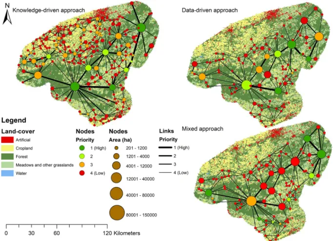
To visualize priority corridors, a schematization of habitat patches and corridors was performed, using the graph representation, i.e., nodes and links (Fig. 3). Gaps between forest patches would not be visible on a land-cover map at the regional scale. Because Fig. 3 stays complex despite the schematization, it was not possible to highlight the cumu-lated cost of each corridor. This useful information, that makes it possible to quickly visualize actual connectivity between patches, is available in Appendix D (in Supplementary material). We compared the three resulting habitat network regarding the priority class given by

dPCkconnector values to habitat patches and corridors (Table 2). As a

reminder, the lowest priority class entities (priority 4) are not consid-ered important for connectivity in further analysis. For each approach and each priority class, habitat area in hectares and number of corridors were calculated. We can see that for all three approaches tested,

dPCkconnector identified a few main patches and corridors needed to

maintain connectivity in the network. The data-driven is the approach that identified the most first priority corridors (3). Besides, big habitat patches are often considered as important for the connectivity which increase habitat area of importance except for the mixed approach. The knowledge-driven and the data-driven approaches both identified large and central patches along the Ardennes as the most important patches for connectivity. The mixed approach showed a different result with Fig. 2. Boxplots of absolute costs differences between resistance maps from

knowledge and data-driven approaches, for each land-cover class. A log 10 transformation has been applied to the y axis while land-cover categories are arranged from least to highest resistance (left to right).

large external patches marked as important. It is crucial to note that all approaches also identified small patches as important for connectivity, particularly the data-driven and the mixed approaches. For the mixed approach, three patches in the southern part of study area were classi-fied in the top two categories of priority. All three methods identiclassi-fied several important corridors following the Ardenne high plateau sum-mits. Those central corridors were also generally those with the highest cumulated cost for all methods (Appendix D (in Supplementary mate-rial)). The knowledge-driven approach identifies about twice as many corridors (248) than the other methods (Table 2). This approach high-lighted an important path in southern Ardennes (southwest of the study area), which was not shown by other approaches. It also identified corridors connecting central patches with southernmost ones and also

with south-eastern patches. In general, the knowledge-driven approach identified a much more connected landscape.

For the knowledge-driven approach, 49 out of 248 corridors were considered as important for connectivity based on their dPCkconnector.

Those 49 corridors were all considered for conservation objectives as their cost did not exceed the weighted dispersal distance. Concerning conflict with obstacles, 19 were related to roads. The others were not related to a lack of suitable habitat because their cost did not exceed the weighted dispersal distance.

Concerning the data-driven approach, 10 out of 125 corridors were considered important for connectivity and all of them had conservation goals. 6 of them were related to road conflict.

In the case of the mixed approach, 11 out of 124 corridors were important for connectivity. 4 of them had conservation goals, while 6 had restoration and 7 had road conflict.

This sorting helped to build priority action maps that show, for each method, habitat patches, corridors that must be preserved (important conservation corridors), and road conflicts (intersection between important corridors of conservation or restoration and major road net-works). Due to high values of weighted dispersal distance, no corridors with a lack of suitable habitat were identified (restoration corridors not crossed by a road).

The different priority action maps showed that the corridors needing restoration to improve overall connectivity are small corridors crossing important road infrastructure such highways or 2 × 2 lane national roads (Fig. 4). These roads split important forest areas from north to south. Knowledge-based priority action maps identified more obstacles in accordance with the higher number of corridors in that map.

Table 3 shows the different values of the Jaccard index measuring Fig. 3. Schematic representation of the connectivity of habitat patches for each approach, overlaid on land-cover map. Habitat patches are represented by nodes whose size is proportional to their area, the different colors represent the respective importance of each patch for the connectivity based on the dPC Connector calculation. Corridors are represented by links, the thicker they are the more important they are to support global connectivity.

Table 2

Habitat area and number of corridors are compared across the three approaches tested according to their importance to maintain connectivity. Priority classes were created using Jenks natural breaks on dPCkconnector values ranking them

from lowest (Priority 4) to highest priority (Priority 1).

Priority 4 Priority 3 Priority 2 Priority 1 Sum Habitat area (km2₎ Knowledge-driven 864 1357 668 2567 5456 Data-driven 801 885 1081 703 3470 Mixed 1647 813 138 872 3470 Number of corridors Knowledge-driven 199 44 4 1 248 Data-driven 115 6 1 3 125 Mixed 113 7 3 1 124

location proximity of corridors in conflict with roads between the three approaches. We can see that the mixed and data-driven approaches share the most similarities but few are shared with the knowledge- driven approach. However, the similarity between the knowledge- driven approach and the two others doubles when we focus on high priority conflicts. With first priority conflicts, this similarity approaches 50 %.

4. Discussion

4.1. Modeling habitat and resistance maps

The different methods used to model the habitat network of the wildcat led to different results. First, there were important differences in identification of suitable habitat patches. Despite a much larger area was predicted as habitat in the knowledge driven approach (1.5 times larger), the habitats mapped by the data-driven approach included 28 % more of total observations, suggesting a better identification of habitat suitability. The knowledge-driven map shows its limitations by only considering the local land-cover. In contrast, the data-driven approach accounted for local characteristic and surrounding context, which is closer to wildcat ecology. It does not come close to villages and human- related land-cover types and prefers proximity with forests, particularly the ecotone between forests and open natural areas to hunt (Klar et al., 2008). Accordingly, the final habitat suitability model included contextual variables such as presence of needle-leaved forest in a 250 m radius and artificial light. The knowledge-driven approach did not use contextual variables, so the quality of the identified habitat patches can be questioned as there are more of them in densely populated areas than in the data-driven approach. Contextual variables such as proximity to built-up areas or forests could also be considered in the knowledge-driven approach, but would be much more difficult to parameterize (i.e., define proximity distance) and would require addi-tional time-consuming GIS (Geographic Information System) data ma-nipulations. The resulting networks are therefore very different. The Fig. 4. Action maps identifying obstacles and important corridors that need to be taken into account to improve general connectivity of the Walloon landscape. Priority obstacles include conflicts with conservation and restoration corridors crossing a road (represented by black crosses). “Corridors to be maintained” cor-responds to all important corridors for connectivity with conservation goals, they are represented by green triangles (For interpretation of the references to colour in this figure legend, the reader is referred to the web version of this article).

Table 3

Results of Jaccard index analysis performed on priority conflict between corri-dors and roads based on priority action maps. Values range from 0 to 1, higher values indicate that conflict points are closely located to each other.

habitat map resulting from the data-driven approach may be considered conservative and focused on higher quality patches. However, the generalist behavior of the wildcat makes it difficult to map its suitable habitat, hence the intermediate predictive accuracy of the habitat suit-ability model (AUC = 0.79). It is known that wide-ranging species pro-duce models with a lower accuracy than habitat-specific ones (Segurado & Araújo, 2004). However, modeling the habitat suitability of the wildcat is also sensitive to calibration data. The observation data used here is not optimal and may represent biased reality, and contains less information than presence-absence data. Radio-tracked data could be used as relevant data to create very performant resistance maps, with more realistic information related to movements, but there is a recog-nized shortage of such data (Eycott et al., 2012). Approaches based on expert opinion and opportunistic observation data are therefore most often used (Stevenson-Holt et al., 2014). It remains important to stress that the effectiveness of either method compared in this study may depend on the data available, the species considered, and on the land-scape in which the study is carried out (McClure, Hansen, & Inman, 2016). In our case, the obtained model represents the probability of seeing the wildcat rather than identifying its current habitat. It is thus important to take those limitations into consideration when designing a conservation action plan from such a method.

Second, the resistance maps obtained from the two approaches were partially divergent. However, forest and densely populated areas were still distinctly identified in both maps (Appendix C (in Supplementary material)). The main differences were due to smoother transitions be-tween habitat and matrix in the data-driven approach, as a result of contextual variables, and leading to huge differences in costs for areas near forests and artificial areas (Fig. 2). The huge variance within land- covers corresponding to blocking elements suggests that the data-driven approach did not correctly identify obstacles as such. This could be explained by a high proportion of forest land-cover decreasing the cost

value of surrounding obstacles such as rivers or roads crossing forests. It is therefore sometimes difficult to handle the effect of contextual vari-ables because it does not always give the results sought. This problem may be avoided in the mixed method by using the knowledge-driven resistance map. However, in that approach, assigning cost values to land-covers other than obvious obstacles remains subjective, or even speculative. Also, in this approach, the use of local context variables, although possible, remains even more questionable. As a compromise, the data-driven method could be combined with manually defined costs for certain obstacle elements, herein roads (Stevenson-Holt et al., 2014). However, this would require case-specific adaptations, which may be too time consuming to be performed on a regular basis.

4.2. Connectivity analysis

Connectivity analysis through use of dPCkconnector allowed

priori-tization of elements that are important to maintain overall connectivity. All approaches located these elements between the large forest patches along the Ardennes plateau (Fig. 3). Additional smaller habitat patches and connections located in the southern part were also identified as important. The data-driven approach prioritized a lower area of habitat patches and fewer corridors, which can help to reduce the number of priority actions when resources available for conservation are limited.

In general, the dPCkconnector values for patches and corridors were

low, showing a relative weak effect of fragmentation in the study region. Nevertheless, road infrastructures still have a negative impact on the wildcat population (Hartmann et al., 2013; Klar et al., 2008), and their effect on connectivity may have been compensated here by the high dispersal capacity of the wildcat, its generalist behavior, and relatively high habitat availability. Furthermore, the study area is one of the less fragmented regions of Belgium (Quadu et al., 2014). The use of

dPCkconnector values is therefore best suited for relative comparisons

between elements of the network.

The differences in the dPCkconnector range of values across

ap-proaches resulted from the use of different habitat and resistance maps.

dPCkconnector calculations were also based on the dispersion distance

derived from the dispersal capacity of the wildcat adjusted by the me-dian cost value of resistance maps. These meme-dian cost values were different across the three approaches. The lowest median travel cost value was in the mixed approach (2/meter), indicating a more perme-able matrix. This was probably due to suboptimal habitats, which were excluded from favorable habitat patches in the data-driven habitat map, but considered permeable (low costs) in the knowledge-driven resis-tance map. In addition, habitat patches from the data-driven approach overlap areas considered as less favorable in the knowledge-driven one (reducing areas with higher costs in the mixed approach).

Calculating the weighted dispersal distance using the median cost value allows comparisons to be made between the cumulated cost of LCP and the dispersal distance of the focal species, independently from the scale of cost allocated to the landscape (Avon & Berg`es, 2016; Duflot et al., 2018; Gil-Tena et al., 2014). However, comparing different ap-proaches highlights, again, the fact that weighted dispersal distances and related dPCkconnector values are useful for relative comparisons (e.

g. ranking/prioritization) within one particular map/approach, but may

have limited relevance out of their context. Therefore, we advise to limit the use of dPCkconnector values to the comparison of element

impor-tance within the same approach and not between different methods. Instead, priority ranks should be used for comparison.

4.3. From connectivity analysis to conservation actions

Despite large differences, the most important conflict points between high priority corridors and roads were similarly identified across the different approaches (Fig. 5). These high priority conflicts can be considered with certainty as priority areas for conservation and used to guide nature conservation practitioners in their efforts to restore land-scape connectivity. Therefore, the knowledge-driven approach still identified similar high priority conflicts and this approach should not be totally excluded when qualitative datasets are missing. However, many important corridors that must be preserved differ significantly between approaches. The data-driven and mixed approach share the most simi-larities with regard to the locations of the conflict points compared with knowledge-driven one. This is probably because data-driven and mixed approaches share the same habitat patches while knowledge-driven identified habitat patches in other areas. Corridors have therefore more chance to be in similar places. But difference still exists between data-driven and mixed approach due to the use of different resistance map. Differences in location of priority action between approaches can be, at least in part, explained by the dispersal distance weighted by the median cost value of the resistance map. Those weighted dispersal dis-tances influenced the categorization of corridors as “conservation” or “restoration” sites and the way obstacles were identified as blocking elements or not. Therefore, those categories may be seen as indications for practitioners, but do not directly infer the probability of movement through them.

Nature conservation practitioners should bear in mind that quanti-tative comparison of priority action maps remains difficult because of the spatial aspect. We propose in this study the use of a Jaccard simi-larity index. Although the method has its own limitations due to arbi-trary choices made, the results were useful and relevant. We therefore advise the use of such a quantitative comparison method. Also, some arbitrary choices have been made following the up to date knowledge (e.

g. dispersal distance, resistance scales, connectivity metrics), with

po-tential consequences on the results.

5. Conclusion

Our study tested different approaches to habitat network modeling

from habitat and resistance maps to the creation of priority action maps. It comes out that core habitats and corridors are confirmed, but that only the data-driven method could take advantage of the multiple impacts of contextual information on the final results. Although we do not have access to the true use of space by the wildcat, the comparison of the results therefore seems to indicate the data-driven approach correspond best to the known ecology of the species. Moreover this approach can be improved by systematically identifying obstacles based on expert opinion. The knowledge-based method could be more competitive with additionnal parameters in case of absence of observation, but a robust and systematic method to gather expert opinion is needed as well as in- depth sensitivity analysis. In the end, the data-driven approach with presence-only data was more efficient in this study. However, all ap-proaches identified the same important corridors, showing the impor-tance of maintaining the continuity of the Ardennes plateau. The graph analysis of the mixed approach did not highlight central patches important for landscape connectivity. Also, this method requires more inputs (gathering expert opinion and performing habitat suitability models) for less accurate results. The study shows some limitations as arbitrary choices were made throughout, but precautions were taken and discussed. We highlight that one important parameter is the weighted dispersal distance. We suggest therefore that the graph-based metrics should be used for prioritizing connectivity of landscape ele-ments, rather than the direct use of LCP values. We also encourage using sensitivity analysis of dispersal distance to detect uncertainty associated with this parameter. In the end, the different priority action maps, albeit different, identified similar conflict points between important corridors and roads. Those conflict points could guide nature conservation prac-titioners in their efforts to improve landscape connectivity.

Funding

This work was supported by F´ed´eration Wallonie-Bruxelles in the frame of the Lifewatch-WB project.

Declaration of Competing Interest

The authors report no declarations of interest.

Acknowledgments

The authors would like to thank the DEMNA (D´epartement de l’´Etude du Milieu Naturel et Agricole) and Natagora for sharing their data. They also thank WWF Belgium and particularly Corentin Rousseau for participating in the development of the research question. RD is a postdoctoral fellow of the Kone Foundation.

Appendix A. Supplementary data

Supplementary material related to this article can be found, in the online version, at doi:https://doi.org/10.1016/j.jnc.2020.125901.

References

Albert, C., Galler, C., Hermes, J., Neuendorf, F., von Haaren, C., & Lovett, A. (2016). Applying ecosystem services indicators in landscape planning and management: The ES-in-planning framework. Ecological Indicators, 61, 100–113. https://doi.org/ 10.1016/j.ecolind.2015.03.029

Amsallem, J., Deshayes, M., & Bonnevialle, M. (2010). Analyse comparative de m´ethodes

d’´elaboration de trames vertes et bleues nationales et r´egionales.

Avon, C., & Berg`es, L. (2016). Prioritization of habitat patches for landscape connectivity conservation differs between least-cost and resistance distances. Landscape Ecology, 31(7), 1551–1565. https://doi.org/10.1007/s10980-015-0336-8

Bastian, O., Beierkuhnlein, C., Klink, H.-J., L¨offler, J., Steinhardt, U., Volk, M., & Wilmking, M. (2002). Landscape structures and processes. In Olaf Bastian, & U. Steinhardt (Eds.), Development and perspectives of landscape ecology (pp. 49–112). Netherlands: Springer. https://doi.org/10.1007/978-94-017-1237-8_2.

Bennett, G., & Mulongoy, K. J. (2006). Review of experience with ecological networks, corridors and buffer zones. Secretariat of the Convention on Biological Diversity,

Montreal, Technical Series, 23, 100.

Bernier, A., & Th´eau, J. (2013). Mod´elisation de r´eseaux ´ecologiques et impacts des choix m´ethodologiques sur leur configuration spatiale: Analyse de cas en Estrie (Qu´ebec, Canada). VertigO - la revue ´electronique en sciences de l’environnement, 13(2). http://jo urnals.openedition.org/vertigo/14105.

Chan, J. C.-W., & Paelinckx, D. (2008). Evaluation of Random Forest and Adaboost tree- based ensemble classification and spectral band selection for ecotope mapping using airborne hyperspectral imagery. Remote Sensing of Environment, 112(6), 2999–3011. https://doi.org/10.1016/j.rse.2008.02.011

CPDT. (2010). Atlas des paysages de wallonie 3: Le plateau condrusien (Vol. 3). SPW-DGO4 – Am´enagement du Territoire.

CPDT. (2014). Atlas des paysages de wallonie 5: L’Ardenne centrale—La thi´erache (Vol. 5). SPW-DGO4 – Am´enagement du Territoire.

Delangre, J., Radoux, J., & Dufrene, M. (2017). Landscape delineation strategy and size of mapping units influence the performance of habitat suitability models. Ecological Informatics. https://doi.org/10.1016/j.ecoinf.2017.08.005

Duflot, R., Avon, C., Roche, P., & Berg`es, L. (2018). Combining habitat suitability models and spatial graphs for more effective landscape conservation planning: An applied methodological framework and a species case study. Journal for Nature Conservation, 46, 38–47. https://doi.org/10.1016/j.jnc.2018.08.005. Scopus.

Eycott, A. E., Stewart, G. B., Buyung-Ali, L. M., Bowler, D. E., Watts, K., & Pullin, A. S. (2012). A meta-analysis on the impact of different matrix structures on species movement rates. Landscape Ecology, 27(9), 1263–1278. https://doi.org/10.1007/ s10980-012-9781-9

Foley, J. A., DeFries, R., Asner, G. P., Barford, C., Bonan, G., Carpenter, S. R., et al. (2005). Global consequences of land use. Science, 309(5734), 570–574. https://doi. org/10.1126/science.1111772

Foltˆete, J.-C., Clauzel, C., & Vuidel, G. (2012). A software tool dedicated to the modelling of landscape networks. Environmental Modelling & Software, 38, 316–327. https:// doi.org/10.1016/j.envsoft.2012.07.002

Galpern, P., Manseau, M., & Fall, A. (2011). Patch-based graphs of landscape connectivity: A guide to construction, analysis and application for conservation. Biological Conservation, 144, 44–55. https://doi.org/10.1016/j.biocon.2010.09.002 Gibson, L., Lynam, A. J., Bradshaw, C. J. A., He, F., Bickford, D. P., Woodruff, D. S., et al.

(2013). Near-complete extinction of native small mammal fauna 25 years after forest fragmentation. Science, 341(6153), 1508–1510. https://doi.org/10.1126/ science.1240495

Gil-Tena, A., Nabucet, J., Mony, C., Abadie, J., Saura, S., Butet, A., et al. (2014). Woodland bird response to landscape connectivity in an agriculture-dominated landscape: A functional community approach. Community Ecology, 15(2), 256–268. https://doi.org/10.1556/ComEc.15.2014.2.14. Scopus.

Guisan, A., Thuiller, W., & Zimmermann, N. E. (2017). Habitat suitability and distribution

models: With applications in R. Cambridge University Press.

Gurrutxaga, M., Rubio, L., & Saura, S. (2011). Key connectors in protected forest area networks and the impact of highways: A transnational case study from the Cantabrian Range to the Western Alps (SW Europe). Landscape and Urban Planning, 101(4), 310–320. https://doi.org/10.1016/j.landurbplan.2011.02.036

Hanski, I. (2005). Landscape fragmentation, biodiversity loss and the societal response: The longterm consequences of our use of natural resources may be surprising and unpleasant. EMBO Reports, 6(5), 388–392. https://doi.org/10.1038/sj. embor.7400398

Hansson, L., S¨oderstr¨om, L., & Solbreck, C. (1992). The ecology of dispersal in relation to conservation. Ecological principles of nature conservation (pp. 162–200). Boston, MA: Springer. https://doi.org/10.1007/978-1-4615-3524-9_5

Hartmann, S. A., Steyer, K., Kraus, R. H. S., Segelbacher, G., & Nowak, C. (2013). Potential barriers to gene flow in the endangered European wildcat (Felis silvestris). Conservation Genetics, 14(2), 413–426. https://doi.org/10.1007/s10592-013-0468-9 Hertwig, S. T., Schweizer, M., Stepanow, S., Jungnickel, A., B¨ohle, U.-R., & Fischer, M. S. (2009). Regionally high rates of hybridization and introgression in German wildcat populations (Felis silvestris, Carnivora, Felidae). Journal of Zoological Systematics & Evolutionary Research, 47(3), 283–297. https://doi.org/10.1111/j.1439- 0469.2009.00536.x

Hilty, J. A., Keeley, A. T., Merenlender, A. M., & Lidicker, W. Z., Jr. (2019). Corridor

ecology: Linking landscapes for biodiversity conservation and climate adaptation. Island

Press.

Hilty, J., Worboys, G. L., Keeley, A., Woodley, S., Lausche, B. J., Locke, H., Carr, M., Pulsford, I., Pittock, J., White, J. W., Theobald, D. M., Levine, J., Reuling, M., Watson, J. E. M., Ament, R., & Tabor, G. M. (2020). In C. Groves (Ed.), Guidelines for conserving connectivity through ecological networks and corridors. IUCN, International Union for Conservation of Nature. https://doi.org/10.2305/IUCN.CH.2020.PAG.30. en.

Hubbard, A. L., McOris, S., Jones, T. W., Boid, R., Scott, R., & Easterbee, N. (1992). Is survival of European wildcats Felis silvestris in Britain threatened by interbreeding with domestic cats? Biological Conservation, 61(3), 203–208. https://doi.org/ 10.1016/0006-3207(92)91117-B

Jaeger, J., Madrinan, L., Soukup, T., Schwick, C., & Kienast, F. (2011). Landscape fragmentation in Europe. Publication No. 2/2011; p. 92. European Environment Agency https://www.eea.europa.eu/publications/landscape-fragmentation-in-e urope.

Jerosch, S., Kramer-Schadt, S., G¨otz, M., & Roth, M. (2018). The importance of small- scale structures in an agriculturally dominated landscape for the European wildcat (Felis silvestris silvestris) in central Europe and implications for its conservation. Journal for Nature Conservation, 41, 88–96. https://doi.org/10.1016/j. jnc.2017.11.008

Jongman, R. H. G., Külvik, M., & Kristiansen, I. (2004). European ecological networks and greenways. Landscape and Urban Planning, 68(2), 305–319. https://doi.org/ 10.1016/S0169-2046(03)00163-4

Keeley, A. T. H., Beier, P., & Gagnon, J. W. (2016). Estimating landscape resistance from habitat suitability: Effects of data source and nonlinearities. Landscape Ecology, 31 (9), 2151–2162. https://doi.org/10.1007/s10980-016-0387-5

Klar, N., Fern´andez, N., Kramer-Schadt, S., Herrmann, M., Trinzen, M., Büttner, I., et al. (2008). Habitat selection models for European wildcat conservation. Biological Conservation, 141(1), 308–319. https://doi.org/10.1016/j.biocon.2007.10.004 Klar, N., Herrmann, M., & Kramer-Schadt, S. (2009). Effects and mitigation of road

impacts on individual movement behavior of wildcats. The Journal of Wildlife

Management, 73(5), 631–638. JSTOR.

Lecis, R., Pierpaoli, M., Bir`o, Z. S., Szemethy, L., Ragni, B., Vercillo, F., et al. (2006). Bayesian analyses of admixture in wild and domestic cats (Felis silvestris) using linked microsatellite loci. Molecular Ecology, 15(1), 119–131. https://doi.org/ 10.1111/j.1365-294X.2005.02812.x

Libois, R. M. (1991). Atlas des mammif`eres sauvages de Wallonie (suite). Le chat sauvage, Felis silvestris Schreber, 1777. Cahiers d’Ethologie, 11(1), 81–90. Libois, R., & Mar´echal, C. (1994). Le chat forestier ou chat sylvetsre (Felis silvestris silvestris).

Service de la Conservation de la NAture et des Escpaces verts du Minist`ere de ka R´egion wallonne.

Liu, C., Newell, G., White, M., & Bennett, A. F. (2018). Identifying wildlife corridors for the restoration of regional habitat connectivity: A multispecies approach and comparison of resistance surfaces. PloS One, 13(11). https://doi.org/10.1371/ journal.pone.0206071. Scopus.

Liu, C., White, M., & Newell, G. (2013). Selecting thresholds for the prediction of species occurrence with presence-only data. Journal of Biogeography, 40(4), 778–789. https://doi.org/10.1111/jbi.12058

Luck, G. W. (2007). A review of the relationships between human population density and biodiversity. Biological Reviews, 82(4), 607–645. https://doi.org/10.1111/j.1469- 185X.2007.00028.x

McClure, M. L., Hansen, A. J., & Inman, R. M. (2016). Connecting models to movements: Testing connectivity model predictions against empirical migration and dispersal data. Landscape Ecology, 31(7), 1419–1432. https://doi.org/10.1007/s10980-016- 0347-0

Melin, E. (1997). La probl´ematique du r´eseau ´ecologique. Bases th´eoriques et perspectives

d’une strat´egie ´ecologique d’occupation et de gestion de l’espace. Arquennes: Le r´eseau

´ ecologique.

Opdam, P., Steingr¨over, E., & Rooij, S. (2006). Ecological networks: A spatial concept for multi-actor planning of sustainable landscapes. Landscape and Urban Planning, 75(3), 322–332. https://doi.org/10.1016/j.landurbplan.2005.02.015

Phillips, S. J., Anderson, R. P., & Schapire, R. E. (2006). Maximum entropy modeling of species geographic distributions. Ecological Modelling, 190(3), 231–259. https://doi. org/10.1016/j.ecolmodel.2005.03.026

Pierpaoli, M., Bir`o, Z. S., Herrmann, M., Hupe, K., Fernandes, M., Ragni, B., et al. (2003). Genetic distinction of wildcat (Felis silvestris) populations in Europe, and hybridization with domestic cats in Hungary. Molecular Ecology, 12(10), 2585–2598. Quadu, F., Leclercq, A., & Hanin, Y. (2014). Actualisation et ´evolution de l’indicateur de la

fragmentation du territoire wallon (p. 68). Centre de Recherches et d’´Etudes pour

l’Action Territoriale.

Radoux, J., & Bogaert, P. (2014). Accounting for the area of polygon sampling units for the prediction of primary accuracy assessment indices. Remote Sensing of

Environment, 142, 9–19.

Radoux, J., Bourdouxhe, A., Coos, W., Dufrˆene, M., & Defourny, P. (2019). Improving ecotope segmentation by combining topographic and spectral data. Remote Sensing, 11(3), 354. https://doi.org/10.3390/rs11030354

Rayfield, B., Pelletier, D., Dumitru, M., Cardille, J. A., & Gonzalez, A. (2016). Multipurpose habitat networks for short-range and long-range connectivity: A new method combining graph and circuit connectivity. Methods in Ecology and Evolution, 7(2), 222–231. https://doi.org/10.1111/2041-210X.12470

Rudnick, D., Ryan, S., Beier, P., Cushman, S., Dieffenbach, F., Epps, C., et al. (2012). The role of landscape connectivity in planning and implementing conservation and restoration priorities. Issues in ecology. Issues in Ecology. https://scholars.unh. edu/geog_facpub/19.

Saura, S., & Pascual-Hortal, L. (2007). A new habitat availability index to integrate connectivity in landscape conservation planning: Comparison with existing indices and application to a case study. Landscape and Urban Planning, 83(2–3), 91–103. https://doi.org/10.1016/j.landurbplan.2007.03.005. Scopus.

Saura, S., & Rubio, L. (2010). A common currency for the different ways in which patches and links can contribute to habitat availability and connectivity in the landscape. Ecography, 33(3), 523–537. https://doi.org/10.1111/j.1600-0587.2009.05760.x Sawyer, S. C., Epps, C. W., & Brashares, J. S. (2011). Placing linkages among fragmented

habitats: Do least-cost models reflect how animals use landscapes? The Journal of Applied Ecology, 48(3), 668–678. https://doi.org/10.1111/j.1365-2664.2011.01970. x

Segurado, P., & Araújo, M. B. (2004). An evaluation of methods for modelling species distributions. Journal of Biogeography, 31(10), 1555–1568. https://doi.org/10.1111/ j.1365-2699.2004.01076.x

Sordello, R. (2012). Synth`ese bibliographique sur les traits de vie du Chat forestier (Felis silvestris Schreber, 1775) relatifs `a ses d´eplacements et `a ses besoins de continuit´es ´

ecologiques. Service du patrimoine naturel du Mus´eum national d’Histoire naturelle.

Paris.

Sordello, R., Billon, L., Amsallem, J., & Vanpeene, S. (2017). Bilan technique et scientifique sur l’´elaboration des Sch´emas r´egionaux de coh´erence ´ecologique. In

M´ethodes d’identification des composantes de la TVB (p. 104) (Vol. 1). Minist`ere de la