Development and assessment of a modeling method
for hydrokinetic turbines operating in arrays
Mémoire
Sébastien Bourget
Maîtrise en génie mécanique
Maître en sciences (M.Sc.)
Québec, Canada
Development and assessment of a modeling method
for hydrokinetic turbines operating in arrays
Mémoire
Sébastien Bourget
Sous la direction de :
Résumé
Afin de contribuer au développement des connaissances et de l’industrie des énergies renouvelables hydrocinétiques, un nouveau projet de recherche à long terme a débuté récemment au Laboratoire de Mécanique des Fluides Numérique (LMFN) de l’Université Laval. Ce projet porte sur l’optimisation de la configuration des parcs de turbines hydroliennes. Comme les techniques de modélisation se rapportant aux parcs de turbines n’ont été que peu étudié au LMFN par le passé, les objectifs du présent travail sont d’identifier une méthodologie de modélisation numérique permettant l’étude de parcs hydroliens à coût de simulation raisonnable et d’en vérifier la fiabilité.
Inspirée de modèles numériques retrouvés dans la littérature scientifique disponible, une approche originale a été développée. Elle porte le nom de Effective Performance Turbine Model, ou EPTM. La fiabilité de cette approche de modélisation est évaluée par rapport à sa capacité à prédire correctement les performances moyennes des turbines ainsi que leur sillage. Des résultats de simulations numériques « haute-fidélité » qui incluent à grand coût la géométrie complète des turbines sont utilisés en guise de référence.
La comparaison des prédictions de l’EPTM avec les résultats de référence démontre que cette approche de modélisation est appropriée tant pour les turbines à axe horizontale que celles à axe vertical opérant dans des conditions d’écoulement propre. En effet, de très bonnes prédictions de la vitesse de rotation optimale de la turbine, de son chargement moyen et de la puissance extraite sont obtenues avec l’EPTM. Le modèle permet aussi de bonnes prédictions du sillage rapproché de chacune des turbines étudiées. Par contre, l’approche stationnaire de modélisation de la turbulence utilisée au sein des simulations de l’EPTM se montre inefficace dans certains cas. De possibles raffinements au modèle sont discutés en guise de conclusion.
Abstract
In order to contribute to the development of the hydrokinetic power industry, a new line of research has been initiated recently at the Laboratoire de Mécanique des Fluides Numérique (LMFN) de l’Université Laval. It is related to the optimization of turbine farm layouts. As the numerical modeling of turbine farms has been little investigated in the past at the LMFN, the objectives of this work are to develop a numerical methodology that will allow the study of turbine farm layouts at reasonable simulation cost and to verify its reliability.
Inspired from numerical models found in the available literature, an original modeling approach is developed. This modeling approach is referred-to as the Effective Performance Turbine Model, or EPTM. The EPTM reliability is assessed in terms of its capacity to predict correctly the mean performances and the wake recovery of the turbines. The results of “high-fidelity” CFD simulations, which include at high cost the complete rotor geometry, are used as a reference.
Results of the performance assessment show that the EPTM approach is appropriate for the modeling of both axial-flow (horizontal-axis) turbines and cross-flow (vertical-axis) turbines operating in clean flow conditions. Indeed, the EPTM provides very good predictions of the value of the optimal angular speed at which the rotor should be rotating to operate near maximum power extraction, the magnitude of the mean forces acting on the turbine and the mean power it extracts from the flow. The EPTM also succeeds to generate the adequate near-wake flow topology of each of the reference turbine investigated. However, the steady turbulence modeling approach used in the EPTM simulations appears inadequate in some cases. Possible model improvements are discussed as a conclusion.
Table of contents
Résumé iii
Abstract iv
Table of contents v
List of tables vi
List of figures viii
List of symbols, abbreviations, subscripts and superscripts xii
Remerciements xv
1 Introduction 1
1.1 Context and motivation ... 1
1.2 Turbine farm modeling ... 4
1.2.1 Goals and challenges ... 4
1.2.2 Key characteristics of existing models ... 10
1.3 Specific objectives and scope of work ... 17
2 Full-rotor reference simulations 20 2.1 Turbines geometry ... 20
2.2 Methodology ... 23
2.2.1 Simulation setup ... 24
2.3 Results and discussion ... 32
2.3.1 Standard performance curves ... 32
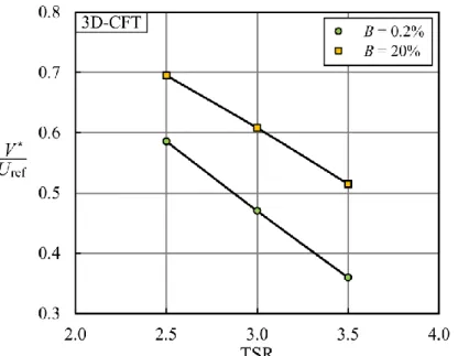
2.3.2 Effective turbine velocity ... 35
2.3.3 Effective performance curves ... 37
2.3.4 The optimal effective operating point ... 41
2.3.5 Effective force distributions at optimal effective operating point... 45
2.3.6 Implications for the EPTM development ... 55
3 The Effective Performance Turbine Model 57 3.1 Methodology ... 57
3.1.1 EPTM geometry ... 57
3.1.2 Formulation of the EPTM body force ... 59
3.1.3 Mesh and simulation setup ... 65
3.2 Results and discussion ... 66
3.2.1 Turbine performance predictions ... 66
3.2.2 Comparison of EPTM wake generation with reference CFD results ... 71
3.2.3 Flow model refinement: turbulence model modification ... 80
4 Conclusion 83
List of tables
Table 2-1. Dimensions of the reference axial-flow turbine. ... 21 Table 2-2. Dimensions of the reference cross-flow turbine. ... 23 Table 2-3. CFD domain dimensions (𝐿) and turbine spacing (𝑆) for each blockage level investigated (𝐵). ... 26 Table 2-4. Summary of the simulations for turbine performance characterization. ... 28 Table 2-5. Summary of the simulations for wake characterization. ... 29 Table 2-6. Turbine performance comparison between the URANS simulation of Kinsey and Dumas [18] used in this work with the DDES results provided by Boudreau and Dumas [16]. ... 35 Table 2-7. Performance metrics of the 2D-CFT operating at the same effective tip speed ratio in two channels of different blockage level. ... 40 Table 2-8. Characteristics of the three cases chosen for optimal effective operating point for the AFT, 2D-CFT and 3D-CFT. ... 45 Table 2-9. Characteristics of the three AFT cases chosen for the comparison of the mean force distributions. ... 51 Table 2-10. Characteristics of the three 2D-CFT cases chosen for the comparison of the mean force distributions. ... 52 Table 2-11. Characteristics of the two 3D-CFT cases chosen for the comparison of the mean force distributions. ... 53 Table 3-1. Mathematical expression of the non-dimensional volume ∀k ∗ for the each EPTM. ... 60 Table 3-2. Values of the non-dimensional frontal area 𝜆 for each EPTM. ... 64 Table 3-3. Comparison of the EPTM-AFT performance predictions in different channel blockage conditions with reference CFD results. ... 68 Table 3-4. Comparison of the EPTM-2DCFT performance predictions in different channel blockage conditions with reference CFD results. ... 68 Table 3-5. Comparison of the EPTM-3DCFT performance predictions in different channel blockage conditions with reference CFD results. ... 69
Table 3-6. Comparison of the EPTM-2DCFT performance predictions with reference CFD results at high blockage level (𝐵 = 40%) for the two identified optimal effective tip speed ratio. Interpolated results marked with a plus sign (+). ... 71
List of figures
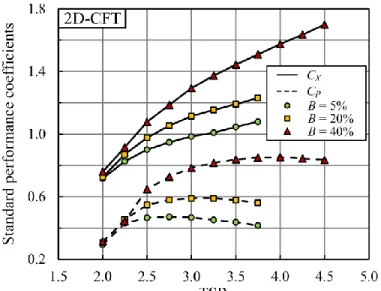
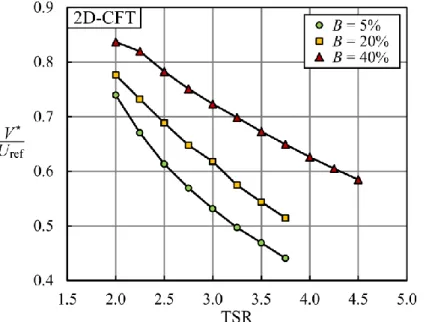
Figure 1-1. The three main types of hydrokinetic turbines: cross-flow turbine (left), axial-flow turbine (center) and oscillating-foil turbine (right). Reproduced from [2]. ... 2 Figure 1-2. Picture of the Gemini offshore wind farm located in the North Sea in the Netherlands. Reproduce from [20]. ... 4 Figure 1-3. Picture of the Horns Rev offshore wind farm illustrating the wake of upstream turbines affecting other turbines placed downstream. Reproduced from [21]. ... 6 Figure 1-4. Schematics of the cross-section of a river channel inside which turbines are deployed. ... 8 Figure 1-5. State-of-the-art full-rotor simulations of the wake structure of three typical turbine technologies. a) a one-bladed cross-flow turbine. b) an axial-flow turbine. c) an oscillating-foil turbine. Figures adapted from [15]. ... 10 Figure 1-6. Present conceptual framework of the structure of a turbine farm model. ... 11 Figure 1-7. Illustration of different actuating regions used for the modeling of AFT rotors. From left to right: full-rotor, actuator disk (AD), actuator line (AL) and actuator surface (AS). Reproduced from [22]. ... 13 Figure 2-1. Front and side views of the AFT geometry. ... 21 Figure 2-2. Geometry of the 3D-CFT (a) and the 2D-CFT (b). Turbine parts are shown in gray and the turbine centerplane is illustrated by a semi-transparent plane (3D view) and by a dotted line (2D view). ... 22 Figure 2-3. Geometry of the fluid domain of the AFT, 3D-CFT and 2D-CFT simulations. The 2D-CFT geometry is scaled up by a factor of 3 to improve visibility. ... 24 Figure 2-4. Schematics of the front view of an array formed of several AFTs (𝐵 = 40%) in a river. ... 25 Figure 2-5. Schematics of the front view of an array formed of several 3D-CFT (𝐵 = 20%) in a river. ... 25 Figure 2-6. Mesh used for the characterization of the 2D-CFT wake. a) Close-up of the mesh near the CFT. Wake mesh resolution is kept high up to 15 turbine diameters downstream. b) Close-up of the mesh near one of the CFT blades. ... 30
Figure 2-7. Domain geometry and mesh used for the characterization of the 3D-CFT wake. a) Isometric view of the domain. The turbine blades are in blue and the turbine hub is in red. b) Side view of the refined mesh region for wake capture. c) Close-up of the mesh near the CFT. d) Close-up of the mesh near one of the CFT blades. ... 31 Figure 2-8. Standard performance curves of the AFT operating at various tip speed ratios (TSR) in three channels of different blockage levels (B). ... 33 Figure 2-9. Standard performance curves of the 2D-CFT operating at various tip speed ratios (TSR) in three channels of different blockage levels (B). ... 33 Figure 2-10. Standard performance curves of the 3D-CFT operating at various tip speed ratios (TSR) in two channels of different blockage levels (B). ... 34 Figure 2-11. Effective turbine velocity ratio for the AFT operating at various tip speed ratios (TSR) in three channels of different blockage levels (B). ... 36 Figure 2-12. Effective turbine velocity ratio for the 2D-CFT operating at various tip speed ratios (TSR) in three channels of different blockage levels (B). ... 36 Figure 2-13. Effective turbine velocity ratio for the 3D-CFT operating at various tip speed ratios (TSR) in two channels of different blockage levels (B). ... 37 Figure 2-14. Effective performance curves of the AFT operating at various tip speed ratios (TSR) in three channels of different blockage levels (B). ... 38 Figure 2-15. Effective performance curves of the 2D-CFT operating at various tip speed ratios (TSR) in three channels of different blockage levels (B). ... 39 Figure 2-16. Effective performance curves of the 3D-CFT operating at various tip speed ratios (TSR) in two channels of different blockage levels (B). ... 39 Figure 2-17. Standard power coefficient function of the effective tip speed ratio for the AFT. ... 41 Figure 2-18. Standard power coefficient function of the effective tip speed ratio for the 2D-CFT. ... 42 Figure 2-19. Standard power coefficient function of the effective tip speed ratio for the 3D-CFT. Maximum power extraction zone is highlighted in red. ... 42 Figure 2-20. Normalized standard power coefficient distribution along a turbine cycle for one blade of the 2D-CFT in channels of different blockage levels. ... 44 Figure 2-21. Illustration of one of the sub-region of the volume swept by the AFT rotor. ... 46
Figure 2-22. Illustration of one of the sub-region of the volume swept by the 2D-CFT blades and of the hub sub-region. ... 47 Figure 2-23. Illustration of one of the sub-region of the volume swept by the 3D-CFT blades and of the hub sub-region. ... 47 Figure 2-24. Size of the sub-regions of the 3D-CFT swept-volume in the 𝑧-direction. ... 48 Figure 2-25. Schematics of the mean force distribution experienced by the blades of the AFT. ... 50 Figure 2-26. Axial, tangential and radial mean force distributions of the AFT operating at or near TSRopt ∗ in three different channel blockage levels 𝐵. ... 51 Figure 2-27. Schematics of the mean force distribution experienced by the 2D-CFT during a full revolution. ... 52 Figure 2-28. Streamwise and transverse mean force distributions induced by the blades of the CFT on the flow. ... 53 Figure 2-29. Evolution across a cycle of the streamwise and transverse effective force coefficients of one blade of the 3D-CFT for two blockage levels. ... 54 Figure 2-30. Spanwise distribution of the three components of the effective force coefficient for the blade of the 3D-CFT at an angular position of 𝜃 = 80° (maximum instantaneous power extraction) and two blockage levels. ... 54 Figure 3-1. Geometry of the actuating region (gray transparent region) of the EPTM-3DCFT and EPTM-2DCFT. The turbine centerplane is depicted in blue. a) isometric view. b) side view. ... 58 Figure 3-2. Geometry of the actuating region (red transparent region) of the EPTM-AFT. .... 58 Figure 3-3. Reference force distributions of the EPTM-2DCFT. ... 61 Figure 3-4. Reference force distributions 𝑐𝑋 ∗ (top), 𝑐𝑌 ∗ (middle) and 𝑐𝑍 ∗ (bottom) of the EPTM-3DCFT. ... 62 Figure 3-5. Reference force distributions 𝑐𝑋 ∗ (top), 𝑐𝑌 ∗ (middle) and 𝑐𝑍 ∗ (bottom) of the EPTM-AFT. ... 63 Figure 3-6. Mean 𝑥-velocity profiles at the turbine centerplane of the 2D-CFT and the EPTM-2DCFT (red). ... 70 Figure 3-7. Comparison of the wake recovery of the reference AFT-DDES and the EPTM-AFT (AFT-DDES simulation data provided by [16]). a) Contours of the mean streamwise velocity
fields drawn on a plane passing by the turbine axis. Only a part of the domain is displayed in the 𝑦-direction. b) Profiles of the mean streamwise velocity at different locations in the wake. ... 72 Figure 3-8. Comparison of the wake recovery of the reference 2D-CFT and the EPTM-2DCFT. a) Contours of the mean streamwise velocity fields. b) Profiles of the mean streamwise velocity at different locations in the wake. ... 73 Figure 3-9. Comparison of the wake recovery of the reference 3D-CFT and the EPTM-3DCFT. a) Contours of the mean streamwise velocity fields drawn on a plane passing by the turbine axis. Top: side view. Bottom: top view. b) Profiles of the mean streamwise velocity at different locations in the wake. Top: 𝑦-direction. Bottom: 𝑧-direction. ... 74 Figure 3-10. Comparison of the wake recovery of the three reference turbines with their associated EPTM. a) Mean wake recovery illustrated using the space-averaged mean streamwise velocity ratio. b) averaged non-dimensional mean wake recovery rate. c) Section-averaged values of the three principal mechanisms responsible for the mean wake recovery rate. ... 76 Figure 3-11. Instantaneous tangential vorticity field of the AFT-DDES. Simulation data provided by [16]. ... 79 Figure 3-12. Instantaneous z-vorticity field of the 2D-CFT. ... 79 Figure 3-13. Comparison of the wake recovery of the reference 2D-CFT with the EPTM-2DCFT and the EPTM-2DCFT with added turbulence production. a) Contours of the mean streamwise velocity ratio fields. b) Profiles of the mean streamwise velocity ratio at different locations in the wake. ... 81
List of symbols, abbreviations, subscripts and superscripts
Symbols
𝑥, 𝑦, 𝑧 cartesian coordinates 𝑟, 𝜃, 𝑧 cylindrical coordinates
𝑡 time
𝑇 time taken by the turbine to conduct a full revolution
𝐷 turbine diameter
𝑅 turbine radius
𝑑hub turbine hub diameter
𝑏 turbine span
𝑐 blade chord length
𝑁 number of blades
𝜎 turbine solidity, 𝑁𝑐/𝑅
𝐿𝑥, 𝐿𝑦, 𝐿𝑧 extent of the channel in the 𝑥, 𝑦 and 𝑧 directions
𝑆 turbine spacing
𝐴 turbine frontal area, 𝜋𝐷
2
4 (AFT), 𝑏𝐷 (CFT)
𝐴channel channel cross-sectional area, 𝐿𝑥𝐿𝑦 𝐵 channel blockage level, 𝐴/𝐴channel
𝜌 fluid density
𝜇 fluid dynamic viscosity 𝜈 fluid kinematic viscosity, 𝜇/𝜌
𝜈𝑡 eddy viscosity 𝑢𝑖 velocity 𝑈𝑖 velocity (Reynolds-averaged) 𝑝 pressure 𝑃 pressure (Reynolds-averaged) 𝑅𝑒 Reynolds number, 𝑈𝐷/𝜈
𝑄 flowrate passing through the turbine centerplane 𝑉∗ turbine effective velocity, 𝑄/𝐴
𝐹𝑥, 𝐹𝑦, 𝐹𝑧 turbine force components in the 𝑥, 𝑦 and 𝑧 directions 𝐹𝑅, 𝐹𝜃 turbine force components in the 𝑟 and 𝜃 directions 𝐶𝑋, 𝐶𝑌, 𝐶𝑍 mean force coefficients in the 𝑥, 𝑦 and 𝑧 directions,
𝐹𝑖 1 2𝜌𝑈ref2 𝐴
𝐶𝑅, 𝐶𝜃 mean force coefficients in the 𝑟 and 𝜃 directions, 𝐹𝑖 1 2𝜌𝑈ref2 𝐴
𝐶𝑅, 𝐶𝜃 mean force coefficients in the 𝑟 and 𝜃 directions, 𝐹𝑖 1 2𝜌𝑈ref2 𝐴
𝐶𝑋∗, 𝐶𝑌∗, 𝐶𝑍∗ effective force coefficients in the 𝑥, 𝑦 and 𝑧 directions, 𝐹𝑖 1 2𝜌𝑉
∗2𝐴
𝐶𝑅∗, 𝐶
𝜃∗ effective force coefficients in the 𝑟 and 𝜃 directions, 𝐹𝑖 1 2𝜌𝑉∗2𝐴
Ω turbine rotation rate in radians per second 𝑀 turbine rotor torque
𝑃 power extracted by the turbine 𝐶𝑃 mean power coefficient, 1 𝑃̅
2𝜌𝑈ref3 𝐴
𝐶𝑃∗ effective power coefficient, 1 𝑃̅ 2𝜌𝑉∗3𝐴
TSR tip-speed ratio, Ω𝑅/𝑈ref
TSR∗ effective tip-speed ratio, Ω𝑅/𝑉∗ 𝑆𝑘 turbulent kinetic energy source term
𝜁𝑘 turbulent kinetic energy production augmentation factor
Abbreviations
CFT cross-flow turbine AFT axial-flow turbine OFT oscillating-foil turbine
CFD computational fluid dynamics
AD actuator disk
AS actuator surface
BEM blade-element method
LMADT linear momentum actuator disk theory EPTM effective performance turbine model 2D-CFT two-dimensional representation of the CFT 3D-CFT three-dimensional representation of the CFT
EPTM-AFT effective performance turbine model applied to the AFT
EPTM-2DCFT effective performance turbine model applied to the 2D-CFT EPTM-3DCFT effective performance turbine model applied to the 3D-CFT RANS Reynolds-averaged Navier-Stokes
URANS unsteady Reynolds-averaged Navier-Stokes DDES delayed detached eddy simulation
SIMPLE semi-implicit method for pressure-linked equations TKEST turbulent kinetic energy source term
Subscripts and superscripts
mean or time-averaged quantities ′ fluctuating quantities
⃗⃗⃗ vectorial quantity
〈 〉 section-averaged quantities
Remerciements
Tout d’abord, j’aimerais remercier mon directeur de recherche, le professeur Guy Dumas, pour m’avoir accompagné tout au long de ma maîtrise et pour m’avoir transmis sa passion pour la mécanique des fluides. Sa rigueur, son encadrement et son dévouement ont été pour moi très précieux. Je me sens privilégié de faire partie de la grande famille qu’il a fondé au Laboratoire de Mécanique des Fluides Numérique (LMFN).
Je tiens aussi à remercier tous les collègues, stagiaires ou anciens du LMFN que j’ai eu la chance de côtoyer au cours de mes années passées au LMFN. Merci à Thomas Kinsey, Étienne Gauthier, Matthieu Boudreau, Olivier Gauvin-Tremblay, Guillaume Beardsell, Christian Perron, Philippe Côté, Jean-Christophe Veilleux, Marine Heschung et Rémi Gosselin d’avoir fait de mes premières expériences en tant que stagiaires au LMFN si agréables et d’avoir rendu le choix de continuer aux études graduées si naturel. Un merci particulier à Thomas Kinsey, pour son mentorat, son écoute et sa disponibilité. Merci aussi à Élodie Caufriez-Gingras pour l’agréable collaboration à l’été 2016, ainsi qu’à Olivier Gauvin-Tremblay avec qui j’ai eu un plaisir fou à jeter des (parfois gros) pavés dans la mare et à discuter de nos projets respectifs. Merci aussi à Thierry Villeneuve, mon fidèle partenaire de pause-café, et à Matthieu Boudreau pour toute l’entraide, les discussions enrichissantes et les matchs « déchirants » de Spike-Ball. J’aimerais également remercier ma famille et mes proches pour m’avoir soutenu durant toute la durée de mes études. Un merci particulier à Jacques Bourget, Hélène Fortier et Marcel Dallaire pour avoir continuellement cru en moi. Un gros merci aussi à mes très chers amis de One Flight
Down, Pier-Luc Bilodeau et Raphaël Lavoie. Nos jams m’auront permis maintes fois d’évacuer
le stress et votre écoute a toujours été très appréciée. Je tiens aussi à remercier Claudia Vaillancourt pour son soutien et pour toute la joie qu’elle m’apporte au quotidien.
Pour terminer, je souhaite souligner le support financier que m’ont généreusement accordé le LMFN, par le biais de la subvention CRSNG-Découverte et des projets contractuels avec MAVI Innovations et Ressources Naturelles Canada, et le Fonds de Recherche Québécois – Nature et Technologies.
Chapter 1
Introduction
1.1
Context and motivation
As the need for electrical power increases continuously across the globe and as fossil fuels become less and less accessible, exploiting renewable energy sources is now more essential than ever. Fortunately, renewable energy comes in many different forms. In Canada, renewable energy is produced from biomass, geothermal, solar, wind, oceans and hydro resources [1]. Because of its huge and diverse water resources, most of the electricity generation in Canada is produced from hydropower. In fact, Canada generated 59% of its electricity from hydroelectricity in 2015, making it the second largest producer in the world behind China [1]. Relying on hydraulic turbines, a mature and efficient technology, hydroelectricity is produced by converting the potential energy of a water reservoir into electricity. In the more recent years, another alternative renewable energy source has emerged. It is referred to as hydrokinetic power [2].
Similar to wind power, hydrokinetic power relies on the use of turbines to convert the kinetic energy of fast-flowing rivers or tidal currents into electricity. There are currently three main types of hydrokinetic turbines (Figure 1-1): cross-flow turbines (CFT; also known as vertical-axis or Darrieus-type turbines), axial-flow turbines (AFT; also known as horizontal-vertical-axis turbines) and oscillating foil turbines (OFT). Among renewable sources, hydrokinetic power has many advantages. Compared to wind and solar power, the power extracted from rivers or tidal flows is far more predictable. In addition, because water is much heavier than air, the energy density is higher in water flows than it is in winds for typical flow speeds. Hence, for the same amount of power generated, hydrokinetic turbines can be significantly smaller in scale. In
Figure 1-1. The three main types of hydrokinetic turbines: cross-flow turbine (left), axial-flow turbine (center) and oscillating-foil turbine (right). Reproduced from [2].
terms of visual pollution, hydrokinetic turbines are discreet because most of the turbine components are immerged below the surface. Moreover, deploying hydrokinetic turbines does not require the construction of dams or retaining basins, which minimizes the environmental impact. However, hydrokinetic turbines are known to operate at a smaller efficiency compared to hydraulic turbines because a larger part of the incoming flow is able to divert around the turbine.
One of the differences between river and tidal turbines resides in their size and thus in their rated power capacity. Indeed, because tidal channels are generally very large and deep compared to rivers, larger turbines can be deployed, and thus more power can be generated. As reported by Hydro-Québec, river hydrokinetic turbines rarely exceed the 400 kilowatts power output, while tidal ones can reach more than one megawatt per machine [2]. For example, the first industrial prototype of hydrokinetic turbine to be connected to the Hydro-Québec grid had a 100 kilowatts rated power output [2]. It was deployed in the St-Laurence River near Montreal in 2010. More recently, the Cape Shard Tidal consortium has successfully deployed a 2-megawatts turbine into the powerful tides of the Bay of Fundy in Nova Scotia [3].
Despite their limited power capacity, small-scale hydrokinetic turbines have the potential to be very useful regarding on-site deployment in remote communities [4]. Without access to the grid, these communities rely heavily on diesel fuel for electricity production and are thus submitted to high-energy costs. Depending on the location of the community, hydrokinetic power generation may represent a cost-effective way to produce electricity compared to diesel, while
adding diversity to the power generation systems already in place and being a source of economic development [4].
Unfortunately, because many technical, environmental and economic issues still remain unsolved, the hydrokinetic power industry has not left the experimental and pre-commercialization stages yet [1]. It is thus critical that research works continue to be carried out in order to facilitate and accelerate the growth of this emerging industry in Canada and abroad. In this spirit, numerous research works have been carried out at the LMFN. This is the research laboratory where this master’s thesis work has been conducted. Focused on both fundamental and more practical engineering research topics, the expertise at the LMFN revolves around fluid mechanics. Taking advantage of a significant supercomputing allocation granted by Compute Canada, most studies involve computational fluid dynamics (CFD) and use numerical simulations as the main investigation tool. Among the several studies carried out at the LMFN, many works have tackled the study and optimization of two distinct turbine technologies: oscillating-foil turbines ([5], [6], [7], [8], [9], [10], [11], [12]) and cross-flow turbines ([13], [14]). The wake dynamics of the three main types of hydrokinetic turbines depicted in Figure 1-1 have also been investigated at the LMFN ([15], [16]). Moreover, several works were concerned with the effects of different flow conditions on the performance of different turbine technologies. Specifically, the effects of sheared and misaligned flow have been studied [17], along with the effects of confinement ([11], [18]) and free-surface [19]. These studies at Laval University have contributed to a better understanding of both the behavior of a turbine and the impact it has on a flow.
Although hydrokinetic power is slowly growing towards maturity, more challenges related to turbine deployment in river or tidal flows have to be addressed to make it more competitive with other energy sources. At the LMFN, a new line of research addressing one of these challenges has been initiated in recent years. It is related to the optimization of turbine farm layouts. Indeed, deploying multiple turbines in dense arrays to create a farm is necessary if significant power generation is desired and to facilitate the connection to the electric grid. Such a practice is common in the context of wind power (Figure 1-2). Turbine deployment in arrays is directly applicable and desirable in the context of hydrokinetic power.
Figure 1-2. Picture of the Gemini offshore wind farm located in the North Sea in the Netherlands. Reproduce from [20].
The numerical methods necessary to conduct farm layout optimization studies have only been briefly investigated in the past at the LMFN during the master’s study of M. Oliver Gauvin-Tremblay [19] and no conclusion regarding the best method to adopt has been formulated at the time. Indeed, there is a strong desire at the LMFN to adopt a numerical methodology that would allow the study of turbine farm layouts to be carried out at a reasonable computing cost. The main motivation of the present work is thus to identify such a numerical methodology and to verify its reliability.
To introduce the reader to the subject, the following section presents the goals and challenges associated to the numerical modeling of turbine farms, along with a review of the key characteristics of modern turbine farm models. This section naturally introduces the formulation of the specific objectives of this master’s thesis.
1.2
Turbine farm modeling
1.2.1 Goals and challenges
The main goal of a turbine farm model is to predict what are the turbine performances given a specified flow condition and farm layout. Indeed, to be able to optimize the farm layout, the individual performance of each turbine needs to be available. With this information in hand, the
layout can then be improved by, for example, changing the position of the least-performing turbines.
In this work, the performance metrics of a turbine are characterized in terms of the forces it exerts on the flow,
the useful power it extracts from the flow, and
the total power losses it induces in the flow as a result of both useful power extraction and viscous dissipation.
Indeed, power extraction predictions are very important because they are directly linked to electricity production costs and thus to the project profitability. The force estimates are also of critical importance in practice for the mechanical design of the turbines and their mooring systems. The total power lost by the flow is also of interest because it is related to water level changes and might become limiting when the farm extracts a significant portion of the total available energy.
In this work, we restrict ourselves to the hydrodynamic aspects of power conversion. As a result, one should consider the useful power extraction data presented in this work as an upper limit on what can actually be expected in terms of electric power because of the unavoidable losses associated with the conversion system. Even if the characterization of these losses was integrated into the farm design process, they have no effects on the hydrodynamics at play and so they are neglected here.
While it may appear simple at first, predicting the performances of a turbine farm can be an arduous task because of the complex hydrodynamics at play. For example, when turbines are placed relatively close downstream of others, they may experience poor flow conditions induced by the wake of upstream turbines. This phenomenon, referred to as wake interference, is illustrated in the context of wind farms on Figure 1-3.
Specifically, wake flows affect the behavior of a turbine in three different ways: due to their intrinsic lower velocity, the non-uniformity of their velocity profile and their high turbulence levels. Indeed, because the power extraction of a turbine is function of the cubic power of the
Figure 1-3. Picture of the Horns Rev offshore wind farm illustrating the wake of upstream turbines affecting other turbines placed downstream. Reproduced from [21].
flow speed, a downstream turbine might extract significantly less power than a turbine operating in the first row of the farm. In fact, it is mentioned by Sanderse [22] that “Depending on the layout and the wind conditions of a wind farm, the power loss of a downstream turbine can easily reach 40% in full-wake conditions.”. In second, the non-uniformity of the wake velocity profile can alter significantly the loading distributions applied on the turbine blades [17]. This has the effect of making the turbine operate in unbalanced, off-design loading conditions. Finally, the high turbulence levels typical of turbine wakes can potentially affect the boundary layers transitions on the blades, in addition to induce strong loading fluctuations. The latter can expose the turbine to premature fatigue failures.
Surely, turbulence is not exclusive to wake flows. Most natural flows considered for turbine farm deployment exhibit a significant level of turbulence. In these turbulent flow conditions, even if the flow is uniform in the mean, the turbine performances can be affected through changes in the development of both boundary layers and wake structures. This subject has been investigated experimentally by Mycek et al. [23]. Specifically, they studied the influence of the turbulence intensity on the performances and wake recovery of a three-bladed AFT. From their results, they noted a global reduction of the turbine performances as the turbulence intensity increased. For the cases at the highest turbulence intensity, they observed relative drops of about 10% on mean drag force and power extraction. The specific value depended on the turbine
rotational speed (through the tip-speed ratio) and the inflow velocity (through the flow Reynolds number). Nevertheless, the mean drag force and power extraction were only weakly dependent (less than 2% relative) to inflow turbulence levels for the turbine operating at optimal rotating speed and at the highest Reynolds number investigated.
They also showed that the turbine wake dynamics are strongly affected by the turbulence intensity. For their high-turbulence case, they observed a much faster recovery of the wake. This beneficial aspect of upstream turbulence may allow downstream turbines to be placed much closer to upstream ones in the farm without experiencing the negative effects of wake interference. This is precisely what Mycek et al. [24] investigated in the second part of their experimental work. Specifically, they placed a second AFT of the same geometry in the wake of the first turbine operating near maximum power extraction and varied, along with the inflow turbulence intensity, the tip speed ratio of the downstream turbine and the distance between them. For a separating distance of six turbine diameters, they observed that the second turbine was able to extract about 90% of the upstream turbine power if the inflow turbulence intensity was high. Indeed, this means that the wake of the upstream turbine was nearly recovered at this distance. For their low turbulent intensity inflow, they noticed a striking difference as the downstream turbine only extracted 50% of the upstream turbine power, even if it was placed two times further downstream at twelve turbine diameters.
Similar work conducted by Blackmore, Myers and Bahaj [25] at the same facilities (belonging to the Institut Français de Recherche pour l'Exploitation de la Mer, or IFREMER) has led to the same observations. However, the experimental apparatus allowed to study the effects of the turbulent length scale together with that of the turbulent intensity. They concluded that the global effect of increasing turbulent intensity tends to reduce the turbine power extraction (about 10% relative between turbulent intensities of 6.8% and 14.3%), but that an increase of the turbulence length scale tends to improve it (about 10% relative between length scales of 0.19 and 0.51 turbine diameter).
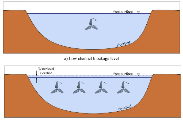
Another challenge related to the prediction of the power extracted by a turbine farm arises because the performance of a turbine can be affected by the presence of other turbines located nearby. Free-surface or riverbed proximity can also have an effect. This is especially true if the turbine farm is intended to be dense, as one would expect for river farms ([18], [26], [27]). This
phenomenon is referred to in the literature as blockage effects. Figure 1-4 illustrates two turbine deployments of different channel blockage levels.
Unlike wake interference, blockage effects are mostly beneficial to a turbine. Specifically, when channel blockage is high (as is the case in Figure 1-4b), both the magnitude of the forces exerted on the turbine and its power extraction increase compared to a low-blockage case (Figure 1-4a). This happens because a smaller part of the flow can divert the turbines in a high-blockage situation, and thus a higher flow speed is experienced by the turbine. A numerical study carried out by Kinsey and Dumas [18] has shown that a blockage level of 20% (meaning that the turbines occupy 20% of the channel cross section area) can induce a 15% increase of the turbine drag force when compared to very low blockage conditions. The associated relative increase in power extraction was found to be near 25%. These specific results were obtained for an AFT, but the authors reported similar results for a CFT as well.
In rivers or tidal channels, turbine performances may also be affected by free-surface effects. Gauvin-Tremblay [19] showed for an oscillating-foil turbine that the performance of the turbine can significantly degrade if it operates very close to the surface. A minimal depth of one blade
chord length has been considered. In addition, if multiple turbines are deployed in a river, the upstream water level may change because of the significant flow resistance (or more precisely because of the important total power lost) (Figure 1-4b). Indeed, because of mass conservation, a rise of the upstream water level leads to a decrease of the incoming flow speed and thus to a decrease of the available kinetic energy.
Another challenge related to the numerical modeling of turbine farms arises from the farm layout optimization process itself. Indeed, this optimization process has the potential to be arduous and lengthy because of the many interacting design parameters such as the number, the size and the type of turbines, along with their relative on-site positions and operating conditions. In fact, even if numerical simulations represent a great way to minimize the cost of pre-deployment studies compared to experimental tests involving expensive prototypes and facilities, every design iteration may require a large amount of time and high computational costs. Clearly, this depends on the specific numerical model employed to evaluate the farm performances for a given layout. As a matter of fact, even with supercomputing resources, it is still impractical to model more than a few complete turbine rotors in the same numerical simulation (at least as far as optimization processes are concerned). This type of high-fidelity CFD simulations, referred to here as “full-rotor simulations”, need to be conducted on several hundreds of computer processors and can take months to complete. Figure 1-5 shows some of the results of such state-of-the-art numerical simulations carried out by Boudreau and Dumas [15]. On this figure, the complex wake structure of the three turbines they investigated is illustrated with a semi-transparent representation of the vorticity field. Despite their high computational cost, these high-fidelity models can provide, through an enormous amount of high-quality data, precious insights regarding the flow behavior. In practice, however, it is evident that simpler and more cost-effective models need to be used in the context of farm layout optimization.
To be useful to farm designers however, simplified models must provide reliable results. For the different stakeholders involved in a turbine farm project, the often-large uncertainty regarding the predicted net power output represents a big risk. According to a state-of-the-sector report produced by Marine Renewables Canada in 2013 [28], this uncertainty is one of the main issues slowing the development of the marine renewable energy industry, of which the
Figure 1-5. State-of-the-art full-rotor simulations of the wake structure of three typical turbine technologies. a) a one-bladed cross-flow turbine. b) an axial-flow turbine. c) an oscillating-foil turbine. Figures adapted from [15].
hydrokinetic power industry is part. This need for reliable power output predictions has also been mentioned by Butcher in a paper reporting interviews with experts from the field [29].
1.2.2 Key characteristics of existing models
Over the years, many simplified modeling methods of varying computational cost and accuracy have been investigated. This is especially true in the field of wind energy because the latter is more mature than the hydrokinetic energy field. Notwithstanding, one should note that the methods developed for wind farms are adaptable to river or tidal farm as well. In fact, this research topic is very active in both fields and new modeling approaches are still being proposed. The following paragraphs present a review of the key characteristics of the various methods published in the literature.
According to the conceptual framework used by Sanderse [22], a farm model is constituted of two coupled sub-models: a “blade model” and a “wake model”. As their names suggest, the blade model is used to predict the performances of the turbines for a given flow condition and the wake model is used to obtain a prediction of the wakes depending on the turbine performances. However, for the sake of generality, these two model families are referred-to in this work as “turbine models” and “flow models”, respectively. This nomenclature is proposed because the terminology “blade model” suggests that only blades are considered into the model, whereas turbines also involve structures and shafts that may be incorporated. The terminology “wake model” suggests that only the wakes of the turbines are of interest, whereas the incoming flow, the bypass flow, the channel bathymetry and the free-surface behavior may all be of interest. Indeed, the turbine model and the flow model are intrinsically linked because they depend on each other. In other words, the turbine model provides inputs to the flow model and
vice-versa. Figure 1-6 illustrates the relationship between the turbine model and the flow model.
In his review of the different methods used for the modeling of wind turbines, Sanderse [22] mentioned that growing research interests had been observed at the time (in 2011) towards models that use finite-volume computational fluid dynamics (CFD) as their flow model. Despite the fact that CFD may not always be cheap in terms of computational costs, these methods are now commonly found in the literature because they offer great flexibility and accuracy. Another reason why they are chosen over other flow models such as the well-known momentum theory is that CFD flow models can take into account inherently the complex flow dynamics mentioned earlier, namely blockage effects, wake interference effects, flow turbulence and free-surface effects. The complex bathymetry of riverbeds can also be included in CFD simulations.
While the flow model is certainly very important, the most important component of a farm model remains the turbine model. To be useful to a farm designer, it is critical that the turbine model reproduces as faithfully as possible the behavior of the specific turbine selected for future deployment. In this work, the latter will be referred-to as the reference turbine.
In its simplest form, a turbine can be modelled as a constant force acting on the flow. In these circumstances, the turbine model provides the direction and the magnitude of this force, along with the way it is distributed through space. Typically, the turbine forces are applied in CFD simulations through momentum source terms which act only inside specific regions of the flow. In other words, in the form of a body force, an additional term 𝑓𝑖 is added to the Navier-Stokes
equations (written in Einstein notation):
𝜌𝜕𝑢𝑖 𝜕𝑡 + 𝜌𝑢𝑗 𝜕𝑢𝑖 𝜕𝑥𝑗 = − 𝜕𝑝 𝜕𝑥𝑖 + 𝜇 𝜕2𝑢𝑖 𝜕𝑥𝑗𝜕𝑥𝑗 + 𝑓𝑖 (1-1)
Historically, the region in which this volumetric force acts was first referred-to as an “actuator disk” (AD) because the geometry of the region (a thin cylinder) was used to replicate the geometry of AFT rotors. Now, with the development of other turbine technologies and the advancement of turbine modeling methods, the zone in which the momentum source term is applied can have different geometries depending on the specific turbine considered. For the sake of generality, these zones will be referred-to as actuating regions in this work.
Generally, in steady-state modelling, the actuating region geometry is related to the volume swept by the turbine blades. For AFTs, this approach leads to thin cylindrical geometries such as the actuator disk. However, other approaches exist such as the actuator surface (AS) and the actuator line (AL). The latter has been proposed by Sorensen [30] in 2002 and is described in greater details in the thesis of Mikkelsen [31] and Ivanell [32]. The actuator surface and actuator line approaches distinguish themselves from the actuator disk because they are intrinsically unsteady models. With the actuator line and surface methods, the actuating regions replicate the blade’s movements as they revolve around the turbine shaft instead of considering the rotor in the mean. Figure 1-7 illustrates the actuator disk, line, and surface concepts in the context of AFT rotor modeling. For visualization purposes, the actuator disk (AD) drawing is
Figure 1-7. Illustration of different actuating regions used for the modeling of AFT rotors. From left to right: full-rotor, actuator disk (AD), actuator line (AL) and actuator surface (AS). Reproduced from [22]. scaled down and only illustrates force vectors on an axisymmetrical band. Indeed, an actuator disk shares the same diameter as the reference turbine and generates forces throughout the disk. As the geometry of CFTs differ greatly from that of AFTs (Figure 1-1), annular or cylindrical actuating regions are generally preferred over that of thin disks. For example, an actuator cylinder approach has been tested by Bachant [33] and both an actuator annulus and an actuator line approach have been used by Shamsoddin and Porté-Agel [34]. The different turbine modeling methods that use actuating regions are categorized by Sanderse [22] as “generalized actuator methods”.
Compared to full-rotor turbine models, actuator models are mostly advantageous because they avoid the use of very large meshes associated to the resolution of the thin boundary layers developing on the rotor. They also avoid the sometimes-challenging meshing process of complex rotor geometries. Thus, they are economical in terms of human time and computational costs. Moreover, many actuator models are designed to be used within the framework of steady-state simulations, reducing even more the computational costs compared to unsteady simulations.
To determine the forces generated by the actuating regions, one may use several approaches. The classical, yet very popular, blade-element method (BEM) is one of them. In brief, the BEM consists of dividing the turbine rotor into multiple sections (the blade-elements) of which the aerodynamic characteristics are assumed known. For example, force coefficients such as lift and drag coefficients may be given as a function of the angle of attack. Conceptually, this results in an analogous division of the actuating regions. On Figure 1-7, each illustrated force vector on the AL would correspond to a specific element. For the AD, the division into blade-elements leads rather to several axisymmetric bands. By estimating the relative flow speed at
each of the blade-elements and the associated angle of attack, the forces generated by each blade-element can be obtained. To calculate the global turbine loading, one has to sum the contributions of each blade-element.
Indeed, the BEM has the potential to generate representative force distributions through the actuating region (be it an actuator disk, line, or surface). However, as mentioned by Sørensen [21], the main drawback of this method is that it is very sensitive to the blade-section force coefficients used. Typically, two-dimensional steady-state blade-section coefficients are used. Thus, obtaining reliable force distributions from blade-element calculations can be a challenge in some cases, especially when unsteady turbine technologies such as the cross-flow turbine are involved. In addition, many sub-models are needed to take into account the actual physics at play on a real blade such as flow unsteadiness, tip-loss effects and dynamic stall [21]. For the interested reader, Hansen et al. [35] published a review of the various sub-models proposed in the literature. To avoid the use of sub-models and their inherent uncertainties, some authors have used the results of full-rotor simulations to obtain the right force coefficients for each blade-element ([36], [37], [38], [39]). Indeed, much effort has been dedicated to improving BEMs to reproduce as faithfully as possible the actual loading experienced by the turbine. Another important weakness of blade-element methods is related to the accurate determination of the angle of attack of each blade-element. Even if it appears simple conceptually, it is known to be challenging in practice because it depends strongly on where the blade-element velocity triangle is computed and because the velocity gradients are usually very large near the actuating regions [39]. Indeed, because aerodynamic force coefficients are strong functions of the angle of attack, a small error in the angle of attack calculation can lead to large force calculation errors. There exist other methods than blade-element ones to prescribe the forces of the actuating region. For example, van der Laan et al. [40] proposed to use the force distribution of a known rotor (the National Renewable Energy Laboratory 5-MW reference wind turbine [41]) and to scale this force distribution with global turbine force coefficients such as the turbine drag coefficient 𝐶𝑥. The latter is typically expressed as
𝐹𝑥 = 𝐶𝑥∙
1 2𝜌𝑈ref
where 𝜌 is the fluid density, 𝑈ref is a reference velocity scale usually taken as the inflow velocity and 𝐴 is the turbine frontal area. Other turbine force components are defined analogously. However, the formulation of Equation (1-2) is not ideal because, for a given turbine size and inflow velocity 𝑈ref, a turbine can experience different local flow conditions depending on channel blockage and wake interference ([40], [42]). Thus, the turbine may induce more or less forces on the flow and this would change the value of the drag force coefficient. For this reason, authors such as Meyers and Meneveau [42] have argued that the inflow velocity may not be the best suited to scale the forces generated by the actuating region in the context of farm modeling. Indeed, to account for the change in flow speed induced by wake interference or blockage effects, one should use a more local velocity scale to adjust the forces generated by the actuating region. Without using exactly the same definitions, many authors have been using a local velocity scale in their turbine models ([40], [42], [43], [44], [45], [46], [47] and [38]). Of all the proposed definitions, that of Meyers and Meneveau [42] is particularly appealing because of its simplicity and conceptual meaning. Their definition relates the local flow velocity experienced by a turbine to the flowrate 𝑄 passing through it. While they refer to this local velocity scale as the “axial disk-averaged velocity”, it is referred-to in this work as the effective turbine velocity 𝑉∗. Thus, according to this definition, we have
𝑉∗ ≡𝑄
𝐴 (1-3)
Readers familiar with the Linear Momentum Actuator Disk Theory (LMADT) can relate directly this definition of 𝑉∗ with the concept of axial induction factor 𝑎 [48]. This relation is provided in Equation (1-4).
𝑉∗ = (1 − 𝑎)𝑈
ref (1-4)
Since a local velocity scale is used, appropriate force and power coefficients need to be defined for coherence. These coefficients differ from the standard force and power coefficients that are defined with the inflow velocity 𝑈ref (as in Equation (1-2)). In the LMADT literature, the coefficients based on 𝑉∗ are usually referred to as “disk” or “local” force coefficients ([48], [49], [50]). Van der Laan et al. [40] simply described these coefficients as “alternative force coefficients”. In this work, they are referred-to as effective force coefficients to remind of their
link with the effective velocity 𝑉∗. To distinguish them from the standard force coefficients such
as the turbine drag coefficient 𝐶𝑥, they are marked with a star superscript (*). Hence, when using
effective force coefficients, the coherent formulation of the turbine drag force is
𝐹𝑥 = 𝐶𝑥∗∙
1 2𝜌𝑉
∗2𝐴 (1-5)
Although this formulation brings advantages to the turbine model (such as the adaptability to local flow speeds), obtaining the values of the effective force coefficients of a turbine is not that straightforward because it involves the calculation of the effective turbine velocity 𝑉∗. For example, in their work, Meyers and Meneveau [42] obtained representative values of effective force coefficients by making several hypotheses and making blade-element momentum theory calculations. Their model used uniform force distributions across the actuator disk.
In the work of Shives and Crawford [46], the values of the effective performance coefficients of the turbine are obtained by a series of calibration simulations. In these simulations, the known turbine force is applied inside the actuating regions of the turbine model and a local velocity scale is obtained from the flow field. This velocity scale, which is defined as the mean streamwise velocity inside the actuating region, is then used to compute the effective force coefficients using equation (1-5). Finally, the forces are distributed through the actuating region using the force distribution of Mycek et al. [23]. The works of Shives and Crawford followed the works of van der Laan et al. [40], whom have been using the force distributions of Jonkman et al. [41].
To the knowledge of the author, the effective performance coefficients of a turbine have never been characterized using only results derived from experimental measurements or high-fidelity full-rotor simulations. The latter idea is part of the original approach adopted and presented in this thesis.
The reference force distribution methods are advantageous compared to blade-element methods because they avoid most of their issues such as the calculation of the blade-elements’ angles of attack. One can also argue that they are more robust because they use a single velocity scale value (usually space and time-averaged such as 𝑉∗), as opposed to multiple velocity scales local
distributions through experimental tests or full-rotor CFD simulations, tip-loss effects and dynamic stall are naturally accounted for. Thus, these methods seem more appropriate for unsteady turbine technologies such as the CFT. Moreover, the reference force distribution methods can also be used to extract not only the force distributions on the turbine blades, but also on other parts such as blade arms, shrouds or shafts, making them more general and flexible.
1.3
Specific objectives and scope of work
Let us first recall that the main motivation of the present research work is to identify a numerical methodology that would allow the study of turbine farm layouts to be carried out at a reasonable computing cost and to verify its reliability.
As presented in section 1.2.1, to be the most useful, a farm model should behave correctly with regards to channel blockage effects, wake interference, turbulence and free-surface effects. In addition, it should be the most cost-effective as possible while maintaining an adequate reliability. Moreover, the modeling methodology should be systematically applicable to any specific hydrokinetic turbine technology.
Based on the study of the available literature provided in section 1.2.2, one observes that modern farm models possess the following key characteristics:
they use CFD to predict the behavior of the flow in which the turbines are immerged; the turbines are represented using actuating regions in which a body force (or momentum
source term) is added to the Navier-Stokes equations;
the actuating regions have a geometry representative of that of the reference turbine; the magnitude of the forces generated by the actuating region is determined using a local
velocity scale and appropriate force coefficients; and
the forces are distributed through the actuating region using either blade-element methods or reference force distribution methods to reproduce as faithfully as possible the actual mean force distribution of the reference turbine.
In the present thesis, it has been chosen to investigate an original modeling approach that shares all these key characteristics. Hence, a modeling approach has been developed and is proposed
in this work. It is referred-to as the Effective Performance Turbine Model, or EPTM. This name has been chosen because the forces of the actuating region are scaled with the effective turbine velocity 𝑉∗ and the associated effective force coefficients. In the proposed EPTM approach, the
effective force coefficients of the turbine are obtained solely using results of a high-fidelity, full-rotor CFD simulation. This is in contrast to other approaches described in section 1.2.2. The forces are distributed through the actuating region using reference force distributions also obtained from the full-rotor CFD simulation. Thus, the EPTM does not follow a blade-element approach (with all its shortcomings). In addition, to limit the computational costs related to the EPTM, attention is devoted only to the reproduction of the mean turbine performances, rather than on its precise instantaneous performances. In this manner, the EPTM calculations use a steady-state CFD flow resolution.
In order to gather the appropriate inputs needed to develop an EPTM and to create a solid database for the EPTM assessment, the second chapter of this master’s thesis is devoted to a full-rotor CFD investigation of three reference turbines. Specifically, an axial-flow turbine (AFT), a 2D cross-flow turbine (2D-CFT) and a 3D extension of the latter (3D-CFT) are studied. As both cross-flow and axial-flow turbines are considered, it will be possible to assess the ability of the EPTM approach to model different types of turbine.
As a first development step, this study only covers the characterization of the performances of the turbines with regards to channel blockage effects because it is considered as the main actor of farm flow dynamics if wake interactions are avoided. Thus, the effects on the turbines performances of other farm flow dynamics such as wake interference, strong inflow turbulence and free-surface effects are not considered in this work. Indeed, the production of another reference database would be necessary to assess the performance of the EPTM approach with regards to these effects.
In the third chapter of this master’s thesis, the EPTM approach is described in greater details and is used to model the three reference turbines. The three resulting models are referred-to as the EPTM-AFT, the EPTM-2DCFT and the EPTM-3DCFT. For different channel blockage levels, the predictions of the turbine performances provided by each of the EPTM are compared to the reference CFD database presented in chapter 2. In addition, as it is of importance that the
wake of the EPTM matches that of its reference turbine in the context of potential wake interference, a wake comparison is conducted. Finally, a brief discussion regarding a possible modification to the turbulence modeling approach used is presented and applied in EPTM-2DCFT simulations to improve the far-wake predictions.
Chapter 2
Full-rotor reference simulations
In this chapter, a full-rotor CFD investigation of the three reference turbines considered in this work is presented. The aim of this investigation is to gather the appropriate inputs needed to develop an EPTM for each turbine and to create a solid database for the assessment of the latter. To begin, the geometry and principal characteristics of the reference turbines are described. Then, the numerical methodology used is detailed. Results regarding the standard performance curves of the turbines, the effective velocity scale they experience and their effective performance curves are presented. In addition, the force distributions at maximum power extraction are obtained. At last, the implication of those results for the development of a turbine model are discussed.
2.1
Turbines geometry
The geometry of the reference turbines is illustrated in Figure 2-1 and Figure 2-2. The plane section defining the turbine centerplane is also drawn on these figures, along with the typical orientation of the incoming flow 𝑈ref. Specific information on the turbines geometries is also provided in Table 2-1 and Table 2-2.
The AFT rotor geometry was provided by the research group of professor Curran Crawford at University of Victoria in Canada. More information regarding that rotor geometry can be found in a technical report by Klaptocz et al. [51] or in the master’ thesis of Perron [17].This turbine has been chosen because it is representative of typical axial-flow turbines and had been investigated in previous CFD works conducted at the LMFN ([16], [18], [17]).
The cross-flow turbine geometry was provided by Mavi Innovations Inc. as part of the project “Quantifying Extractable Power from a Stretch of River Using an Array of MHK Turbines” [26]. A simplified version of the complete turbine is considered here as no connection between the turbine shaft and the blades has been included in the simulations.
Table 2-1. Dimensions of the reference axial-flow turbine.
Parameter Value
Chord-to-diameter ratio, 𝑐/𝐷 from 0.252 (root) to 0.087 (tip) Blade-length to diameter ratio, 𝑏/𝐷 0.4 (from root to tip)
Frontal area, 𝐴 𝜋𝐷2/4
Number of Blades, N 3
Blade Profile SD8020
(with geometrical twist) Hub-to-turbine diameter ratio, 𝑑hub/𝐷 0.087
Figure 2-2. Geometry of the 3D-CFT (a) and the 2D-CFT (b). Turbine parts are shown in gray and the turbine centerplane is illustrated by a semi-transparent plane (3D view) and by a dotted line (2D view).
Table 2-2. Dimensions of the reference cross-flow turbine.
Parameter Cross-flow Turbine
Diameter-to-chord ratio, 𝐷/𝑐 14
Blade aspect ratio, 𝑏/𝑐 10.5
Turbine aspect ratio, 𝑏/𝐷 0.75
Frontal area, 𝐴 𝑏 ∙ 𝐷
Number of Blades, N 3
Blade Profile NACA 63-021
Hub-to-turbine diameter ratio, 𝑑hub/𝐷 0.053
Solidity, 𝜎 = 𝑁𝑐/𝑅 0.428
2.2
Methodology
The numerical simulations of the AFT presented in this work originate from a CFD database produced as part of a previous project conducted at the LMFN [18]. However, as some of the performance metrics of interest in this work had not been monitored at the time, the simulations have been re-run for a few turbine revolutions. This CFD work has been carried out with the help of Élodie Caufriez-Gingras [52] as part of her internship at the LMFN.
The numerical simulations of the 2D-CFT and the 3D-CFT have been carried out as part of the project “Quantifying Extractable Power from a Stretch of River Using an Array of MHK Turbines” [26] in which the author of this master thesis has participated. This collaborative research project, sponsored by Natural Resource Canada, involved Mavi Innovations Inc. (as the principal investigator), the National Research Council – Ocean, Coastal and Engineering, Lambda2 – Engineering Simulations and the LMFN. The numerical methodology used in the present thesis is analogous to that presented and validated in details in a paper by Kinsey and Dumas [18].
2.2.1 Simulation setup
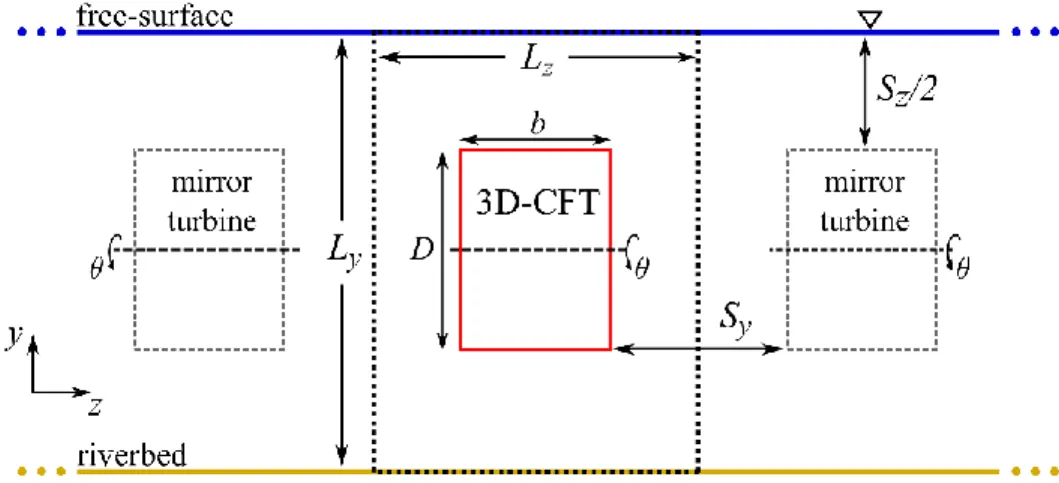
To investigate the effects of blockage on the performance of the turbines, the latter are centered in closed slip-wall channels of different sizes and having the same aspect ratio as the turbine (Figure 2-3).
Figure 2-3. Geometry of the fluid domain of the AFT, 3D-CFT and 2D-CFT simulations. The 2D-CFT geometry is scaled up by a factor of 3 to improve visibility.
Figure 2-4. Schematics of the front view of an array formed of several AFTs (𝐵 = 40%) in a river. The resulting channel blockage level 𝐵 is given by
𝐵 = 𝐴/𝐴channel (2-1)
where 𝐴channel is the cross-sectional area of the fluid domain. For the 2D-CFT simulations, the blockage level is rather expressed as
𝐵 = 𝐷/𝐿 (2-2)
where 𝐿 is the vertical extent of the fluid domain (see Figure 2-3 (c) ).
As depicted in Figure 2-4 and Figure 2-5 for the AFT and 3D-CFT respectively, this modeling approach mimics a single-row array deployment of several equally-spaced turbines facing a river flow where all boundaries (including free-surface and riverbed) are accounted for as symmetry planes. The domain cross-section dimensions (𝐿/𝐷) are provided in Table 2-3, along
Table 2-3. CFD domain dimensions (𝐿) and turbine spacing (𝑆) for each blockage level investigated (𝐵).
Turbine Parameter Values
𝐵 0.2% 10% 19.6% AFT 𝐿/𝐷 40 5.6 4.0 𝑆/𝐷 39 4.6 3.0 𝐵 5% 20% 40% 2D-CFT 𝐿/𝐷 20 5.0 2.5 𝑆/𝐷 19 4.0 1.5 𝐵 0.17% - 20% 𝐿𝑦/𝐷 22.4 - 2.24 3D-CFT 𝐿𝑧/𝐷 16.75 - 1.68 𝑆𝑦/𝐷 21.4 - 1.24 𝑆𝑧/𝐷 16.0 - 0.93
with the resulting turbine spacing (𝑆/𝐷) for each blockage levels investigated.
For both turbine technologies in this work, an incompressible Unsteady Reynolds-Averaged Navier-Stokes (URANS) approach has been used to resolve the flow around the full geometry of the turbine rotor. All simulations have been performed using the StarCCM+ commercial software. The URANS approach is used in many engineering applications because it avoids the
very expensive resolution of the smallest-scales of turbulence. Instead, a model is used to predict
the effects of turbulence on the flow. The turbulence model used is the well-known two-equation 𝑘 − 𝜔 SST model of Menter [53], which blends a 𝑘 − 𝜔 model that acts very close to the walls (down to the viscous sub-layer), to a 𝑘 − 𝜖 model that acts in the far-field. For the CFT simulations, the curvature-correction option has been enabled. This option limits the production of turbulent kinetic energy inside regions of the flow where strong streamline curvature is present. This option has not been enabled in the AFT simulations of Kinsey and Dumas [18], and so it is not included in the present work either. In addition, the Durbin Scale Limiter option has been enabled in all simulations. This option prevents the non-physical growth of turbulent kinetic energy near stagnation points by imposing a lower limit on the turbulence time scale. For the AFT, a order coupled flow algorithm is used and for the two CFTs, a second-order SIMPLE (Semi-Implicit Method for Pressure-Linked Equations) segregated flow algorithm is used.