»¬ ¼·½·°´·²» ±« °7½·¿´·¬7 Ö«®§æ
´»
벶·» ÉßÒÙ
³»®½®»¼· ïî ±½¬±¾®» îðïêÏ«¿²¬·¬¿¬·ª» ¿²¿´§· ±º ½¸®±³¿¬·² ¼§²¿³·½ ¿²¼ ²«½´»¿® ¹»±³»¬®§ ·² ´·ª·²¹
§»¿¬ ½»´´
ÛÜ ÞÍÞ æ Þ·±´±¹·» ¬®«½¬«®¿´» »¬ º±²½¬·±²²»´´» Ô¿¾±®¿¬±·®» ¼» Þ·±´±¹·» Ó±´7½«´¿·®» Û«½¿®§±¬» øÔÞÓÛ÷ ó ËÓÎ ëðçç ÝÒÎÍ Õ»®¬·² ÞÇÍÌÎ×ÝÕÇ Ð®±º»»«® ¼» ˲·ª»®·¬7ô ̱«´±«» ô Ú®¿²½» Ю7·¼»²¬ Ù·´´» ÝØßÎÊ×Ò Ý¸¿®¹7 ¼» ®»½¸»®½¸»ô ×ÙÞÓÝô ×´´µ·®½¸ ο°°±®¬»«® ׿¾»´´» ÍßÙÑÌ Ü·®»½¬»«® ¼» ®»½¸»®½¸»ô ×ÞÙÝô Þ±®¼»¿«¨ ο°°±®¬»«® ͧ´ª·» ÌÑËÎÒ×ÛÎ Ü·®»½¬»«® ¼» ®»½¸»®½¸»ô ÔÞÝÓÝÐô ̱«´±«» Û¨¿³·²¿¬»«® Õ¿®·²» ÜËÞÎßÒß Ü·®»½¬»«® ¼» ®»½¸»®½¸»ô ÝÛßô Ú±²¬»²¿§ Û¨¿³·²¿¬»«® Ö«´·»² ÓÑÆÆ×ÝÑÒßÝÝ× Ó¿2¬®» ¼» ½±²º7®»²½» ôÔÐÌÓÝô п®· Û¨¿³·²¿¬»«® Ñ´·ª·»® ÙßÜßÔ Ü·®»½¬»«® ¼» ®»½¸»®½¸»ô ÔÞÓÛô ̱«´±«» ݱ󼷮»½¬»«® ¼» ¬¸8» ß«®7´·»² ÞßÒÝßËÜ Ý¸¿®¹7 ¼» ®»½¸»®½¸»ô ÔßßÍô ̱«´±«» ݱ󼷮»½¬»«® ¼» ¬¸8» Ñ´·ª·»® ÙßÜßÔ ¿²¼ ß«®7´·»² ÞßÒÝßËÜFirst and foremost, I would like to give my sincere respects to my supervisors Olivier Gadal and Aurélien Bancaud. It is exactly them who brought me here three years ago, and helped me initiate my PhD projects. They allow me to knock their office door at any time when I encountered problems in biology and mathematics, and every time they could offer me an appropriate solution. I highly appreciate their guidance, discussion, patience, and encouragement during my PhD study. I also thank them for providing me opportunities to go for the international conferences.
I am appreciative of the help from Christophe Normand. I feel very lucky to be in the same group as him. Christophe is such a skilled person who trained me much about the biology technologies. In addition he is also an easy-going person who helped me much of my life in France, such as accommodations and entertainment.
Isabelle Léger, I am deeply indebted to her. She has a broad knowledge of biology. I benefited much from the discussion with her. Every time when I was confused by problems (either cell biology or biophysics), she always proposed me to make cross-checks on imperceptible points. She also taught me much about the culture in France. I also need thank her help in the modification of my PhD thesis. Without her help, I cannot easily arrive at the end for sure.
I particularly thank Alain Kamgoue, who taught me how to use Matlab. He is such a talented mathematician. Each time he can help me to find a best way to resolve the problem I met in mathematic (especially in Matlab and R language field). I cannot forget his intelligent forever.
I thank Sylvain Cantaloube, who trained me much how to use the confocal microscope. In addition, he also helped me much in the analysis of the microscope images.
Many thanks to my collegues Christophe Dez, Frédéric Beckouët, Marta Kwapisz, Lise Dauban and Tommy Darrière. They are so kind to me and always help me much in my life. I feel so pleasure to be in the same group with them. Frédéric Beckouët taught me many things in molecular biology; Marta Kwapisz helped me to prepare the mutant strains I need in my project; Lise Dauban and Tommy Darrière also helped me many in the basic biology experiments. You guys made me a confortable environment for learning and discussing. I will memorize great time spent with you all for life.
I must thank the members of my thesis committee: Sylvie Tournier and Julien Mozziconacci. Each year I would present my work of the previous year to them, and each time they gave me many interesting suggestions from their own field.
arrange all the travel tickets and the restaurant for my international conference. Without her, I cannot participate these international conferences so easy and happy.
I am grateful to the jury members of my PhD defense. I thank Isabelle Sagot and Gilles Charvin for their acceptance being my referees, and reading my manuscript carefully. The remarks from them are also appreciated. I also must thank Karine Dubrana as the examiner of my defense, the talk about chromatin dynamics with her also helped me understand my project much more.
I thank Prof. Kerstin Bystricky as the president to host my PhD defense. I also thank her and Silvia Kocanova’s care during the “Advanced workshop on interdisciplinary views on chromosome structure and function” in Italy.
Also, all friends are appreciated for their hospitality and kindness.
I cannot forget all activities (travelling, party, chatting……) with my friends, Faqiang Leng, Weikai Zong, Diandian Ke, Zhouye Chen, Yu Chen, Congzhang Gao. I like to play games with these guys and I enjoy our party time. I will remember these days all my life.
Finally, I would like to thank my father Fujian Wang, my mother Erqin Wang and my brother Junjie Wang for their continuous supports and their family love. My parents as farmers have been working very hard to afford all costs of my education sinc the first day I stepped into the school. I now reward them with a doctorate son. My girfriend, Tingting Bi, she is always standing by my side and giving me endless love. It is much difficult to keep a long-distance relation spanning six to seven time zones. We have together passed through the hard time. Without her supports, I would not be the person who I am today. Thank you, my darling.
A special thanks to China Scholarship Council (CSC) as the main financial support during 09/2013-09/2016.
王仁杰
1
SUMMARY
Chromosome high-order architecture has been increasingly studied over the last decade thanks to technological breakthroughs in imaging and in molecular biology. It is now established that structural organization of the genome is a key determinant in all aspects of genomic transactions. Although several models have been proposed to describe the folding of chromosomes, the physical principles governing their organization are still largely debated. Nucleus is the cell’s compartment in which chromosomal DNA is confined. Geometrical constrains imposed by nuclear confinement are expected to affect high-order chromatin structure. However, the quantitative measurement of the influence of the nuclear structure on the genome organization is unknown, mostly because accurate nuclear shape and size determination is technically challenging.
This thesis was organized along two axes: the first aim of my project was to study the dynamics and physical properties of chromatin in the S. cerevisiae yeast nucleus. The second objective I had was to develop techniques to detect and analyze the nuclear 3D geomtry with high accuracy.
Ribosomal DNA (rDNA) is the repetitive sequences which clustered in the nucleolus in budding yeast cells. First, I studied the dynamics of non-rDNA and rDNA in exponentially growing yeast cells. The motion of the non-rDNA could be modeled as a two-regime Rouse model. The dynamics of rDNA was very different and could be fitted well with a power law of scaling exponent ~0.7. Furthermore, we compared the dynamics change of non-rDNA in WT strains and temperature sensitive (TS) strains before and after global transcription was actived. The fluctuations of non-rDNA genes after transcriptional inactivation were much higher than in the control strain. The motion of the chromatin was still consistent with the Rouse model. We propose that the chromatin in living cells is best modeled using an alternative Rouse model: the “branched Rouse polymer”.
Second, we developed “NucQuant”, an automated fluorescent localization method which accurately interpolates the nuclear envelope (NE) position in a large cell population. This algorithm includes a post-acquisition correction of the measurement bias due to spherical aberration along Z-axis. “NucQuant” can be used to determine the nuclear geometry under different conditions. Combined with microfluidic technology, I could accurately estimate the shape and size of the nuclei in 3D along entire cell cycle. “NucQuant” was also utilized to detect the distribution of nuclear pore complexes (NPCs) clusters under different conditions, and revealed their non-homogeneous distribution. Upon reduction of the nucleolar volume,
2
NPCs are concentrated in the NE flanking the nucleolus, suggesting a physical link between NPCs and the nucleolar content.
In conclusion, we have further explored the biophysical properties of the chromatin, and proposed that chromatin in the nucleoplasm can be modeled as "branched Rouse polymers". Moreover, we have developed “NucQuant”, a set of computational tools to facilitate the study of the nuclear shape and size. Further analysis will be required to reveal the links between the nucleus geometry and the chromatin dynamics.
3
RESUME
L'analyse de l'organisation à grande échelle des chromosomes, par des approches d'imagerie et de biologie moléculaire, constitue un enjeu important de la biologie. Il est maintenant établi que l'organisation structurelle du génome est un facteur déterminant dans tous les aspects des « transactions » génomiques: transcription, recombinaison, réplication et réparation de l'ADN. Bien que plusieurs modèles aient été proposés pour décrire l’arrangement spatial des chromosomes, les principes physiques qui sous-tendent l'organisation et la dynamique de la chromatine dans le noyau sont encore largement débattus. Le noyau est le compartiment de la cellule dans lequel l'ADN chromosomique est confiné. Cependant, la mesure quantitative de l'influence de la structure nucléaire sur l'organisation du génome est délicate, principalement du fait d'un manque d'outils pour déterminer précisément la taille et la forme du noyau.
Cette thèse est organisée en deux parties: le premier axe de mon projet était d'étudier la dynamique et les propriétés physiques de la chromatine dans le noyau de la levure S.
cerevisiae. Le deuxième axe visait à développer des techniques pour détecter et quantifier la
forme et la taille du noyau avec une grande précision.
Dans les cellules de levure en croissance exponentielle, j'ai étudié la dynamique et les propriétés physiques de la chromatine de deux régions génomiques distinctes: les régions codant les ARN ribosomiques regroupés au sein d’un domaine nucléaire, le nucléole, et la chromatine du nucléoplasme. Le mouvement de la chromatine nucléoplasmique peut être modélisé par une dynamique dite de « Rouse ». La dynamique de la chromatine nucléolaire est très différente et son déplacement caractérisé par une loi de puissance d'exposant ~ 0,7. En outre, nous avons comparé le changement de la dynamique de la chromatine nucléoplasmique dans une souche sauvage et une souche porteuse d'un allèle sensible à la température (ts) permettant une inactivation conditionnelle de la transcription par l'ARN polymérase II. Les mouvements chromatiniens sont beaucoup plus importants après inactivation transcriptionnelle que dans la souche témoin. Cependant, les mouvements de la chromatine restent caractérisés par une dynamique dite de « Rouse ». Nous proposons donc un modèle biophysique prenant en compte ces résultats : le modèle de polymère dit "branched-Rouse". Dans la deuxième partie, j'ai développé "NucQuant", une méthode d'analyse d'image permettant la localisation automatique de la position de l'enveloppe nucléaire du noyau de levures. Cet algorithme comprend une correction post-acquisition de l'erreur de mesure due à l'aberration sphérique le long de l'axe Z. "NucQuant" peut être utilisée pour déterminer la géométrie nucléaire dans de grandes populations cellulaires. En combinant « NucQuant » à la
4
technologie microfluidique, nous avons pu estimer avec précision la forme et la taille des noyaux en trois dimensions (3D) au cours du cycle cellulaire. "NucQuant" a également été utilisé pour détecter la distribution des regroupements locaux de complexes de pore nucléaire (NPCs) dans des conditions différentes, et a révélé leur répartition non homogène le long de l’enveloppe nucléaire. En particulier, nous avons pu montrer une distribution particulière sur la région de l’enveloppe en contact avec le nucléole.
En conclusion, nous avons étudié les propriétés biophysiques de la chromatine, et proposé un modèle dit "branched Rouse-polymer" pour rendre compte de ces propriétés. De plus, nous avons développé "NucQuant", un algorithme d'analyse d'image permettant de faciliter l'étude de la forme et la taille nucléaire. Ces deux travaux combinés vont permettre l’étude des liens entre la géométrie du noyau et la dynamique de la chromatine.
5 Table of Contents SUMMARY ... 1 RESUME ... 3 TABLE OF CONTENTS ... 5 FIGURE LIST ... 8 ABBREVIATIONS ... 9 INTRODUCTION ... 11
1. The chromosome organization in space ... 12
1.1 Chromatin structure ... 12
1.1.1 The DNA molecule ... 12
1.1.2 Nucleosomes ... 14
1.1.3 10 nm chromatin fibers ... 14
1.1.4 The controversial “30 nm” chromatin fiber ... 17
1.2 The chromosome spatial organization ... 19
1.2.1 Condensed mitotic chromosomes ... 19
1.2.2 Euchromatin and heterochromatin ... 21
1.2.3 Chromosome territory ... 22
1.2.4 Chromosome conformation ... 24
1.2.5 Computational model of yeast chromosome ... 32
1.2.6 Gene position and gene territory ... 35
1.2.7 Chromatin dynamics ... 40
1.3 Summary ... 46
2. Nuclear shape and size ... 47
2.1 The nuclear organization ... 47
2.1.1 The spindle pole body ... 47
2.1.2 Telomeres are distributed at the nuclear periphery ... 49
6
2.1.4 Nuclear pore complexes ... 53
2.2 Plasticity of nuclear envelope and nuclear size ... 55
2.3 The techniques used to analyze the nuclear shape and size ... 59
2.3.1 EM and EM-based techniques ... 59
2.3.2 Tomography techniques ... 62
2.3.3 Fluorescent microscopy ... 64
2.4 Summary ... 67
3. Overview ... 68
RESULTS ... 69
1. The dynamics of the chromatin in nucleoplasm and nucleolus ... 70
1.1 Objective and summary ... 70
1.2 Review: “Principles of chromatin organization in yeast: relevance of polymer models to describe nuclear organization and dynamics" ... 71
1.3 Extended discussion-the dynamics of the rDNA ... 79
2. The influence of transcription on chromatin dynamics ... 81
2.1 Objective and summary ... 81
2.2 Draft of manuscript: "Analysis of chromatin fluctuations in yeast reveals the transcription-dependent properties of chromosomes" ... 81
3. Determination of the nuclear geometry in living yeast cells... 99
3.1 Objective and summary ... 99
3.2 Submitted manuscript: "High resolution microscopy reveals the nuclear shape of budding yeast during cell cycle and in various biological states" ... 100
3.3 Extended discussion ... 144
3.3.1 Heterogeneity of the nuclear shape in cell population ... 144
3.3.2 The organization of the nucleolus ... 146
CONCLUSION AND PERSPECTIVES ... 148
1. The dynamics of non-rDNA and rDNA chromatin ... 149
7
3. Determination of the nuclear shape and size ... 152
REFERENCE ... 155
APPENDIX ... 174
1. Utilization of “NucQuant” ... 175
1.1 Installation ... 175
1.2 How to use “NucQuant” ... 175
1.2.1 Input the figures and crop the cells ... 176
1.2.2 Extract the NPC position, nuclear center, nucleolus segmentation and the nucleolar centroid ... 177
1.2.3 Class the data ... 178
1.2.4 Quality control ... 178
1.2.5 Correc the aberration along Z axis ... 178
1.2.6 Align the nuclei ... 179
1.2.7 Calculate the NPC distribution ... 179
2. Published: "Decoding the principles underlying the frequency of association with nucleoli for RNA Polymerase III-transcribed genes in budding yeast" ... 180
3. Published: ''High-throughput live-cell microscopy analysis of association between chromosome domains and the nucleolus in S.cerevisiae'' ………...195
8
Figure list
Figure 1. DNA structure an gene expressionFigure 2. The nucleolosme and chromosome structures
Figure 3. The two main models of the “30 nm” chromatin fibers Figure 4. The organization of condensed mitotic chromosomes
Figure 5. The chromosome territories and the chromosome territory-interchromatin compartment model Figure 6. The outline of the chromosome conformation capture (3C) and 3C-based techniques
Figure 7. The “fractal globule” model of the human chromosomes Figure 8. Schematic representation of the yeast nucleus
Figure 9. The chromosomes conformation in the S. cerevisiae Figure 10. The stratistical constrained random encounter model
Figure 11. Conputational model of the dynamic interphase yeast nucleus Figure 12. Nucloc to study the gene position
Figure 13. The gene territories of 15 loci along chromosome XII
Figure 14. Positions of loci along the chromosome XII relative to the nuclear and nucleolar centers determined experimentally and predicted by computational modeling
Figure 15. Tracking the gene motion in living cells Figure 16. The MSD of three different diffusion models Figure 17. The Rouse polymer model
Figure 18. The chromatin dynamics and confinements vary along the length of the chromosome. Figure 19. The structure and organization of the spindle pole body (SPB)
Figure 20. The nucleolar organization
Figure 21. Overall structure of Nuclear Pore Complex (NPC) Figure 22. Nuclear shape is dynamic
Figure 23. Nuclear morphology of yeast L1489 prepared by cryo-fixation and chemical fixation techniques, respectively
Figure 24. 3D reconstruction of the S. cerevisiae nuclear envelope analyzed by TEM Figure 25. 3D reconstruction of the yeast cells by SBF-SEM technology
Figure 26. Reconstruction of the yeast cells by X-ray tomography
Figure 27. Reconstruct the nuclear envelope by fluorescent microscopy in 2D Figure 28. The dynamics of rDNA
Figure 29. The heterogeneity of the nuclear shape
Figure 30. The change of the nucleolus structure after the cells enter quiescence Figure 31. The “ideal” Rouse model and the chromosome models in living yeast cells. Figure 32. The detection of the nuclear shape based on structured-illumination microscopy
9
ABBREVIATIONS
DNA Deoxyribonucleic acid
RNA ribonucleic acid
mRNA messenger RNA
A adenine
T thymine
C cytosine
G guanine
U uracil
NMR nuclear magnetic resonance
bp base pair
Å Ångstrom
TEM transmission electron microscopy
NRL nucleosome repeat lengths
CEMOVIS cryo-EM of vitreous sections SAXS small-angle X-ray scattering
CTs chromosome territories
FISH fluorescent in situ hybridization
IC interchromatin compartment
CT-IC chromosome territory-interchromatin compartment
3C chromosome conformation capture
4C 3C-on chip or circular 3C
5C 3C carbon copy
rDNA ribosomal DNA
NE nuclear envelope
SPB spindle pole body
CEN centromeres
TEL telomeres
NPC nuclear pore complex
tRNA transfer RNA
FROS fluorescent repressor-operator system
10
SNR signal to noise ratio
DH-PSF Double-Helix Point Spread Function
fBm fractional Brownian motion
MTs microtubules
MTOC microtubule-organizing center
EM electron microscopy
INM inner nuclear membrane
SUN Sad1p and UNC-84
KASH Klarsicht, ANC-1 and Syne homology LINC Linker of Nucleoskeleton and Cytoskeleton
FCs fibrillar centers
DFC dense fibrillar component
GC granular component
IGS intergenic spacers
RENT regulator of nucleolar silencing and telophase exit
RFB replication fork barrier
Nups nucleoporins
DIC differential interference contrast
SBF-SEM serial block-face scanning electron microscopy
ET electron tomography
HVEM high-voltage electron microscope
STEM scanning transmission electron microscopy
PSF point spread function
μm micrometer
nm nanometer
TS temperature sensitive
PVP poly-vinylpyrrolidone
11
Chapter I
Introduction
12
1. The chromosome organization in space
Chromosome spatial organization plays a key role in transcriptional regulation, DNA repair and replication. How do chromosomes organize in the eukaryotic nucleus is still an open question. In the following chapter of the introduction, I will present a general overview of the chromatin structure, chromosome spatial organization in the eukaryotic nucleus and the techniques used to study the chromosome structure and organization.
1.1 Chromatin structure 1.1.1 The DNA molecule
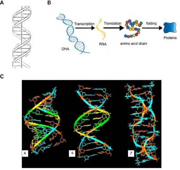
Deoxyribonucleic acid (DNA) is the molecule which carries the genetic instructions used for the formation of all compounds within the cells, such as proteins and Ribonucleic acid (RNA). Most genomic DNA consists of two biopolymer strands, coiled around a common axis; these two strands are composed of nucleotides. The genetic information is stored in the nucleotides sequence. Each nucleotide is composed of a deoxyribose, a phosphate group and a kind of nitrogenous base, either adenine (A), thymine (T), cytosine (C) or guanine (G). The nucleotides are linked together by a specific hydrogen-bond, to form a double helix (Watson and Crick, 1953b) (Figure 1A). Genetic information is expressed in two steps: first the genomic information coded in DNA is transmitted to a messenger known as messenger RNA (mRNA). RNA is a polymer of ribonucleotides in which thiamine (T) is replaced by a different nucleotide, uracil (U). The information in mRNA is then translated by an RNA based ribozyme, the ribosome, into a sequence of amino acids that forms a protein (Figure 1B). Results from X-ray diffraction, nuclear magnetic resonance (NMR) or other spectroscopic studies have shown that the DNA molecule adapts its structure according to the environment. This leads to polymorphism of the DNA structure. The three billion base pairs in the human genome exhibit a variety of structural polymorphisms which is important for the biological packaging as well as functions of DNA. B-DNA is the most commonly found structure in vivo by far. However, DNA repeat-sequences can also form several non-B DNA structures such as the G-quadruplex, the i-motif and Z-DNA (Choi and Majima, 2011; Doluca et al., 2013). Various DNA structures have been characterized as A, B, C, etc. (Bansal, 2003; Ghosh and Bansal, 2003). The currently accepted three major DNA configurations include the A-DNA, the DNA and the Z-DNA (Ghosh and Bansal, 2003) (Figure 1C). A-DNA and B-DNA are all right-handed double helix. A-B-DNA was observed under conditions of low
13
hydration; it has 11 nucleotides per turn and the projected displacement along the overall helical axis can be as low as 2.4 Å. B-DNA is the closest to the original Watson-Crick model with a near-perfect 10 units per turn and the projected displacement is ~3.4 Å; it was observed under the conditions of relative high hydration (Ghosh and Bansal, 2003; Lu et al., 2000). Unlike the A- and B-DNA, Z-DNA is a left-handed duplex structure with 12 nucleotides per turn and helix pitch is ~3 Å (Bernal et al., 2015).
Figure 1. DNA structure and gene expression
A. The double helix structure of the DNA proposed by Watson and Crick in 1953. From (Watson and Crick, 1953b).
B. Schema of the gene expression process.
C. Three possible helix structures: from left to right, the structures of A, B and Z DNA. From (Bansal, 2003).
14
X-ray diffraction, NMR or other spectroscopic techniques are used to characterize DNA conformation in vitro but, in vivo configuration of DNA molecule is still challenging. The human nucleus of 10 µm in diameter contains ~2 m of linear DNA (Watson and Crick, 1953). Nucleus in budding yeast is often described as a sphere of radius ~1 µm (Berger et al., 2008). Electron microscopic analysis indicates that the yeast nuclear DNA can be isolated as linear molecules ranging in size from 50 µm (1.2 × 10⁸ daltons) to 355 µm (8.4 × 10⁸ daltons) (Petes et al., 1973). To duplicate and segregate the genomic DNA, the long DNA sequence is organized in a condensed structure made of DNA and proteins to fit into the cell nucleus: the chromatin in eukaryotic cells.
1.1.2 Nucleosomes
The nucleosome is the fundamental unit of chromatin. It is formed by a pool of 8 polypeptides (histones) around which 145 DNA base pairs (bp) are wrapped in 1.65 turns (Absolom and Van Regenmortel, 1977; Fischle et al., 2003; Thomas and Furber, 1976). The histone octamer is composed of eight proteins, two of each core histones H2A, H2B, H3 and H4 (Hansen, 2002). The histone octamer is assembled with one H3/H4 tetramer and two H2A/H2B dimers (Figure 2A). Each histone has both an N-terminal tail and a C-terminal histone-fold. X-ray crystallography of the structural details of the nucleosome core indicates that the histone N-terminal tails can extend from one nucleosome and contact with adjacent nucleosomes (Davey et al., 2002; Luger et al., 1997). Modifications of these tails affect the inter-nucleosomal interactions and allow recruitment of specific protein complexes therefore affecting the overall chromatin structure (Dorigo et al., 2003; Shogren-Knaak et al., 2006). The modification of the histone tails is regulating accessibility of chromatin to transcription and many other DNA processes, are defined as the "histone code" (Strahl and Allis, 2000). 1.1.3 10 nm chromatin fibers
The so-called 10 nm fiber corresponds to nucleosome core particles more or less regularly spaced on the genome that form a string of beads, with short stretches of bare DNA- the linker DNA- connecting adjacent nucleosomes (Figure 2B).
Since the linker DNA should be phased with respect to the histones core, the precise orientation of a nucleosome relative to the previous one is largely determined by the linker DNA length and by the torsional constraint of the fiber (Barbi et al., 2012). The short size of the linker DNA is hardly compatible with its bending, so one can assume the linkers as
15
straight. This assumption helps researchers to describe the chromatin structure by the entry-exit angle α, the rotational angle β and the linker length (Woodcock et al., 1993) (Figure 2C). A change in α and β modifies the fiber architecture and consequently induces a rotation of one strand end with respect to the other. However, in vivo, the linker DNA length is variable depending on organisms, tissues and genomic regions and is usually associated with the H1 class of linker histone. The alternative nucleosomes spacing has significant influence on the chromatin fiber plasticity (Recouvreux et al., 2011).
In addition, the linker DNA crossing state has also significant impact on the chromatin fiber structure. According to their position at the exit of a nucleosome, the linker DNA can adopt three main states. The negatively crossed state corresponds to the standard crystallographic structure; in the positively crossed state, the two linkers DNA cross instead in the opposite, positive way; and in the open state, the DNA is partially unwrapped from the nucleosome core histones and linkers DNA do not cross anymore (De Lucia et al., 1999; Sivolob et al., 2003) (Figure 2D).
All these variations can result in the formation of irregular fibers in vivo.
The physical properties of the chromatin fibers may govern the structural changes necessary for the functioning and dynamics of chromatin. So it is important to understand the higher-order organization of the chromatin.
16
Figure 2. The nucleosome and chromosome structures.
A. Schematic representation of the assembly of the core histones wrapped by the DNA to form one nucleosome. Each histone octamer contains one H3/H4 tetramer and two H2A/H2B dimers. From Wikipedia, author Richard Wheeler (Zephyris).
B. The nucleosome arrays form the “10 nm” chromatin fiber. The “10 nm” fibers compact to form the “30 nm” chromatin fibers which was for long time considered to represent a higher order chromatin organization in vivo. From (Maeshima et al., 2010).
C. Schematic of the DNA winding pattern along two neighbouring nucleosomes. From (Recouvreux et al., 2011).
17
D. The states of the Linker DNA. From (Recouvreux et al., 2011).
1.1.4 The controversial “30 nm” chromatin fiber
The nucleosome has long been assumed to compact into irregular fibers with ~30 nm diameter (Bednar et al., 1998; Robinson et al., 2006). Although “30 nm” fibers have been observed in vitro (Finch and Klug, 1976), their existence in vivo remains an open and highly debated question since most attempts to visualize these fibers in vivo have failed so far (Joti et al., 2012; Maeshima et al., 2010).
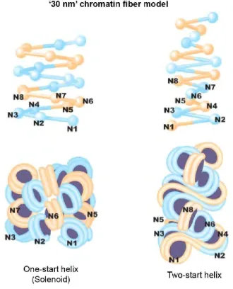
Two main “30 nm” structures have been described: one-start helix with interdigitated nucleosomes, called ‘solenoid’ model, and ‘two-start helix’ model (Robinson and Rhodes, 2006). Solenoid fibers in which consecutive nucleosomes are located close to one another in the fiber and compacting into a simple one-start helix have been observed by conventional transmission electron microscopy (TEM) (Thomas and Furber, 1976). The ‘two-start helix’ model has been extrapolated from the crystal structure of a four-nucleosomes core array lacking the linker histone. In this model, the nucleosomes are arranged in a zigzag manner: a nucleosome in the fiber is bound to the second neighbor but not to the closest (Schalch et al., 2005) (Figure 3). Grigoryev’s team found that under certain conditions in vitro these two models can be simultaneously present in a 30 nm chromatin fiber (Grigoryev et al., 2009).
In vivo, the length of the linkers DNA is not identical which will result in many various
folding. Routh’s group found that the nucleosome repeat length (NRL) and the linker histone can influence the chromatin higher-order structure. Only the 197-bp NRL array with the linker histone H1 variant, H5, can form 30 nm fibers. The 167-bp NRL array displays a thinner fiber (~20 nm) (Routh et al., 2008). Rhodes's lab found two different fiber structures which were determined by the linker DNA length: when the linker DNA length is 10-40 bp the produced fibers have a diameter of 33 nm, and the fibers have a diameter of 44 nm when the linker DNA length is from 50 to 70 bp (Robinson et al., 2006).
We should note that, all these studies were all led in vitro or on purified fibers. Any small variations in experimental conditions will impact the regulation of the nucleosomes arrays. In
vivo, the length of the linkers DNA is varied, the flexibility of each nucleosome also. If the
“30 nm” chromatin fiber exists in vivo is still controversial. More recently, cryo-EM of vitreous sections (CEMOVIS) or small-angle X-ray scattering (SAXS) techniques were used
18
to study the nucleosomes organization of HeLa cells: the results showed that no matter in interphase or in mitotic chromatins, there was no “30 nm” chromatin structure formation. In
vivo, nucleosomes concentration is high. Therefore, nucleosome fibers are forced to
interdigitate with others, which can interfere with the formation and maintenance of the static 30-nm chromatin fiber and lead to the “polymer melt” behaviour (Joti et al., 2012; Maeshima et al., 2010).
Figure 3. The two main models of the “30 nm” chromatin fibers. The one-start helix is an interdigitated solenoid. The first nucleosome (N1) in the fiber contacts with its fifth (N5) and sixth (N6) neighbors. In the two-start model, nucleosomes are arranged in a zigzag manner. The first nucleosome (N1) in the fiber binds to the second-neighbor nucleosome (N3). Blue and orange represent the alternate nucleosome pairs. From (Maeshima et al., 2010).
19
1.2 The chromosome spatial organization
The linear array of nucleosomes that comprises the primary structure of chromatin is folded and condensed to different degrees in nuclei and chromosomes forming “higher order structures”. The chromosomes in mitosis are highly condensed and moved independently by the mitotic spindle apparatus. After cell division, the compacted chromatin is decondensed in interphase phases (Antonin and Neumann, 2016). In this part, I will introduce the spatial organization of the chromosomes in mitosis and interphase.
1.2.1 Condensed mitotic chromosomes
Mitosis is a part of the cell cycle in which chromosomes are separated into two identical sets. The mitotic chromosome structure in metazoan cells has been observed by light microscopy (Rieder and Palazzo, 1992). To avoid the truncation of chromosome arms during cell division and to facilitate proper separation and segregation of sister chromatids, the mitotic chromosomes are highly condensed with an iconic structure of X-shaped (Figure 4A). How mitotic chromosomes organize is still controversial. Solid evidence suggests that the topoisomerase II and condensin complexes contribute to this condensation (Hudson et al., 2009; Lau and Csankovszki, 2014; Maeshima and Laemmli, 2003; Moser and Swedlow, 2011). There are two main models to explain the mitotic chromosome organization: hierarchical folding model and radial loop model (Antonin and Neumann, 2016) (Figure 4B). Crick and co-workers proposed hierarchical folding model, which proposes that the mitosis chromosomes are formed by a hierarchical helical folding of ‘30 nm’ chromatin fibers (Bak et al., 1977). The radial loop model suggests that the mitotic chromosomes are folded with radial loop model, in which mitotic chromatin forms series of chromatin loops which are attached to a central chromosome scaffold axis (Maeshima and Eltsov, 2008). Immunofluorescence of the isolated human chromosome topoisomerase IIα and the condensin I component indicates that the chromosome scaffold components have axial distributions at the center of each chromatid in the mitotic chromosome (Maeshima and Laemmli, 2003). Recent Hi-C data also proved the mitotic chromosome organized with radial loop model (See section 1.2.4). However, if the ’30 nm’ chromatin fibers exist in the living cells is still controversial.
20
Figure 4. The organization of condensed mitotic chromosomes.
A. The structure of a mitotic chromosome: two sister chromatids are anchored each other through centromere. Adapted from (Antonin and Neumann, 2016).
B. Two main models of the mitotic chromatin organization. Adapted from (Antonin and Neumann, 2016).
C. In mitotic chromosomes, the nucleosome fibers exist in a highly disordered, interdigitated state like a ‘polymer melt’ that undergoes dynamic movement. Adapted from (Maeshima et al., 2010).
To study the chromosome organization in living cells, the highest resolution microscopic technics is achieved using cryo-EM of vitreous sections (CEMOVIS), but with the cost of low
21
contrast. Cells are collected and frozen by high-pressure freezing, then they are sectioned and the ultrathin sections are observed directly under a cryo-EM with no chemical fixation or staining which guarantees the cellular structures in a close-to-native state (Maeshima et al., 2010). Maeshima et al. observed the human mitotic chromosomes by using this technique and they did not find any higher-order structures including “30 nm” chromatin fibers formation; their results suggest that the nucleosomes fiber exists in a highly disordered 10 nm fiber, in an interdigitated state like a ‘polymer melt’ that undergoes dynamic movement (Maeshima et al., 2010) (Figure 4C). Since the thickness of the cryo-EM section is only ~70 nm, this prevents the observation of a whole chromosome organization. Joti and colleagues utilized small-angle X-ray scattering (SAXS), which can detect periodic structures in noncrystalline materials in solutions, to observe the chromatin structures of HeLa cells in mitosis and interphase. They found that, no matter in interphase or mitosis, there was no ‘30 nm’ chromatin structure formation in cells (Joti et al., 2012). Nishino et al. also found that, in human mitotic HeLa chromatin, there was no regular structure >11 nm detected (Nishino et al., 2012).
Actually, the “10 nm” fiber is high dynamic because the nucleosomes are dynamic (~50 nm/30 ms). So, we think that the chromatin consists of dynamic and disordered “10 nm” fibers. The chromosome can be seen as one polymer chain and the dynamic folding can offer a driving force for chromosome condensation and segregation (Maeshima et al., 2014; Nozaki et al., 2013).
In mitosis, the chromosomes are highly compacted to facilitate the segregation of their chromatids. After cell division, the compacted chromatin is decondensed to re-establish its interphase states (Antonin and Neumann, 2016). Interphase is the phase in which cells spend most of its life, the DNA replication, transcription and most of the genome transactions take place during interphase. In next sections, I will focus on the interphase chromosome organization in space.
1.2.2 Euchromatin and heterochromatin
Electron microscopy has shown that in metazoan nucleus, there are at least two structurally distinct chromatins in the nucleus in interphase, one is euchromatin and the other is heterchromatin (Albert et al., 2012; Tooze and Davies, 1967). Euchromatin is more dynamic and uncondensed. Euchromatin is often associated with transcriptionally active regions (Adkins et al., 2004). Unlike euchromatin, heterochromatin is condensed around functional
22
chromosome structures such as centromeres and telomeres, it is genes poor and can silence the expression of the genes embedded in it (Grewal and Moazed, 2003). Heterochromatin is largely transcriptionally inert. However, it plays key roles in chromosome inheritance, genome stability, dosage compensation (X-inactivation) in mammals (Lam et al., 2005). Solid evidence show that heterochromatin is required for the cohesion of the sister chromatids at centromeres and proper chromosome segregation (Bernard et al., 2001; Hall et al., 2003). Grewal’s team also found that the formation of the heterochromatin structures at telomeres can maintain their stability (Hall et al., 2003). As for localization close to the nuclear envelope, nucleoli are often surrounded by a shell of heterochromatin which is realted to the establishment and maintenance of silencing of non-rDNA-related genomec regions (McStay and Grummt, 2008).
The chromatin state are not static (Grewal and Jia, 2007). There are many factors that can influence the chromatin structure, including chromatin associated proteins, histones, linker DNA and DNA methylation. Although many studies over the past few decades have established the basic properties of the heterochromatin and euchromatin, it is still not clear how chromatin participate the cellular processes.
1.2.3 Chromosome territory
Although the “10 nm” chromatin fibers are highly dynamic (see 1.2.1), the chromosomes are not randomly organized in the nucleus. The chromosomes “prefer” to occupy specific regions in the nucleus named “chromosome territories” (CTs). The concept of CTs was first suggested for animal cell nuclei by Carl Rabl in 1885 and the name was first introduced by Theodor Boveri in 1909 (Cremer and Cremer, 2010). The fluorescent in situ hybridization (FISH) techniques enabled the generation of chromosome specific painting probes used for the direct visualization of chromosomes in many species (Bolzer et al., 2005; Manuelidis, 1985; Schardin et al., 1985) (Figure 5A). Bolzer et al. utilized FISH to mape simultaneously all chromosomes in human interphase nuclei. The map showed that the small chromosomes were organized closer to the nuclear center and the larger chromosomes located closer to the nuclear periphery (Bolzer et al., 2005). Cremer’s group combining FISH techniques and 3D-microscopy, could reconstruct the spatial arrangement of targeted DNA sequences in the nucleus. The new generation confocal microscopes allowed the distinct observation of at least five different targets at the same time (Cremer et al., 2008).
23
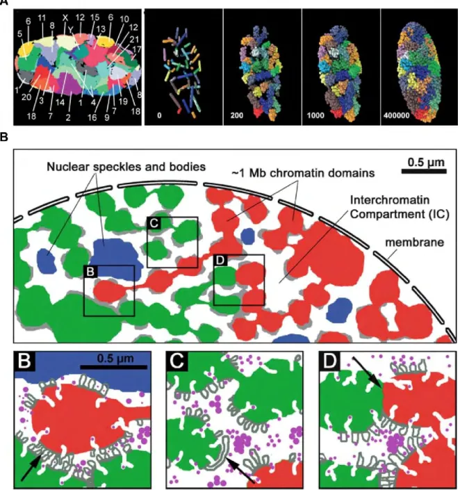
Figure 5. The chromosome territories and the chromosome territory-interchromatin compartment model.
A. 24-Color 3D FISH technologies allowed the visualization of the 46 human chromosomes in the nucleus. From (Bolzer et al., 2005).
B. Illustration of a partial interphase nucleus with differentially colored higher-ordered CTs (red and green) from neighboring CTs separated by the interchromatin compartment (IC) (white). Blue regions represent integrated IC channel network with nuclear speckles and bodies which expand between CTs. Gray regions represent perichromatin regions which locate at the periphery of the CTs. Narrow IC channels allow for the direct contact of loops from neighboring CTs (arrow, B). For the broad IC channel, the larger loop (arrow, C) expands along the perichromatin region. The arrow in D represents the direct contact between neighboring CTs. From (Albiez et al., 2006).
24
3D-FISH technique used to analyze the chromosome organization in different cell types, these studies indicated that the nuclear geometrical constrains influence CTs; CTs distribution also correlated with the genes density on the chromosome (Neusser et al., 2007). However, FISH cannot reveal the internal structure of the CTs and their interactions with neighboring CTs. Peter Lichter and colleagues defined the interchromatin compartment (IC) as the network-like space expanding mainly around CTs with little penetration into the CT interior (Zirbel et al., 1993). The chromosome territory-interchromatin compartment (CT-IC) model assumes that IC expands between chromatin domains both in the interior and the periphery of CT (Albiez et al., 2006) (Figure 5B).
These methods and models clearly show the arrangement of the CTs in the nucleus. However, we should note that FISH cannot be used for living cells, since cells must be fixed before hybridization with the probe (Rodriguez and Bjerling, 2013). In addition, limited by resolution, microscopy lacks the ability to highlight the sub-organization of the chromosomes inside the CTs. This limitation is addressed by the emergence of very different experimental approaches based on chromosome conformation capture (3C).
1.2.4 Chromosome conformation
1.2.4.1 The technical breakthrough of chromosome conformation capture: 3C-technologies
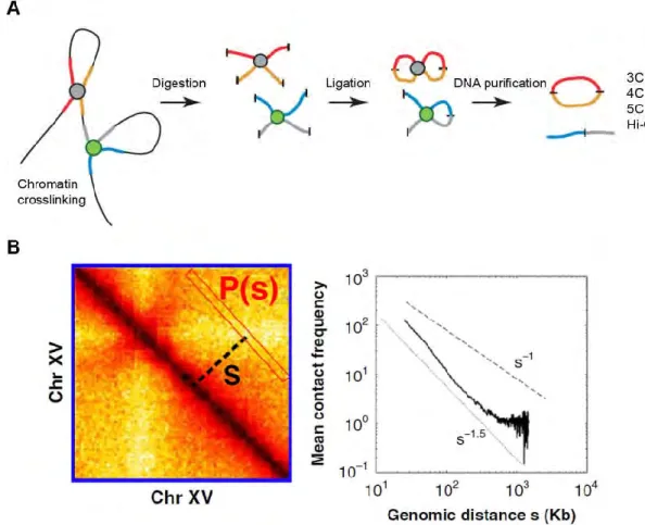
Over the last decade, the newly developed technique of chromosome conformation capture (3C) mapping the interactions between chromosomes, has significantly improved the observational resolution on the chromosomes organization (Dekker et al., 2002). For classical 3C techniques, cells are first treated with formaldehyde to covalently link the chromatin segments that are in close spatial proximity. Then, crosslinked chromatin is digested by a restriction enzyme and the restriction fragments are ligated together to form unique hybrid DNA molecules. Finally, the DNA is purified by standard phenol/chloroform extraction and analyzed (Dekker et al., 2002) (Figure 6A). The 3C products represent the chromatin fragments that may be separated by large genomic distances or located on different chromosomes, but are close in 3D. Classical 3C techniques measure the contact frequency of the genomic loci in close proximity within the nucleus (Dekker et al., 2013; Montavon and Duboule, 2012). Most 3C analysis typically cover only ten to several hundreds Kb (Naumova et al., 2012). Several techniques have been developed based on 3C to increase the throughput.
25
3C-on-Chip or circular 3C (4C) techniques allows the detection of the genome-wide interactions of one selected locus after selective amplification of this region by inverse PCR performed on the 3C products (Simonis et al., 2006; van Steensel and Dekker, 2010). 3C carbon copy (5C) techniques can identify all interactions among multiple selected loci. The specific mixture of 5C oligonucleotides is used to anneal and ligate the 3C library; this step is used to generate the 5C library. Then the 5C library is amplified by PCR for analysis (Dostie et al., 2006). Hi-C techniques, collectively named 3C-technologies provide a view of chromatin interactions map through whole genome (Belton et al., 2012; Lieberman-Aiden et al., 2009).
Figure 6. The outline of the chromosome conformation capture (3C) and 3C-based techniques.
A. Overview of 3C and 3C-derived techniques strategy. Crosslinked chromatin is digested with a restriction enzyme and the restriction fragments are ligated together to form unique hybrid DNA molecules. Finally the ligated DNA is purified and analyzed. From (Montavon and Duboule, 2012).
B. The analysis of the ligated DNA content produces the contact density map (left) and based on this, it is easy to correlate contact frequecy and the genomic distance (right). From (Wang et al., 2015).
26
3C and 3C-derived techniques allow to detect and quantify physical contacts between DNA segments (Figure 6B), yielding massive quantitative data about genome architecture at the level of large cell populations.
1.2.4.2 Chromosome conformation according chromosome conformation capture methods
These techniques can be applied to the spatial organization of entire genomes in organisms from bacteria to human (Lieberman-Aiden et al., 2009; Umbarger et al., 2011). In 2009, Lieberman-Aiden and colleagues used Hi-C to construct the contact maps of the human genome in interphase. The contact maps immediately showed some interesting features. Firstly, the contact probability between loci on one chromosome was always larger than the contact probability between loci on different chromosomes: this result confirms the existence of chromosome territories. Also, the small genes-rich chromosomes localized preferentially in the nuclear center by FISH studies, were found to interact preferentially with each other. Based on the contact frequencies, the authors suggested a ‘fractal globule’ model, a knot-free conformation that enables maximally dense packing while preserving the ability to easily fold and unfold any genomic region. This highly compact state would be formed by an unentangled polymer that would crumple into a series of small globules in a ‘beads-on-a-string’ configuration (Lieberman-Aiden et al., 2009) (Figure 7).
Further, study of the human cells chromosomes also show that long-range interactions are highly nonrandom and the same DNA fragments often interacting together (Botta et al., 2010). The longer range interactions drive the formation of compact globules along chromosomes (Sanyal et al., 2011). 5C and Hi-C maps also indicate that the mitotic chromosomes adopt a linearly-organized longitudinally compressed array of consecutive chromatin loops, these loops are irregular and would form a uniform density “melt” which is consistent with the EM and SAXS studies (Joti et al., 2012; Maeshima et al., 2010; Naumova et al., 2013).
27
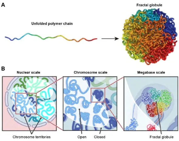
Figure 7. The “fractal globule” model of the human chromosomes. Adapted from (Lieberman-Aiden et al., 2009).
A. A fractal globule. The polymer chains are unknotted. Genomically close loci tend to remain close in 3D, leading to monochromatic blocks both on the surface and in cross-section (not shown).
B. The genome architecture of the “fractal globule” model at three scales. At nuclear scale, chromosomes (blue, cyan, green) occupy distinct territories (chromosome territories). At chromosome scale, individual chromosomes weave back-and-forth between the open and closed chromatin compartments. At the megabase scale, the chromosome consists of a series of fractal globules.
In general, the size of the genomic DNA, and the frequency of repeated DNA sequences, will impact the density of the contacts. Due to unambiguous assembly, repeated DNA sequences are excluded from the 3C analysis or should be studied independently (Cournac et al., 2016). For a similar amount of “reads”, the larger the genomic DNA, the lower resolution of the contact map (Lieberman-Aiden et al., 2009). Therefore, highest resolution using 3C-technologies is achieved with small genomes and limited repeated DNA, such as the bacteria
C. Caulobacter or the budding yeast S. Cerevisiae (Dekker et al., 2002; Umbarger et al.,
28
specific interactions with higher resolution than data collected on the complex, repeated diploid genome of metazoan cells.
1.2.4.3 Yeast genome to explore chromosome conformation
The budding yeast Saccharomyces cerevisiae is an unicellular organism that can be grown in very well controlled chemical and physical conditions. S. cerevisiae is the first eukaryote with its entire genome sequenced (Goffeau et al., 1996). Within eucaryotic phylum, yeast belongs to the same supergroup than metazoan, the opisthokonts (Wainright et al., 1993). This classification is based on the existence of a common ancestor of fungi and animals. Note that the denomination "higher eukaryots", including two distantly related groups, multicellular plantae and metazoan, opposed to "lower eukaryots" as yeast, will not be used here. Each S.
cerevisiae nucleus contains 16 relatively small chromosomes, comprising between 230 and
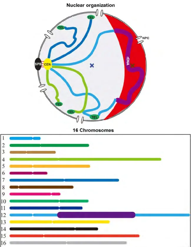
1500 kb DNA, plus ~100-200 copies of ribosomal genes (rDNA) encompassing 1-2 Mb on the chromosome XII (Figure 8). The budding yeast has played a major role in understanding the eukaryotic chromosome organization in interphase (Taddei and Gasser, 2012). Despite its small size, budding yeast has become a unique model that recaptitulates some of the main features of metazoan chromosome, and ultimately help to understand the human biology (Ostergaard et al., 2000).
In all eukaryots, chromosomes are separated from the cytoplasm by the nuclear envelope (NE). In budding yeast, NE remains closed during the entire life cycle, including mitosis. Past researches have uncovered few structural features characterizing the budding yeast nucleus in interphase: the spindle pole body (SPB), centromeres (CEN), telomeres (TEL), and the nucleolus. In interphase, the nucleolus is organized in a crescent-shaped structure adjacent to the nuclear envelope (NE) and contains quasi-exclusively genes coding ribosomal RNA (rDNA) present on the right arm of the chromosome XII. Diametrically opposed to the nucleolus, the SPB tethers the CEN during the entire cell cycle via microtubules to centromere-bound kinetochore complex (Bystricky et al., 2005a; Duan et al., 2010; Yang et al., 1989; Zimmer and Fabre, 2011). TEL are localized in clusters at the NE (Gotta et al., 1996; Klein et al., 1992). These contraints result in chromosome arms extending from CEN toward the nucleolus and periphery, defining a Rabl-like conformation (Figure 8).
29
Figure 8. Schematic representation of the yeast nucleus. Chromosome arms are depicted in color lines and their centromeres (CEN) (yellow circle) are anchored to spindle pole body (SPB) (black circle) by microtubules (red lines). All of the telomeres (TEL) (green circle) are distributed near the nuclear envelope (NE) (double-black-line circle). The nucleolus (red crescent part) is organized around the rDNA (bold purple line). Nuclear pore complexes (NPCs) are embedded in the envelope to control the nucleo-cytoplasmic transport of molecules.
30
High resolution 5C contact map of budding yeast genome was obtained in 2010 by the Noble lab (Duan et al., 2010). A computational challenge raised by 3C-technology is to reconstruct spatial distances from observed contacts between genomic loci. To achieve this goal, it is required to plot the average measured contact frequencies as function of genomic distances (Figure 6B). Then the genomic distances were transformed into spatial distances by assuming a DNA compaction in chromatin of 130 bp/nm (based on 110-150 bp/nm range estimated previously) and implicitly assuming a straight fiber geometry (Bystricky et al., 2004; Duan et al., 2010). Duan et al. identified the intra- and inter-chromosomal interactions in yeast nucleus by combining 4C and largely parallel sequencing. The genome-wide contact frequencies were then used to reconstruct a 3D model of all 16 chromosomes in the nucleus (Figure 9A). This model reproduces the features of yeast chromosome organization (Rabl-like). In addition, this model is compatible with preferential clustering of tranfer RNA (tRNA) coding genes in the nucleus (Duan et al., 2010).
Julien Mozziconacci and co-workers also created one computationally effective algorithm to reconstruct the yeast genome organization in 3D based on the Hi-C data (the genome-wide contact map) (Lesne et al., 2014). Based on this algorithm, we could reconstruct the 3D structure of chromosomes in yeast which recapitulates known features of yeast genome organization such as strong CEN clustering, weaker TEL colocalization and the spatial segregation of long and short chromosomal arms (Figure 9B). In addition, the finding that contact frequency P(s) follows a power law decrease with genomic distance s characterized by an exponent close to -1 (P(s) ~ s-1.08) is in agreement with the crumple globule model (Wang et al., 2015).
The advances of the C-technologies can help to reconstruct the chromosome organization based on the contact frequency between chromosome segments. However, because the contact frequency is an averaged frequency of a large cell population, a single structural model is not sufficient to reflect all the spatial features of the genome. It is increasingly clear that computational model of chromatin polymer is an indispendable complement for a better understanding of chromosome organization.
31
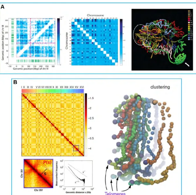
Figure 9. The chromosomes conformation in the S. cerevisiae.
A. Based on 5C techniques to detect the intra- (left, Chromosome III) and inter-chromosomal (middle) interactions in the yeast one can calculate the three-dimensional conformation of the yeast genome (right). From (Duan et al., 2010).
B. Hi-C insights on the structure of the S. cerevisiae chromosomes. Contacts map of the 16 chromosomes as obtained by Hi-C, individual chromosomes are labeled with roman numbering. Direct 3D modeling is derived from the contacts map. From (Wang et al., 2015).
32
1.2.5 Computational model of yeast chromosome
Since the chromosomes can be seen as long polymers, the study of chromosomes can capitalize on a large body of preexisting theoretical and computational works in statistical physics of polymers. Models based on these theories have the unique potential to offer predictive mechanistic insights into the architecture of chromosomes at a quantitative level. Several groups have recently developed independent computational models of budding yeast chromosome organization.
Figure 10. The statistical constrained random encounter model. From (Tjong et al., 2012).
Considering the physical tethering elements and volume exclusion effect of the genome, Tjong et al. introduced a constrained random encounter model (Figure 10) (Tjong et al., 2012). In this model, all chromosomes are modeled as random configurations and confined in the nucleus, all the centromeres (CEN) are attached to the spindle pole body (SPB) through microtubules, and all the telomeres (TEL) are located near the periphery. In addition, the nucleolus is inaccessible to chromosomes except for the region containing rDNA repeats. When the simulated chromatin excluded volume restraint is limited at 30 nm this model can recapitulate the contact frequency of the entire genome. Such modelisation favors the possibility of 30 nm chromatin fibers. This model simulates that the chromosome chains behave like random polymers with a persistence length between 47 and 72 nm which is
33
consistent with experiments. Note that because of the repeated nature of rDNA genes, this model does not explore the organization of the rDNA within the nucleolus.
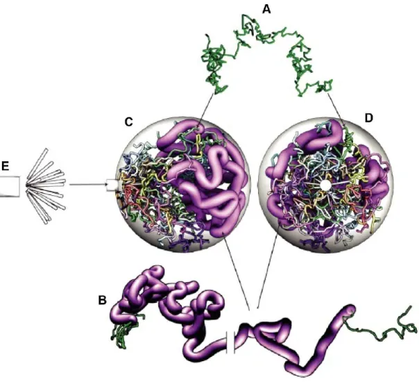
Figure 11. Computational model of the dynamic interphase yeast nucleus. From (Wong et al., 2012).
A. Each chromosome is modeled as a self-avoiding polymer with jointed rigid segments. B. The rDNA segment on chromosome XII is modeled by thicker segments (pink) than the non-rDNA (other colors).
C, D. A snapshot of the full model from different angle of views. E. The SPB and the 16 microtubules.
To statistically predict the positioning of any locus in the nuclear space, Wong et al. presented a computational model of the dynamic chromosome organization in the interphase yeast nucleus. In this model, the 16 chromosomes of haploid yeast were modeled as self-avoiding chains consisting of jointed rigid segments with a persistence length of 60 nm and a 20 nm
34
diameter (Figure 11A). All of the chromosomes were enclosed by a 1 μm radius sphere representing the nuclear envelope (Figure 11C, D) and their motion was simulated with Brownian dynamics, while respecting topological constraints within and between chains. This model also added constraints for three specific DNA sequences: CEN, TEL and the rDNA. Each CEN was tethered by a single microtubule to the SPB (Figure 11E). All the 32 TEL were anchored to the nuclear envelope. Considering the intense transcriptional activity of the rDNA, which leads to a strong accumulation of RNA and proteins at this locus, the diameter of the rDNA segments was considered larger than the 20 nm diameter assumed elsewhere (Figure 11B). Chromosome XII which contains the rDNA segments was therefore modeled as a copolymer.
This simple model accounted for most of the differences in average contact frequencies within and between individual chromosomes. It also performed well in predicting contact features at smaller genomic scales, down to roughly 50 kbp.
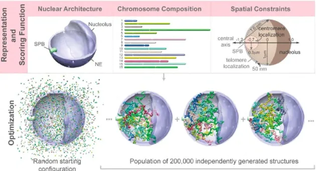
To determine which forces drive the positioning and clustering of functionally related loci in yeast, Gehlen et al. developed a coarse grained computational model (Gehlen et al., 2012). In this model, the chromosomes were modeled as coarse grained polymer chains and numerous constraints were implemented by users. Assuming that chromatin may exists at different compacted states (euchromatin and heterochromatin), at different locations within the genome of an individual cell, this model employs two different models to represent compact (30 nm diameter) and open (10 nm diameter) chromatin fibers. Compact chromatin was modeled as 30 nm fibers with a persistence length of 200 nm. Open chromatin was modeled as 10 nm fibers with a persistence length of 30 nm. Both types of chromatin fiber were used alternatively as part of the modeling of polymer chains in which 70% of the genome was compacted. This model allows to explore putative external constraints (nuclear envelope, tethering effects, and chromosome interactions).
Contact maps generated by 3C-technologies provide without any doubt the highest resolution dataset to constrain possible simulation of genome organization in vivo. Computational models allow to explore forces and constraints driving the folding of the genome in interphase nucleus. However, contact maps are mostly based on population analysis of asynchronous cell culture. Moreover, the impossibility to visualize the chromatin in individual cell nuclei and the difficulties to convert contact frequency to physical distances should not be ignored. Microscope-based techniques, combined with labeling methods to detect loci position and
35
motion offer important new perspectives for imaging genome structure. In the next part, I will present microscope-based techniques to study the spatial organization of chromosomes. 1.2.6 Gene position and gene territory
Fluorescence microscopy can fast acquire data and target molecules of interest with specific labeling strategies; therefore it has become an essential tool for biological research in vivo (Han et al., 2013). Thanks to the fluorescent labeling of chromosome loci in living cells, advanced imaging techniques can also provide considerable amount of data describing the spatial organization of single gene loci on chromosomes (Marshall et al., 1997). Fluorescent labeling of DNA sequences in living cells is mostly performed using fluorescent repressor-operator system (FROS) which combines the expression of a bacterial repressor fused to a fluorescent protein and the integration of an operator sequence as tandem arrays at a specific locus. A unique FROS tagged locus appears as a bright fluorescent spot in the nucleus (Loiodice et al., 2014; Meister et al., 2010) (Figure 12A).
The spatial resolution in fluorescence microscopy, 200 nm in X-Y and about 500 nm in Z-axis, is a barrier for high-resolution simultaneous detection of a large number of single molecules (Nelson and Hess, 2014). However, when single fluorescent molecules are spatially separated by more than the resolution limit of fluorescent microscopy, localization of their mass centers is only limited by signal-to-noise ratio. Such high precision of localization can be achieved by fitting pixel intensities spatially with the characteristic Gaussian distribution of fluorescence around local maxima. Therefore detection of the centroid of individual fluorescent molecules allows tracking the target with a resolution not limited by the diffraction of light (Thompson et al., 2002).
36
Figure 12. Nucloc to study the gene position.
A. The fluorescent repressor-operator system (FROS). Scale bar, 2 µm.
B. The yeast locus and the nuclear pores labeled in green and the nucleolus labeled in red. Nucloc can automatically detect the locations of a locus (green sphere), nuclear pores (blue spheres), nucleolar centroid (red sphere) and an estimated nuclear envelope. It enables to define a cylindrical coordinates system with an oriented axis in which we describe the position of the locus by its distance from the nuclear center (R) and the angle from the axis
37
nuclear-nucleolar centroid (α). The angle φ is defined by the angle around this axis, and is independent of the distances between the locus and the nuclear or nucleolar centroids. Nucloc uses nuclear center as the first landmark and translates all nuclear centers to the origin, and then rotated them around the origin so that nucleolar centroids (secondary landmark) became aligned on the X-axis. Then in these coordinates, the locus positions were rotated around the central axis and into a single plane (φ=0; cylindrical projection) without loss of information. From this 2D distribution of points, we could estimate the probability densities that are color coded on a genemap. Scale bars, 1 μm. Adapted from (Berger et al., 2008).
To analyze the spatial localization of a given locus in the yeast nucleus, Berger and colleagues created ‘Nucloc’ algorithm in which each cell nucleus of a population, determines the three dimensional position of a locus relative to the nuclear envelope, and the nuclear and nucleolar centers as landmarks (Berger et al., 2008). Automated detection allows high-throughput analysis of a large number of cells (>1000) automatically. The ‘Nucloc’ algorithm can create a high-resolution (30 nm) probability density map of subnuclear domains occupied by individual loci in a population of cells, thereby defining the domain in the nucleus in which a locus is confined: the ‘gene territory’ (Figure 12B) (Berger et al., 2008).
The genemap of specific loci, as well as 3C-techniques, can recover yeast chromosome organization in space compatible with their known features. The chromosome XII in budding yeast carries the ribosomal DNA (rDNA) confined in the nucleolus. Our group’s previous work analyzed 15 loci (12 non-rDNA loci and 3 rDNA loci) along chromosome XII by ‘Nucloc’. By comparing the maps, we could observe that loci around the CEN are attached to the SPB, at an opposite position of the nucleolus, the rDNA genes are clustered in the nucleolus, the TEL, are anchored to the NE. All these features are in agreement with the Rabl-like configuration and the recent computational models (Figure 13) (Albert et al., 2013; Duan et al., 2010; Tjong et al., 2012; Wong et al., 2012). We also assessed whether chromosome XII folding could be predicted by nuclear models based on polymer physics (Wong et al., 2012). The results showed that the measured median distance of loci on chromosome XII to the nuclear and nucleolar centers are compatible well with the model predictions (Figure 14 A,B) (Wong et al., 2012). However, we also should note that the fit to the model prediction was poorer for genomic positions 450-1050 kb, from the nucleolus to the right TEL (Figure 14 A, B).
38
Figure 13. The gene territories of 15 loci along chromosome XII. A. 15 FROS labeled loci along the chromosome XII.
B. Spatial distributions of each locus. The dashed yellow circle, the red circle, and the small red dot depict the median NE, the median nucleolus and the median location of the nucleolar center, respectively. From (Albert et al., 2013).
The gene territories can be remodeled during transcriptional activation. Based on this, we could study the gene motion during transcriptional activation. In glucose, the GAL1 gene is repressed and the gene positions indicate that the GAL1 gene concentrates in an intranuclear domain close to the nuclear center, whereas in galactose, GAL1 is actively transcribed and frequently re-localized to the nuclear periphery. This is consistent with the model where the on/off states of transcription correspond to two locations (Berger et al., 2008; Cabal et al., 2006). Recently, imaging entire chromosome II revealed global shift to nuclear periphery in
39
different physiological conditions modifying the yeast transcriptome (Dultz et al., 2016). Peripheral recruitment of chromosome arms strongly argues for transcription-dependent anchoring point along a chromosome (Tjong et al., 2012). Therefore, tethering sites organizing chromosomes locally remain to be identified (Dultz et al., 2016).
Figure 14. Positions of loci along the chromosome XII relative to the nuclear and nucleolar centers determined experimentally and predicted by computational modeling. From (Albert et al., 2013).
A, B. The distance of the locus to the nuclear center (A) and to the nucleolar center (B) is plotted versus its genomic position. Yellow and red ellipsoids represent the nuclear envelope and the nucleolus, respectively. The median distance experimentally measured is shown with box plots. The median distance of chromosome XII loci to the nuclear center and to the centroid of the rDNA segments from a computational model of chromosome XII is shown with solid black lines.