HAL Id: inria-00510392
https://hal.inria.fr/inria-00510392
Submitted on 18 Aug 2010
HAL is a multi-disciplinary open access
archive for the deposit and dissemination of
sci-entific research documents, whether they are
pub-lished or not. The documents may come from
teaching and research institutions in France or
abroad, or from public or private research centers.
L’archive ouverte pluridisciplinaire HAL, est
destinée au dépôt et à la diffusion de documents
scientifiques de niveau recherche, publiés ou non,
émanant des établissements d’enseignement et de
recherche français ou étrangers, des laboratoires
publics ou privés.
Multipitch estimation of piano sounds using a new
probabilistic spectral smoothness principle
Valentin Emiya, Roland Badeau, Bertrand David
To cite this version:
Valentin Emiya, Roland Badeau, Bertrand David. Multipitch estimation of piano sounds using a
new probabilistic spectral smoothness principle. IEEE Transactions on Audio, Speech and
Lan-guage Processing, Institute of Electrical and Electronics Engineers, 2010, 18 (6), pp.1643-1654.
�10.1109/TASL.2009.2038819�. �inria-00510392�
Multipitch estimation of piano sounds using
a new probabilistic spectral smoothness principle
Valentin Emiya, Member, IEEE, Roland Badeau, Member, IEEE, Bertrand David, Member, IEEE
Abstract—A new method for the estimation of multiple con-current pitches in piano recordings is presented. It addresses the issue of overlapping overtones by modeling the spectral envelope of the overtones of each note with a smooth autoregressive model. For the background noise, a moving-average model is used and the combination of both tends to eliminate harmonic and sub-harmonic erroneous pitch estimations. This leads to a complete generative spectral model for simultaneous piano notes, which also explicitly includes the typical deviation from exact harmonicity in a piano overtone series. The pitch set which maximizes an approximate likelihood is selected from among a restricted number of possible pitch combinations as the one. Tests have been conducted on a large homemade database called MAPS, composed of piano recordings from a real upright piano and from high-quality samples.
Index Terms—Acoustic signal analysis, audio processing, mul-tipitch estimation, piano, transcription, spectral smoothness.
I. INTRODUCTION
The issue of monopitch estimation has been addressed for decades by different approaches such as retrieving a periodic pattern in a waveform [1; 2] or matching a regularly spaced pattern to an observed spectrum [3–5], or even by combining both spectral and temporal cues [6; 7]. Conversely the mul-tipitch estimation (MPE) problem has become a rather active research area in the last decade [8–11] and is mostly handled by processing spectral or time-frequency representations. This MPE task has also become a central tool in musical scene analysis [11], particularly when the targeted application is the automatic transcription of music (ATM) [12–16]. While recent works consider pitch and time dimensions jointly to perform this task, MPE on single frames has been historically used as a prior processing to pitch tracking over time and musical note detection. Indeed, in a signal processing perspective, a period or a harmonic series can be estimated from a short signal snapshot. In terms of perception, only a few cycles are needed to identify a pitched note [17].
In this polyphonic context, two issues have proved difficult and interesting for computational MPE: the overlap between the overtones of different notes and the unknown number of such notes occurring simultaneously. As the superposition of two sounds in octave relationship leads to a spectral ambiguity
V. Emiya is with the Metiss team at INRIA, Centre Inria Rennes - Bretagne Atlantique, Rennes, France, and, together with R. Badeau and B. David, with Institut Télécom; Télécom ParisTech; CNRS LTCI, Paris, France.
The research leading to this paper was supported by the French GIP ANR under contract ANR-06-JCJC-0027-01, Décomposition en Éléments Sonores et Applications Musicales - DESAMand by the European Commission under contract FP6-027026-K-SPACE. The authors would also like to thanks Peter Weyer-Brown from Telecom ParisTech and Nathalie Berthet for their useful comments to improve the English usage.
and thus to an ill-posed problem, some knowledge is often used for the further spectral modeling of the underlying sources. For instance, when iterative spectral subtraction is em-ployed, several authors have adopted a smoothness assumption for the spectral envelope of the notes [8–10].
Several preceding works [12–14; 16] specifically address the case of the piano. One of the interests in studying a single instrument is to incorporate in the algorithms some results established from physical considerations [18; 19], in the hope that a more specific model will lead to a better performance, with the obvious drawback of narrowing the scope of the application. Indeed, while a large number of musical pieces are composed for piano solo, the performance of ATM systems is relatively poor for this instrument in comparison to others [6]. Two deviations from a simple harmonic spectral model are specific to free vibrating string instruments and are particularly salient for the piano: a small departure from exact harmonicity (the overtone series is slightly stretched) and the beatings be-tween very close frequency components (for a single string two different vibrating polarizations occur and the different strings in a doublet or triplet are slightly detuned on purpose [20]).
In this work, we propose a new spectral model in which the inharmonic distribution is taken into account and adjusted for each possible note. The spectral envelope of the overtones is modeled by a smooth autoregressive (AR) model, the smoothness resulting from a low model order. A smooth spectral model is similarly introduced for the residual noise by using a low-order moving-average (MA) process, which is particular efficient against residual sinusoids. The proposed method follows a preliminary work [21] in which the AR/MA approach was already used and MPE was addressed as an extension of a monopitch estimation approach. In addition to the opportunity to deal with higher polyphony levels, the current paper introduces a new signal model for simultaneous piano notes and a corresponding estimation scheme. The major advance from the previous study is thus to model and estimate the spectral overlap between note spectra. An iterative estimation framework is proposed which leads to a maximum likelihood estimation for each possible set of F0s.
This paper is structured as follows. In section II, the overall MPE approach is described. The sound model is first detailed, followed by the principle of the algorithm: statistical background, adaptive choice of the search space and detection function. The estimation of the model parameters is then explained in section III. After specifying the implementation details, the algorithm is tested in section IV using a database of piano sounds and the results are analyzed and compared with those obtained with some state-of-the-art approaches.
Conclusions are finally drawn in section V.
Note that in the following,∗denotes the complex conjugate, Tthe transpose operator,†the conjugate transpose, ⌊.⌋ the floor
function and |.| the number of elements in a set, the absolute value of a real number or the modulus of a complex number. In addition, the term polyphony will be applied to any possible mixture of notes, including silence (polyphony 0) and single notes (polyphony 1).
II. MULTIPITCH ESTIMATION ALGORITHM
A. Generative sound model
At the frame level, a mixture of piano sounds is modeled as a sum of sinusoids and background noise. The amplitude of each sinusoid is considered as a random variable. The spectral envelope for the overtone series of a note is introduced as second order statistical properties of this random variable, making it possible to adjust its smoothness. The noise is considered as a moving-average (MA) process.
More precisely, a mixture of P ∈ N simultaneous piano notes, observed in a discrete-time N-length frame, is modeled
as a sum x (t) , PP
p=1 xp(t) + xb(t) of the note
signals xp and of noise xb. The sinusoidal model for xp is
xp(t), Hp X h=1 ¡ αhpe2iπfhpt+ α∗hpe−2iπfhpt ¢ (1) where αhp are the complex amplitudes and fhp the
frequen-cies of the Hp overtones (here, Hp is set to the maximum
number of overtones below the Nyquist frequency). Note p is parameterized by Cp = (f0p, βp), f0pbeing the fundamental
frequency(F0) and βp(f0p) being the so-called inharmonicity
coefficientof the piano note [20], such that fhp, hf0p
q
1 + βp(f0p) h2 (2)
We introduce a spectral envelope for note p as an au-toregressive (AR) model of order Qp, parameterized by
θp , ¡σ2p, Ap(z)¢, where σp2 is the power and Ap1(z) is
the transfer function of the related AR filter. Order Qpshould
be low and proportional to Hp, in order to obtain a smooth
envelope and to avoid overfitting issues for high pitches. The
amplitude αhp of overtone h of note p is the outcome of a
zero-mean complex Gaussian random variable1, with variance
equal to the spectral envelope power density at the frequency fhp of the overtone: αhp∼ N Ã 0, σ 2 p |Ap(e2iπfhp)| 2 ! (3) In order to model a smooth spectral envelope without residual peaks, the noise xb is modeled as an MA process
with a low order Qb, parameterized by θb ,
¡ σ2 b, B(z) ¢ , σ2 b
being the power and B(z) the finite impulse response (FIR) filter of the process.
Furthermore, high note powers and low noise powers are favored by choosing an inverse gamma prior for σ2
p: 1Using these centered Gaussian variables, x
pis thus a harmonic process, in the statistical sense.
Pr ep ro ce ss in g Pa ra m et er es ti m at io n D ec is io n
For each possible mixture C
Frame:(x (0) , . . . , x (N − 1))T
Selection of mixture candidates Preprocessing
Iterative estimation of note models
p∈ J1; P K Amplitude estimation Weighted log-likelihood ˜Lx(C) C ∈ eC Spectral envelope AR parameter estimation Noise MA parameter estimation Mixture estimation: bC arg maxC∈ eCL˜x(C)
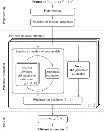
Fig. 1. Multipitch estimation block diagram.
σ2 p ∼ IG ³ kσ2 p, Eσ2p ´
and a gamma prior for σ2 b: σ2b ∼ Γ³kσ2 b, Eσ 2 b ´
. A non-informative prior2is assumed for A p(z)
and B(z).
With a user-defined weighting window w, we can equiv-alently consider the Discrete Time Fourier Transforms (DTFT) Xp(f ) of xp(t) w (t), Xb(f ) of xb(t) w (t) and
X (f ) , PP
p=1 Xp(f ) + Xb(f ) of x (t) w (t). W being
the DTFT of w, we thus have Xp(f ) = Hp X h=1 ¡ αhpW (f − fhp) + α∗hpW∗(f + fhp) ¢ (4) In addition, the following synthetic notations will be used: a mixture of notes is denoted by C , (C1, . . . , CP); the set of
parameters for spectral envelope models by θ , (θ1, . . . , θP);
the set of amplitudes of overtones of note p by αp ,
¡
α1p, . . . , αHpp
¢; and the set of amplitudes of overtones of all notes by α , (α1, . . . , αP).
B. Principle of the algorithm
The algorithm is illustrated in Fig. 1. The main principles are described in the current section, except for the model parameter estimation, which is detailed in Section III.
2e.g.an improper, constant prior density, which will not affect the detection function.
1) Statistical background: Let us consider the observed frame x and the set C of all the possible mixtures of pia-no pia-notes. Ideally, the multipitch detection function can be expressed as the maximum a posteriori (MAP) estimator ˆC, which is equivalent to the ML estimator if no a priori information on mixtures is specified:
ˆ C = arg max C∈C p(C|x) = arg max C∈C p(x|C) p(C) p(x) = arg max C∈C p(x|C) (5)
2) Search space: The number of combinations among Q possible notes being ¡Q
P
¢ for polyphony P , the size of the search set C is PQ
P=0
¡Q P
¢
= 2Q, i.e. around 3·1026 for a
typical piano with Q = 88 keys. Even when the polyphony is limited to Pmax= 6 and the number of possible notes to Q =
60 (e.g. by ignoring the lowest and highest-pitched keys), the number of combinations reaches PPmax
P=0
¡Q P
¢
≈ 56·106, which
remains a too huge search set for a realistic implementation. In order to reduce the size of this set, we propose to select a given number Nc of note candidates. We use the normalized
product spectrum function defined in dB as ΠX(f0, β), 1 H (f0, β)ν10 log H(f0,β) Y h=1 |X (fh)|2 (6)
where X is the observed spectrum, H (f0, β) is the number
of overtones for the note with fundamental frequency f0 and
inharmonicity β, fh , hf0
p
1 + βh2, and ν is a parameter
adjusted to balance the values of the function between bass and treble notes. As the true notes generate local peaks in ΠX,
selecting an oversized set of Nc greatest peaks is an efficient
way for adaptively reducing the number of note candidates. In addition, for candidate nc∈ J1; NcK, accurate values of its
fundamental frequency f0nc and inharmonicity βnc are found
by a local two-dimensional maximization3 of Π
X(f0nc, βnc).
They are used in the subsequent estimation stages to locate the frequencies of the overtones. In the current implementation, the number of note candidates is set to Nc = 9. This choice
results from the balance between increasing the number of candidates and limiting the computational time. The size of the set eCof possible mixtures thus equalsPPmax
P=0 ¡Nc P ¢ = 466, for Pmax= 6.
3) Multipitch detection function: The multipitch detection function aims at finding the correct mixture among all the possible candidates. For each candidate C ∈ eC, the parameters
b
α, bθ and bθb of the related model are estimated as explained
in section III. The detection function is then computed, and the multipitch estimation is defined as the mixture with the greatest value.
Since equation (5) is intractable, we define an alternate detection function which involves the following terms:
• Lp(θp) , ln p(αp|θp, Cp) is the log-likelihood of the
amplitudes αp of overtones of note p, related to the
spectral envelope models θp;
3The fminsearch Matlab function was used for this optimization.
• Lb(θb), ln p(x|α, θb, C) is equal4 to the log-likelihood
ln pxb related to the noise model θb;
• the priors ln p(θp) on the spectral envelope of the note p
and ln p(θb) on noise parameters.
We empirically define the detection function as a weighted sum of these log-densities, computed with the estimated pa-rameters (see Appendix A for a discussion):
˜ Lx(C), w1 P X p=1 ˜ Lp ³ b θp ´ /P + w2L˜b ³ b θb ´ + w3 P X p=1 ln p³cσ2 p ´ /P + w4ln p ³ c σ2 b ´ − µpolP (7) where ˜ Lp ³ b θp ´ , 1 HpLp ³ c σ2 p, cAp ´ − µenvHp ˜ Lb ³ b θb ´ , 1 |Fb|Lb ³ c σ2 b, bB ´ − µb |Fb|
w1, . . . , w4, µpol, µenv, µb are user-defined
coefficients
|Fb| is the number of noisy bins (see eq. (14)).
III. MODEL PARAMETER ESTIMATION
A. Iterative estimation of spectral envelope parameters and amplitudes of notes
We consider a possible mixture C = (C1, . . . , CP). The
estimation of the unknown spectral envelope parameters θ and of the unknown amplitudes of the overtones α is performed by iteratively estimating the former and the latter, as described in this section.
1) Spectral envelope parameter estimation: let us assume the amplitudes α are known in order to estimate the spectral envelope parameters θ in the maximum likelihood (ML) sense. Given that note models are independent, the likelihood of α is p(α|θ, C) = QP
p=1p(αp|θp, Cp). The optimization w.r.t. θ
thus consists in maximizing the log-likelihood Lp¡σ2p, Ap¢,
ln p¡αp|σp2, Ap, Cp ¢ w.r.t. θp = ¡ σ2 p, Ap ¢ , independently for each note p. As proved in the Appendix B, the maximization w.r.t. σ2
p leads to the expression
Lp ³ c σ2 p, Ap ´ = c + Hp 2 ln ρ (Ap) (8) with c, −Hp 2 ln (2πe) − 1 2 Hp X h=1 ln |αhp|2 (9) ρ (Ap), ³QHp h=1|αhp|2 ¯ ¯Ap¡e2iπfhp¢¯¯ 2´Hp1 1 Hp PHp h=1|αhp|2|Ap(e2iπfhp)|2 (10) c σ2 p= 1 Hp Hp X h=1 |αhp|2 ¯ ¯Ap¡e2iπfhp¢¯¯ 2 (11)
4by using the substitution x 7→ x − 2Re“PP p=1
PHp
h=1αhpe2iπfhpt ”
, t being the time instants related to the frame, this term is equal to lnpxb “ x − 2Re“PP p=1 PHp h=1αhpe2iπfhpt ” |θb ”
0 2000 4000 6000 8000 10000 −20 0 20 40 f (Hz) dB ln ρ³Ac1 ´ = −0.47 |X(f)|2/N ˆ θ1 |ˆαh1|2
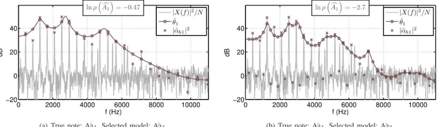
(a) True note: A♭4. Selected model: A♭4.
0 2000 4000 6000 8000 10000 −20 0 20 40 f (Hz) dB ln ρ³Ac1 ´ = −2.7 |X(f)|2/N ˆ θ1 |ˆαh1|2
(b) True note: A♭4. Selected model: A♭3.
Fig. 2. Estimation of spectral envelopes: the AR estimation performs a better fitting of the amplitudes for the correct model (left) than for the sub-octave model (right).
As c is a constant w.r.t. Ap, the optimization consists in
maximizing ρ (Ap), which measures the spectral flatness (i.e.
the ratio between the geometrical and arithmetical means) of n |αhp|2 ¯ ¯Ap ¡ e2iπfhp¢¯¯2 o 1≤h≤Hp
. This quantity lies in [0; 1] and is maximum when the latter coefficients are constant, i.e. when the filter Ap perfectly whitens the amplitudes αp. The
estimation of Apfrom the discrete data αpthanks to the Digital
All-Pole (DAP) method [22] leads to a solution that actually maximizes ρ (Ap), as proved in [23]. It is applied here to the
amplitudes αp, for each note p.
The estimation of the spectral envelope of a note is il-lustrated in Fig. 2. A note is analyzed by considering two possible models: the model related to the true note (Fig. 2(a)) and the model related to its sub-octave (Fig. 2(b)). In the former case, the estimate of the spectral envelope is close to the amplitudes of the overtones, whereas in the latter case, the AR spectral envelope model is not adapted to amplitudes that are alternatively high and low: the low values obtained for the spectral flatness ρ (and, consequently, for the likelihood) are here a good criterion to reject wrong models like the sub-octave (see Fig. 6(a) for the whole spectral flatness curve).
2) Estimation of the amplitudes of the overtones: let us now assume that spectral envelope parameters θ are known, that the frequencies of the overtones may overlap, and that the amplitudes α are unknown. In all that follows, we assume that at a given overtone frequency fhp, the power spectrum
of the noise is not significant in comparison with the power spectrum of the amplitudes of the overtone.
When the overtone h of note p is not overlapping with any other overtone, the amplitude αhp is directly given by the
spectrum value X (fhp). In the alternative case of overlapping
overtones, the observed spectrum results from the contribution of overtones with close frequencies. We propose an estimate of the hidden random variable α, given the observation X and the parameters θ that control the second-order statistics of α. As defined by eq. (3), the amplitude αhp is a random
vari-able such that αhp ∼ N (0, vhp) with vhp ,
σ2 p
|Ap(e2iπfhp)| 2.
One can rewrite the sound model x as a sum of K sinusoids and noise x(t) =PK
k=1αke2iπfkt+xb(t) with αk ∼ N (0, vk)
and K = 2PP
p=1Hp. In this formula, the couples of indexes
(h, p) related to overtones and notes have been replaced by
a single index k. In the spectral domain, the DFT X of the N -length frame x using a weighting window w of DFT W is X (f) = PK
k=1αkW (f − fk), the noise spectrum being
removed since we are only interested in the values of X at frequencies fhp, where the noise term is insignificant.
In these conditions, for 1 ≤ k0 ≤ K, the optimal linear
estimator ˆαk0 of αk0 as a function of X (fk0), obtained by
minimizing the mean squared error ǫk0 = E
h |αk0− ˆαk0| 2iis ˆ αk0 = W∗(0) v k0 PK k=1|W (fk0− fk)| 2 vk X (fk0) (12)
The proof of eq. (12) is given in the Appendix B. By ignoring non-overlapping overtones, the expression of the estimator of αhp can be simplified as
d αhp , W∗(0) v2 hp P |fh′ p′−fhp|<∆w |W(fh′ p′−fhp)| 2 v2 h′ p′ X (fhp) (13)
where ∆w is the width of the main lobe of W .
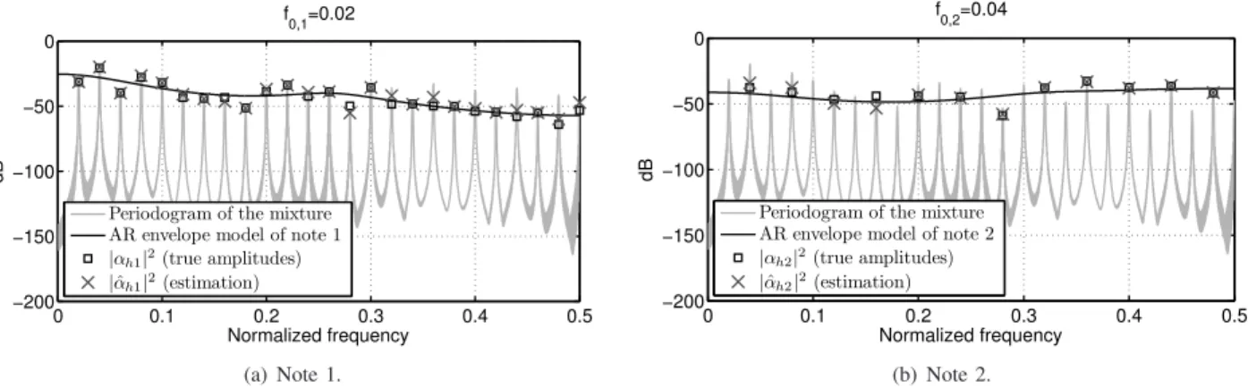
The amplitude estimation is illustrated in Fig. 3 on a synthetic signal, composed of two octave-related notes, i.e. with overlapping spectra. As expected, the amplitudes are perfectly estimated when there is no overlap (see odd-order peaks of note 1). When the overtones overlap, predominant amplitudes are well estimated (see note 1 for f = 0.04 or note 2 for f = 0.4), as well as amplitudes with the same order of magnitude (see amplitudes at f = 0.2). The estimation may be less accurate when an amplitude is much weaker than the other (see note 1 at f = 0.36).
3) Iterative algorithm for the estimation of note parameters:
in the last two parts, we have successively seen how to estimate the spectral envelope models from known amplitudes and the amplitudes from known spectral envelope models. None of these quantities are actually known, and both must be estimated. We propose to use the two methods above in the Algorithm 1 to iteratively estimate both the spectral envelope and the amplitudes of the overtones. It alternates the estimation of the former and of the latter, with an additional thresholding of the weak amplitudes in order to avoid the amplitude estimates becoming much lower than the observed
0 0.1 0.2 0.3 0.4 0.5 −200 −150 −100 −50 0 Normalized frequency dB f 0,1=0.02
Periodogram of the mixture AR envelope model of note 1 |αh1|2(true amplitudes) |ˆαh1|2(estimation) (a) Note 1. 0 0.1 0.2 0.3 0.4 0.5 −200 −150 −100 −50 0 Normalized frequency dB f 0,2=0.04
Periodogram of the mixture AR envelope model of note 2 |αh2|2(true amplitudes)
|ˆαh2|2(estimation)
(b) Note 2.
Fig. 3. Estimation of amplitudes from overlapping spectra: example on a synthetic mixture of 2 notes. The F0s f0,1 and f0,2of the two notes are in an octave relation and the estimation is performed from a N = 2048-length observation. For each note, the true amplitudes (squares) have been generated from a spectral envelope AR model (black line) using eq. (3). The amplitudes are estimated (crosses) from the observation of the mixture (grey line) using the AR envelope information (eq. (12)).
0 2000 4000 6000 8000 10000 −30 −20 −10 0 10 20 30 40 50 60 f (Hz) dB |X|2/N ˆ θ1 ˆ αh1 ˆ θ2 ˆ αh2
(a) True notes: G5+D6. Selected model: G5+D6.
0 2000 4000 6000 8000 10000 −30 −20 −10 0 10 20 30 40 50 60 f (Hz) dB |X|2/N ˆ θ1 ˆ αh1 ˆ θ2 ˆ αh2
(b) True notes: F#4+F#5. Selected model: F#4+F#5. Fig. 4. Iterative estimation of amplitudes cαpand spectral envelopes bθp: example of a fifth (Fig. 4(a)) and of an octave (Fig. 4(b)).
spectral coefficients5. For p ∈ J1; P K and h ∈ J1; H pK, the
estimate dαhp of αhp and bθp of θp are respectively the values
of ³α(i)hp´and ³θ(i)p
´
after a number of iterations. Note that the ML estimates of the envelopes are directly related to the MAP estimation of the multipitch contents while amplitudes are estimated in the least mean square sense, which is a different objective function. Consequently, the convergence of the iterative algorithm is not proved or guaranteed but it is observed after about Nit, 20 iterations.
The estimation is illustrated in Fig. 4 with two typical cases. While the energy is split between the overlapping overtones, non-overlapping overtones help estimating the spec-tral envelopes, resulting in a good estimation in the case of a fifth (Fig. 4(a)), the octave being a more difficult – but successful – case (Fig. 4(b)).
B. Estimation of noise parameters
We assume that the noise signal results from the circular filtering6of a white centered Gaussian noise with variance σ2 b
5In our implementation, this threshold was set to the minimum observed amplitude minf |X(f )|√N .
6The circularity assumption, which is commonly used and asymptotically valid, leads to a simplified ML solution.
Algorithm 1 Iterative estimation of note parameters Require: spectrum X, notes C1, . . . , CP.
Initialize the amplitudes α(0)hp of overtones to spectral values X (fhp) for p ∈ J1; P K and h ∈ J1; HpK.
foreach iteration i do foreach note p do
Estimate θ(i)
p from α(i−1)p . {AR estimation}
end for
Jointly estimate all α(i)
hpfrom X (fhp) and θp(i). {eq. (13)}
Threshold α(i)hp at a minimum value. end for
Ensure: estimation of αhp and θp for p ∈ J1; P K and h ∈
J1; HpK.
by a Qb-order FIR filter parameterized by its transfer function
B (z) =PQb
k=0bkz−k, with b0= 1.
As we assumed that in a bin close to the frequency of an overtone, the spectral coefficients of noise are negligible w.r.t. the spectral coefficients of notes, the information related to noise is mainly observable in the remaining bins, i.e. on the
0 2000 4000 6000 8000 10000 −40 −20 0 20 40 60 f (Hz) d B ln ρb ³ b B´= −1.3 X(Fb) X(Fb) MA estimation ˆθb
(a) True note: E♭4. Selected model: E♭4.
0 2000 4000 6000 8000 10000 −40 −20 0 20 40 60 f (Hz) d B ln ρb ³ b B´= −3.6 X(Fb) X(Fb) MA estimation ˆθb
(b) True note: E♭4. Selected model: E♭5. Fig. 5. Noise parameter estimation when selecting the true model (left) and the octave model (right). Fbdenotes the complement of Fb.
frequency support defined by Fb, ½ k Nfft Á ∀p ∈ J1; P K, ∀h ∈ J1; HpK, ¯ ¯ ¯ ¯Nkfft−fhp ¯ ¯ ¯ ¯ >∆2w ¾ (14) where ∆wdenotes the width of the main lobe of w (∆w= N4
for a Hann window) and Nfftis the size of the DFT. The noise
parameter estimation is then performed using this subset of bins, which gives satisfying results asymptotically (i.e. when N → +∞, the number of removed bins being much smaller than the total number of bins). As proved in the Appendix B, it results in the maximization, w.r.t. B, of the expression
Lb ³ c σ2 b, B ´ = cb+ |Fb| 2 ln ρb(B) (15) where cb, − |Fb| 2 ln 2πe − 1 2 X f∈Fb ln|Xb(f )| 2 N (16) ρb(B), µ Q f∈Fb ¯ ¯ ¯ Xb(f ) B(e2iπf) ¯ ¯ ¯ 2¶|Fb1| 1 |Fb| P f∈Fb ¯ ¯ ¯ Xb(f ) B(e2iπf) ¯ ¯ ¯2 (17) c σ2 b = 1 |Fb| X f∈Fb 1 N ¯ ¯ ¯ ¯B (eXb2iπf(f )) ¯ ¯ ¯ ¯ 2 (18) As for the spectral envelope AR parameters (eq. (11) and (8)), the ML estimation of noise parameters consists in the maximization of a spectral flatness ρb(B). It can be
achieved thanks to the MA estimation approach proposed in [23]. However, in order to speed up the computations, we use the Algorithm 3 described in the Appendix C, which is simpler and gives satisfying results for the current application. The noise parameter estimation is illustrated in Fig. 5. When the true model is selected (Fig. 5(a)), most of primary lobes of the sinusoidal components are removed from Fb
and the resulting spectral coefficients are well-fitted by an MA envelope. In the case a wrong model is selected and a lot of Fb bins are related to sinusoids (Fig. 5(b)), the MA
model is not adapted to the observations which are not well-fitted. The resulting ρb value and likelihood will be low so
40 50 60 70 80 90 −4 −3 −2 −1 0 note (MIDI) ln(ρ(A1)) True note + −octave (a) ln ρ“Acp ” . 40 50 60 70 80 90 −5 −4 −3 −2 −1 note (MIDI) ln(ρb) True note + −octave (b) ln ρb “ b B”. Fig. 6. ln ρ“Ac1 ” (top) and ln ρb “ b
B”(bottom) as a function of a single-note model (true single-note: A♭4).
that the wrong model will be rejected. As shown in Fig. 6, the spectral flatness criterion for the spectral envelope and noise estimations are complementary cues for rejecting wrong models and selecting the right one. The criterion on spectral envelopes (Fig. 6(a)) shows many high values but also large minima for sub-harmonic errors (e.g. notes D♭3, A♭3 and
D♭3 in this example). Conversely, the criterion for the noise
model (Fig. 6(b)) has a few high peaks located at the sub-harmonics F0s of the true note – i.e. for every model all the
sinusoids have been removed from the noise observation –, but is efficient for discriminating the other errors. Thus, if taken separately, these criteria are not good pitch estimators, but they efficiently combine into the detection function.
IV. EXPERIMENTAL RESULTS
A. Implementation and tuning
The whole method is summarized by Algorithm 2. The MPE algorithm is implemented in Matlab and C. It is designed to analyze a 93ms frame and to estimate its polyphonic content. A preprocessing stage aims at reducing the spectral dynamics and consists in flattening the global spectral decrease by means of a median filtering of the spectrum. The values of the parameters of the MPE algorithm are given in Table I. The order Qp of the spectral envelope filter Ap(z) of a note
p is set to Qp = Hp/2 in order to be large enough to
fit the data and small enough to obtain a smooth spectral envelope7. Parameters³k σ2 p, Eσ2p ´ ,³kσ2 b, Eσ 2 b ´ , µenv, µb, µpol
and (w1, . . . , w4) have been estimated on a development
database composed of about 380 mixtures from two different pianos, with polyphony levels from 1 to 6. They were jointly adjusted by optimizing the F-measure using a grid search, the bounds of the grid being set by hand.
Algorithm 2 Multipitch estimation. Preprocessing
Computation of periodogram 1 N |X|
2
Selection of Nc note candidates
foreach possible note combination C do
Iterative estimation of the amplitudes of overtones and of spectral envelope of notes (algorithm 1)
For each note p, derivation of Lp (eq. (8)) and of prior
p³cσ2 p
´
Noise parameter estimation (algorithm 3) Computation of Lb (eq. (15)) and of prior p
³ c σ2 b
´ Derivation of the detection function related to the note combination (eq. (7))
end for
Maximization of the detection function
Parameter value Parameter value Pmax 6 “kσ2 p, Eσ2p ” ` 1, 10−4´ Nc 9 “ kσ2 b, Eσ 2 b ” ` 2, 10−3´ ν 0.38 µenv −8.9·10−3 fs 22050Hz µb −2.2·10−4 N 2048 µpol 25 w Hann w1 8.1·10−1 Qp Hp/2 w2 1.4·104 Qb 20 w3 6.2·102 Nit 20 w4 5.8 TABLE I
PARAMETERS OF THE ALGORITHM.
B. Evaluation
The proposed MPE algorithm has been tested on a database called MAPS8 and composed of around 10000 piano sounds
7Note that the number of degrees of freedom for the AR models is H p/4 = Qpsince half the poles are affected to the positive frequencies, the remaining poles being their complex conjugates.
8MAPS stands for MIDI Aligned Piano Sounds and is available on request.
either recorded by using an upright Disklavier piano or generated by several virtual piano software products based on sampled sounds. The development set and the test set are disjointed. Two pianos are used in the former while the latter comprises sounds from other five pianos. In total, two upright pianos and five grand pianos were used. Recording conditions and tunings vary from one instrument to the other. Polyphony levels lie between 1 and 6 and notes are uniformly distributed between C2 (65Hz) and B6 (1976Hz). One part
of the polyphonic mixtures is composed of randomly related pitches whereas the other part comprises usual chords from western music (major, minor, etc.). For each sound, a single 93ms-frame located 10ms after the onset time is extracted and analyzed. Two additional algorithms have been tested on the same database for comparison purposes. The first one is Tolo-nen’s multipitch estimator [24] for which the implementation from the MIR Toolbox [25] was used. As the performance of the algorithm decreases when F0s are greater than 500Hz (C5),
the system was additionally tested in restricted conditions – denoted Tolonen-500 – by selecting from the database the subset of sounds composed of notes between C2 and B4only.
The second one is Klapuri’s system [26]. The code of the latter was provided by its author.
Our algorithm was implemented in Matlab and C. The com-putational cost on a recent PC is about 150×real time. It thus requires more computations than other algorithms like [26] but the proposed algorithm is computationally tractable, par-ticularly when comparing it to the greedy and intractable joint-estimation approach where no note candidate selection is performed, as discussed in section II-B.
General results are presented in Fig. 7. Relevant items are defined as correct notes after rounding each F0 to the
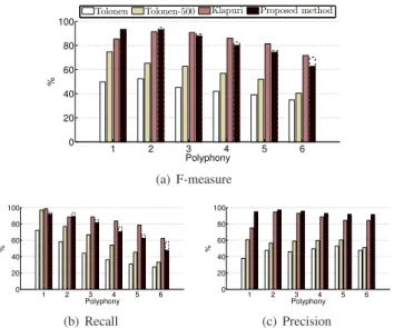
nearest half-tone. Typical metrics are used: the recall is the ratio between the number of relevant items and of original items; the precision is the ratio between the number of relevant items and of detected items; and the F-measure is the harmonic mean between the precision and the recall. In this context, our system performs the best results for polyphony 1 and 2: 93% F-measure vs 85% (polyphony 1) and 91% (polyphony 2) for Klapuri’s system. The trend then reverses between Klapuri’s system and the proposed one, the F-measure being respectively 91% and 88% for polyphony 3, and 72% and 63% for polyphony 6. Moreover, the precision is high for all polyphony levels whereas the recall is decreasing when polyphony increases. Results from Tolonen’s system are weaker for the overall tests, even with the restricted F0-range
configuration.
The ability of Klapuri’s system and ours to detect polyphony levels (independently of the pitches) is presented in Tab. II. For polyphony levels from 1 to 5, both systems succeed in detecting the correct polyphony level more often than any other level. It should also be noted that the proposed system was tested in more difficult conditions since polyphony 0 (i.e. silence) may be detected, which is the case for a few sounds9.
The proposed system tends to underestimate the polyphony
9Note that silence detection could be improved by using an activity detector as a preprocessing stage, since silence is a very specific case of signal that can be detected using more specific methods than the proposed one.
1 2 3 4 5 6 0 20 40 60 80 100 Polyphony %
Tolonen Tolonen-500 Klapuri Proposed method
(a) F-measure 1 2 3 4 5 6 0 20 40 60 80 100 Polyphony % (b) Recall 1 2 3 4 5 6 0 20 40 60 80 100 Polyphony % (c) Precision
Fig. 7. Multipitch estimation results with unknown polyphony: for each algorithm, the F-measure, the precision and the recall are rendered as a function of the true polyphony. For the proposed method, the performance on the training set is plotted using a dashed line.
P Pest 1 2 3 4 5 6 0 7 2 4 6 9 0 1 90 14 8 8 8 12 2 3 83 18 12 8 19 3 0 1 68 27 16 25 4 0 0 2 47 27 32 5 0 0 0 1 31 11 6 0 0 0 0 1 1 P Pest 1 2 3 4 5 6 0 0 0 0 0 0 0 1 92 21 5 2 1 3 2 1 74 18 7 4 7 3 1 3 65 24 10 12 4 0 1 9 49 24 27 5 1 0 1 14 36 23 6 5 1 1 4 25 28
Proposed method Klapuri’s method TABLE II
POLYPHONY ESTIMATION:DETECTION RATE(%)W.R.T.TO THE NUMBER OF SOUNDS WITH TRUE POLYPHONYP ,AS A FUNCTION OF THE TRUE
POLYPHONYPAND OF THE ESTIMATED POLYPHONYPEST.
level since the parameter tuning consists in optimizing the F-measure on the development set. This objective function could have been changed to take the polyphony level balance into account. This would result in reducing the polyphony underestimation trend. However, the overall F-measure would decrease. From a perceptive point of view, it has been shown that a missing note is generally less annoying than an added note when listening to a resynthesized transcription [27]. Thus, underestimating the polyphony may be preferred to overestimating it. Still, this trend turns out to be the main shortcoming of the proposed method, and should be fixed in the future for efficiently addressing sounds with polyphony higher than 5 notes.
The case of octave detection has been analyzed and results are presented in Fig. 8. Octave detection is one of the most difficult cases of multipitch estimation and the results are lower than the global results obtained for polyphony 2 (see Fig. 7). The proposed method reaches the highest results here, the F-measure being 81%, versus 77% for Klapuri’s system and 77%/66% for Tolonen’s (depending on the two F0 ranges).
This would suggest that the proposed models for spectral envelopes and overlapping spectra are significatively efficient.
Recall Precision F−measure 0 20 40 60 80 100 % Octave detection
Tolonen Tolonen-500 Klapuri Proposed method
Fig. 8. Octave detection: results for the 97 octave sounds extracted from the database (45 sounds for the Tolonen-500 system).
Finally, we report additional results which are not depicted. First, if polyphony is known, the performance of our sys-tem reaches the second rank after Klapuri’s syssys-tem, with correct detection rates from 95% (polyphony 1) down to 55% (polyphony 6). Second, F-measure values are between 5% and 10% better for usual chords than for random-pitch chords. This has been observed with all the tested methods for polyphony levels higher than two. While the algorithms face more harmonically-related notes in usual chords – i.e. more spectral overlap –, it seems that simultaneous notes with widely-spread F0s in random chords are a bigger difficulty.
Third, the results obtained on the development set and the test set are comparable, with only a few % deviation. This shows that the parameter learning is not overfitting and that the system has good generalization abilities for other models of piano and different recording conditions. Fourth, the whole database includes sounds from seven different pianos. The results are comparable from one piano to the other, with about 3%-standard deviation. Results do not significantly depend on the upright/grand piano differences, on recording conditions or on whether a real piano or a software-based one is used, which suggests robustness for varying production conditions. Fifth, the proposed method uses a candidate selection stage which may fail, causing the subsequent multipitch estimation to fail. The performance of the candidate selection stage has thus been checked: satisfying results are obtained for low to medium polyphony levels, 99% of true notes being selected for polyphony 1 and 2, 94% for polyphony 3 and 86% for polyphony 4. Performance is slightly decreasing in polyphony 5 and 6, the scores being 78% and 71% respectively. Along the original-pitch dimension, these errors are mainly located below A2(110Hz), and above A6(1760Hz). Selecting a set of likely
F0s is a challenging issue for future works since a lot of MPE
algorithms would benefit from it. Indeed, they often consist in optimizing an objective criterion that presents a lot of local optima along the pitch dimension. Some basic solutions like exhaustive or grid search [27] or more elaborated ones like Markov chain Monte Carlo methods [28] have already been proposed for searching the global optimum, and an efficient candidate selection stage would be very helpful to reach the result more quickly.
C. Integration in an automatic transcription system
The proposed MPE method has been introduced for a single-frame analysis. Beyond the multipitch issue, the automatic transcription task is addressed by integrating this method in
a system that performs pitch tracking over time and outputs not only pitches but note events. In the current case, the MPE method can be used in the transcription framework proposed in [19]. The automatic transcription of piano music is thus obtained by:
1) using an onset detector to localize new events; 2) detecting a set of pitch candidates after each onset; 3) between two consecutive onsets, decoding the multipitch
contents thanks to a frame-based Hidden Markov Model (HMM), the states being the possible combinations of simultaneous pitches, the likelihood being given by the proposed MPE method (eq. (7));
4) postprocessing the decoded pitches to detect repetitions or continuations of pitches when an onset occurs. This transcription system was presented at the Multiple
Fundamental Frequency Estimation & Tracking task of the MIREX10 contest in 2008 (system called EBD2). For the
piano-only test set, the evaluation is performed in two different ways, depending on how a correct note is defined. In the first, more constraining evaluation, where a correct note implies a correct onset (up to a 50-ms deviation), a correct offset (up to a 20%-duration or 50-ms deviation) and a correct pitch (up to a quartertone deviation), the proposed system reaches the 3rd rank with a 33.1% F-measure, out of 13 systems
scoring from 6.1% to 36.8%. For that evaluation, the duration estimation is evaluated by the average overlap between correct estimations and reference notes: the proposed method reaches the 7thposition with 80%, the values being in a narrow interval
([77.4%; 84%]). In the second evaluation, where correctness only requires the onset and pitch criteria above, the proposed system reaches the 7th rank with a 56.9% F-measure, out of
13 systems scoring from 24.5% to 75.7%. The best rank is obtained for average overlap with a 61% value, the lowest value being 40.1%.
Thus, when the proposed MPE method is integrated in a full transcription system for piano music, state-of-the art results are reached in terms of global performance. In addition, good average overlap scores show that the proposed method is suitable for pitch tracking over time and note extraction.
Note that one can wonder whether the reported performance is significant when comparing MPE and ATM quantitative results (with roughly 20% F-measure deviation, no matter the method is). It actually depends not only on the database, but on the different testing protocols. While isolated frames com-posed of one chord are used in the procom-posed MPE evaluation, ATM evaluation implies other difficulties like having asyn-chronous notes overlaping in time; detecting onsets; estimating the end of damping notes; dealing with reverberation queues and so on. More, polyphony levels in musical recordings are often high and are not uniformly distributed at all, with a 4.5 average polyphony and a 3.1 standard deviation reported for a number of classical music pieces [29, p.114]. Hence, F-measure for MPE and ATM should be evaluated separately.
10http://www.music-ir.org/mirex/2008/
V. CONCLUSIONS
In this paper, a sound model and a method were proposed for the multipitch estimation problem in the case of piano sounds. The approach was based on an adaptive scheme, including the adaptive matching of the inharmonic distribution of the frequencies of the overtones and an autoregressive spectral envelope. We have shown the advantage of using a moving average model for the residual noise. The estimation of the parameters was performed by taking the possible overlap between the spectra of the notes into account. Finally, a weighted likelihood criterion was introduced to determine the estimated mixture of notes in the analyzed frame among a set of possible mixtures.
The performance of the method was measured on a large database of piano sounds and compared to the state-of-the-art. The proposed method provides satisfying results when polyphony is unknown, and reaches particularly good scores for mixtures of harmonically-related notes.
This approach has been successively integrated in a full transcription system [19] and alternative investigations [30] are ongoing. Future works may deal with the use of differ-ent spectral envelopes in a similar modeling and estimation framework. Indeed, while the proposed AR envelope model may be too generic to characterize the spectral envelope smoothness of musical instruments, this information can be easily replaced, as the variance of the amplitude Gaussian models, by any parametric envelope model. The method may also be extended to other instruments or to voice. Keeping the proposed sound model, it could be useful to investigate other estimation strategies in order to reduce the computational cost. This may be achieved by means of a hybrid approach with an iterative selection of the notes and a joint estimation criterion. Furthermore, the log-likelihood function related to the model for spectral envelopes is not very selective. Hence, some investigations on more appropriate functions could improve the performance of decision step. Finally, one could conduct others investigations about how to prune the set of all possible note combinations more efficiently. They may include iterative candidate selection or MCMC methods.
APPENDIXA
DISCUSSION ON THE DETECTION FUNCTION
According to eq. (5), the multipitch estimation is theoreti-cally obtained by maximizing, w.r.t. C, the likelihood p(x|C), which is expressed as a function of the parameters of the proposed model as:
p(x|C) = ZZ p(x, α, θb|C) dαdθb (19) = ZZ p(x|α, θb, C) p(α|C) p(θb) dαdθb (20) = ZZZ p(x|α, θb, C) p(α|θ, C) p(θ) p(θb) dθdαdθb (21) Since the derivation of eq. (21) is not achievable, a simpler detection function must be built. The proposed function can be interpreted as a weighted log-likelihood and is obtained from the integrand of eq. (21) by:
• considering the estimated parameters bθp,αcp, bθb;
• taking the logarithm, thus turning the product into a sum; • normalizing the sums over the number of notes by P , and log-likelihoods Lp and Lb by the size Hp and |Fb|
of their respective random variable;
• introducing penalization terms using the C-dependent sizes P , Hp, |Fb| with coefficients µpol, µenv, µb;
• weighting each quantity by the coefficients w1, . . . , w4.
The normalization operation aims at obtaining data that can be compared from one mixture C to another, since the di-mension of the random variables depends on the mixture. The penalization is inspired by model selection approaches [31], in which an integral like (21) is replaced by a likelihood penal-ized by a linear function of the model order. The weighting by w1, . . . , w4is finally used to find an optimal balance between
the various probability density functions. Note that in eq. (7), priors related to filters Apand B have been removed since they
are non-informative, and thus can be considered as constant terms.
APPENDIXB
PROOFS
Proof of eq.(8): Using eq. (3), the log-likelihood to be maximized is Lp¡σ2p, Ap¢= − Hp 2 ln ¡ 2πσp2 ¢ +1 2 Hp X h=1 ln¯¯Ap¡e2iπfhp¢¯¯ 2 − 1 2σ2 p Hp X h=1 |αhp|2 ¯ ¯Ap¡e2iπfhp¢¯¯ 2 (22) The maximization w.r.t. σ2
p leads to the estimate cσp2 given
by eq. (11), which is used in eq. (22) to obtain eq. (8).
Proof of eq.(12) and (13): The expected linear estimator is expressed as ˆαk0 , ηX (fk0) with η ∈ C. The mean squared
error is then ǫk0(η) = E
h
|αk0− ηX (fk0)|
2i. The optimal
value ˆη is such that dǫk0
dη (ˆη) = 0, which is equivalent to the
decorrelation between the error (αk0− ˆηX (fk0)) and the data
X (fk0): 0 = E£¡α∗k0− ˆη ∗X∗(f k0) ¢ X (fk0) ¤ = E£α∗k0X (fk0) ¤ − ˆη∗Eh|X (fk 0)| 2i (23) which leads to ˆη = E[αk0X∗(fk0)] Eh|X(fk0)| 2i , where E[αk 0X ∗(f k0)] = K X k=1 W∗(f k0− fk) E [αk0α ∗ k] = W∗(0) vk0 (24) and Eh|X (fk0)| 2i = K X k=1 K X l=1 W (fk0− fk) × W∗(f k0− fl) E [αkα ∗ l] = K X k=1 |W (fk0− fk)| 2 vk (25)
The related error is ǫk0(ˆη) = E h |αk0| 2i + |ˆη|2Eh|X (fk 0)| 2i − ˆηE£α∗ k0X (fk0) ¤ − ˆη∗E[α k0X ∗(f k0)] = Eh|αk0| 2i −|E [αk0X ∗(f k0)]| 2 Eh|X (fk 0)| 2i = Ã 1 − |W (0)| 2 vk0 PK k=1|W (fk0− fk)| 2 vk ! vk0 (26)
Note that this approach has some connections with the Wiener filtering technique [32] widely used in the field of audio source separation. In both cases, the aim is to estimate a hidden variable thanks to its second-order statistics and to the observations. In the considered short-term analysis context, the proposed approach explicitly models the overlap phenomenon and takes the resulting frequency leakage into account. As expected, the estimation error is all the larger as the estimated overtone is masked by another component, which justifies the approximation of eq. (12) in eq. (13).
Proof of eq.(15): In a matrix form, the filtering process is expressed as xb = Bcircwb, where xb is an N-length frame of
the noise process xb, wb∼ N¡0, INσb2
¢and B
circis the N ×
N circulant matrix with first column (b0, . . . , bQb, 0, . . . , 0).
Thus, we have xb∼ N
³
0, Bcirc(Bcirc)†σb2
´
. Bcircis circulant,
so det³BcircB†circ
´ =QNk=0−1 ¯ ¯ ¯B³e2iπk N´¯¯¯ 2 . The likelihood of xb is then p¡xb¢= e−12xb†(BcircBcirc† σb2) −1 xb r
(2π)Ndet³BcircBcirc† σb2
´ (27) = e −kB −1 circ xbk 2 2σ2 b r (2πσ2 b) NQN−1 k=0 ¯ ¯ ¯B³e2iπk n´¯¯¯ 2 (28)
is thus obtained using the Parseval identity: Lb¡σb2, B ¢ = −N 2 ln 2πσ 2 b − 1 2 NX−1 k=0 ln¯¯¯B³e2iπk N´¯¯¯ 2 − 1 2σ2 b NX−1 k=0 1 N ¯ ¯ ¯ ¯ ¯ ¯ Xb¡Nk¢ B³e2iπk N ´ ¯ ¯ ¯ ¯ ¯ ¯ 2 (29) When only considering the observations on the spectral bins Fb, the log-likelihood (29) becomes
Lb¡σ2b, B ¢ = −|Fb| 2 ln 2πσ 2 b − 1 2 X f∈Fb ln¯¯B¡e2iπf¢¯¯2 − 1 2σ2 b X f∈Fb 1 N ¯ ¯ ¯ ¯B (eXb2iπf(f )) ¯ ¯ ¯ ¯ 2 (30) The maximization w.r.t. σ2
b leads to the estimate given by
eq. (18), which is used in eq. (30) to obtain eq. (15).
APPENDIXC MAESTIMATION
The algorithm is based on the decomposition rb = Bb of
the first (Qb + 1) terms rb of the autocorrelation function
of the process, as a product of the coefficient vector b , (b0, . . . , bQb) T by the matrix B , b0 b1 . . . bQb 0 b0 . . . bQb−1 .. . . .. ... ... 0 . . . 0 b0 (31)
The estimate bb of b is obtained using Algorithm 3. As bB is upper triangular, the estimation of bb in brb = bBbb is fast
performed by back substitution, instead of inverting a full matrix. The algorithm convergence was observed after about 20 iterations.
Algorithm 3 Iterative estimation of noise parameters estimate the autocorrelation vector rb by the empiric
corre-lation coefficients brbobtained from the spectral observations
{X (f )}f∈Fb;
initialize bb ← (1, 0, . . . , 0)T; foreach iteration do
update the estimate bB of B from bb; re-estimate bb by solving brb= bBbb;
normalize bb by its first coefficient; end for
REFERENCES
[1] L. Rabiner, “On the use of autocorrelation analysis for pitch detection,” IEEE Trans. Acoust., Speech, Signal
Process., vol. 25, no. 1, pp. 24–33, 1977.
[2] A. de Cheveigné and H. Kawahara, “YIN, a fundamental frequency estimator for speech and music,” J. Acous. Soc.
Amer., vol. 111, no. 4, pp. 1917–1930, 2002.
[3] M. R. Schroeder, “Period histogram and product spec-trum: New methods for fundamental-frequency measure-ment,” J. Acous. Soc. Amer., vol. 43, no. 4, pp. 829–834, 1968.
[4] J. C. Brown, “Musical fundamental frequency tracking using a pattern recognition method,” J. Acous. Soc.
Amer., vol. 92, no. 3, pp. 1394–1402, 1992.
[5] B. Doval and X. Rodet, “Fundamental frequency estima-tion and tracking using maximum likelihood harmonic matching and HMMs,” in Proc. Int. Conf. Audio Speech
and Sig. Proces. (ICASSP), vol. 1, Apr. 1993, pp. 221– 224.
[6] G. Peeters, “Music pitch representation by periodicity measures based on combined temporal and spectral rep-resentations,” in Proc. Int. Conf. Audio Speech and Sig.
Proces. (ICASSP), Toulouse, France, May 2006, pp. 53– 56.
[7] V. Emiya, B. David, and R. Badeau, “A parametric method for pitch estimation of piano tones,” in Proc.
Int. Conf. Audio Speech and Sig. Proces. (ICASSP), Honolulu, HI, USA, Apr. 2007, pp. 249–252.
[8] A. Klapuri, “Multiple fundamental frequency estimation based on harmonicity and spectral smoothness,” IEEE
Trans. Speech Audio Process., vol. 11, no. 6, pp. 804– 816, 2003.
[9] C. Yeh, A. Robel, and X. Rodet, “Multiple fundamental frequency estimation of polyphonic music signals,” in
Proc. Int. Conf. Audio Speech and Sig. Proces. (ICASSP), Philadelphia, PA, USA, Mar. 2005, pp. 225–228. [10] H. Kameoka, T. Nishimoto, and S. Sagayama, “A
Multi-pitch Analyzer Based on Harmonic Temporal Structured Clustering,” IEEE Trans. Audio, Speech and Language
Processing, vol. 15, no. 3, pp. 982–994, 2007.
[11] M. Christensen and A. Jakobsson, Multi-Pitch
Estima-tion, ser. Synthesis lectures on speech and audio pro-cessing, B. Juang, Ed. Morgan and Claypool Publishers, 2009.
[12] C. Raphael, “Automatic transcription of piano music,” in Proc. Int. Conf. Music Information Retrieval (ISMIR), Paris, France, Oct. 2002, pp. 15–19.
[13] M. Marolt, “A connectionist approach to automatic tran-scription of polyphonic piano music,” IEEE Trans.
Mul-timedia, vol. 6, no. 3, pp. 439–449, 2004.
[14] J. Bello, L. Daudet, and M. Sandler, “Automatic piano transcription using frequency and time-domain informa-tion,” IEEE Trans. Audio, Speech and Language
Process-ing, vol. 14, no. 6, pp. 2242–2251, Nov. 2006.
[15] A. Klapuri and M. Davy, Signal Processing Methods for
Music Transcription. Springer, 2006.
[16] G. Poliner and D. Ellis, “A discriminative model for polyphonic piano transcription,” EURASIP Journal on
Advances in Signal Processing, vol. 8, pp. 1–9, 2007. [17] K. Robinson and R. Patterson, “The duration required to
identify the instrument, the octave, or the pitch chroma of a musical note,” Music Perception, vol. 13, no. 1, pp. 1–15, 1995.
[18] L. I. Ortiz-Berenguer, F. J. Casajús-Quirós, and M. Torres-Guijarro, “Non-linear effects modeling for
polyphonic piano transcription,” in Proc. Int. Conf.
Digital Audio Effects (DAFx), London, UK, Sep. 2003. [19] V. Emiya, R. Badeau, and B. David, “Automatic
tran-scription of piano music based on HMM tracking of jointly-estimated pitches,” in Proc. Eur. Conf. Sig.
Pro-ces. (EUSIPCO), Lausanne, Switzerland, Aug. 2008. [20] N. H. Fletcher and T. D. Rossing, The Physics of Musical
Instruments. Springer, 1998.
[21] V. Emiya, R. Badeau, and B. David, “Multipitch estima-tion of inharmonic sounds in colored noise,” in Proc. Int.
Conf. Digital Audio Effects (DAFx), Bordeaux, France, Sep. 2007, pp. 93–98.
[22] A. El-Jaroudi and J. Makhoul, “Discrete all-pole mod-eling,” IEEE Trans. Signal Process., vol. 39, no. 2, pp. 411–423, 1991.
[23] R. Badeau and B. David, “Weighted maximum likelihood autoregressive and moving average spectrum modeling,” in Proc. Int. Conf. Audio Speech and Sig. Proces.
(ICASSP), Las Vegas, NV, USA, Mar.-Apr. 2008, pp. 3761–3764.
[24] T. Tolonen and M. Karjalainen, “A computationally ef-ficient multipitch analysis model,” IEEE Trans. Speech
Audio Process., vol. 8, no. 6, pp. 708–716, 2000. [25] O. Lartillot and P. Toiviainen, “A Matlab toolbox for
musical feature extraction from audio,” in Proc. Int. Conf.
Digital Audio Effects (DAFx), Bordeaux, France, Sep. 2007, pp. 237–244.
[26] A. Klapuri, “Multiple fundamental frequency estimation by summing harmonic amplitudes,” in Proc. Int. Conf.
Music Information Retrieval (ISMIR), Victoria, Canada, Oct. 2006, pp. 216–221.
[27] A. Cemgil, H. Kappen, and D. Barber, “A generative model for music transcription,” IEEE Trans. Audio,
Speech and Language Processing, vol. 14, no. 2, pp. 679–694, 2006.
[28] P. Walmsley, S. Godsill, and P. Rayner, “Polyphonic pitch tracking using joint Bayesian estimation of multiple frame parameters,” in Proc. IEEE Work. Appli. Sig.
Proces. Audio and Acous. (WASPAA), New Paltz, NY, USA, Oct. 1999, pp. 119–122.
[29] V. Emiya, “Transcription automatique de la musique de piano,” Ph.D. dissertation, École Nationale Supérieure des Télécommunications, France, 2008.
[30] R. Badeau, V. Emiya, and B. David, “Expectation-maximization algorithm for multi-pitch estimation and separation of overlapping harmonic spectra,” in Proc. Int.
Conf. Audio Speech and Sig. Proces. (ICASSP), Taipei, Taiwan, Apr. 2009.
[31] P. Stoica and Y. Selen, “Model-order selection: a review of information criterion rules,” IEEE Signal Process.
Mag., vol. 21, no. 4, pp. 36–47, 2004.
[32] N. Wiener, Extrapolation, Interpolation, and Smoothing
of Stationary Time Series. The MIT Press, 1964.
Valentin Emiya was born in France in 1979. He
graduated from Telecom Bretagne, Brest, France, in 2003 and received the M.Sc. degree in Acoustics, Signal Processing and Computer Science Applied to Music (ATIAM) at Ircam, France, in 2004. He received his Ph.D. degree in Signal Processing in 2008 at Telecom ParisTech, Paris, France. Since November 2008, he is a post-doctoral researcher with the METISS group at INRIA, Centre Inria Rennes - Bretagne Atlantique, Rennes, France.
His research interests focus on audio signal pro-cessing and include sound modeling and indexing, source separation, quality assessment and applications to music and speech.
Roland Badeau (M’02) was born in Marseille, France, on August 28, 1976. He received the State Engineering degree from the École Polytechnique, Palaiseau, France, in 1999, the State Engineering degree from the École Nationale Supérieure des Télécommunications (ENST), Paris, France, in 2001, the M.Sc. degree in applied mathematics from the École Normale Supérieure (ENS), Cachan, France, in 2001, and the Ph.D degree from the ENST in 2005, in the field of signal processing. In 2001, he joined the Department of Signal and Image Processing, TELECOM ParisTech (ENST), as an Assistant Professor, where he became Associate Professor in 2005. His research interests include high resolution methods, adaptive subspace algorithms, audio signal processing, and music information retrieval.
Bertrand David (M’06) was born on March 12, 1967 in Paris, France. He received the M.Sc. degree from the University of Paris-Sud, in 1991, and the Agrégation, a competitive French examination for the recruitment of teachers, in the field of applied physics, from the École Normale Supérieure (ENS), Cachan. He received the Ph.D. degree from the University of Paris 6 in 1999, in the fields of musical acoustics and signal processing of musical signals.
He formerly taught in a graduate school in elec-trical engineering, computer science and communication. He also carried out industrial projects aiming at embarking a low complexity sound synthesizer. Since September 2001, he has worked as an Associate Professor with the Signal and Image Processing Department, GET-Télécom Paris (ENST). His research interests include parametric methods for the analysis/synthesis of musical and mechanical signals, spectral parametrization and factorization, music information retrieval, and musical acoustics.