A simulation-based MOEA for the multi-compartment vehicle routing problem with stochastic demands

HAL Id: hal-01617130

https://hal.archives-ouvertes.fr/hal-01617130

Submitted on 16 Oct 2017

HAL is a multi-disciplinary open access archive for the deposit and dissemination of sci-entific research documents, whether they are pub-lished or not. The documents may come from teaching and research institutions in France or

L’archive ouverte pluridisciplinaire HAL, est destinée au dépôt et à la diffusion de documents scientifiques de niveau recherche, publiés ou non, émanant des établissements d’enseignement et de recherche français ou étrangers, des laboratoires

vehicle routing problem with stochastic demands

Jorge E. Mendoza, Bruno Castanier, Christelle Guéret, Andrés Medaglia,

Nubia Velasco

To cite this version:

Jorge E. Mendoza, Bruno Castanier, Christelle Guéret, Andrés Medaglia, Nubia Velasco. A simulation-based MOEA for the multi-compartment vehicle routing problem with stochastic demands. 8th Metaheuristics International Conference (MIC), Jul 2009, Hamburg, Germany. �hal-01617130�

MIC

2009

A simulation-based MOEA for the multi-compartment vehicle

routing problem with stochastic demands

Jorge E. Mendoza∗† _{Bruno Castanier}∗ _{Christelle Gu´eret}∗ _{Andr´es L. Medaglia}† _{Nubia Velasco}† ∗_{Equipe Syst`emes Logistiques et de Production, IRCCyN (UMR 6597), ´}´ _{Ecole des Mines de Nantes}

B.P. 20722 F-44307 Nantes Cedex 1, France

{jorge-ernesto.mendoza,bruno.castanier,christelle.gueret}@emn.fr

†_{Centro para la Optimizaci´on y Probabilidad Aplicada, Departamento de Ingenier´ıa Industrial,}

Universidad de Los Andes

Carrera 1 Este # 19 A - 40 Bogot´a, D.C., Colombia

{jor-mend,amedagli,nvelasco}@uniandes.edu.co

1

Introduction

The Multi-Compartment Vehicle Routing Problem with Stochastic Demands (MC-VRPSD) [8] con-sists of designing a set of minimal-cost routes to serve the demands for multiple products of a set of geographically scattered customers. The two distinguishing features of the problem are: (i) the products are incompatible and must be transported in independent vehicle compartments to avoid product mixing, and (ii) the demand of each client for each product is not known with certainty, and thus it is modeled as a random variable. The MC-VRPSD naturally arises in several practical situations. For instance, dairies often use vehicles with multiple compartments to collect milk of different types (e.g., from cows and goats) and qualities (e.g., different suckling dates); petroleum companies deliver different types of fuel to outlet retailers using multi-compartment tankers; public utilities use trucks with compartments to perform selective waste collection; and food companies distribute in compartmentalized vehicles groceries that require different levels of refrigeration. In these real-world scenarios, more often than not demands are stochastic rather than deterministic, meaning that they are subject to levels of uncertainty that should be considered during the route planning process in order to avoid higher costs during route execution.

Depending on the specific context, different solution frameworks can be applied to solve VRPs with stochastic demands and in particular, the MC-VRPSD. One of the most widely used approaches is the two-stage stochastic programming (or stochastic programming with recourse) framework (SP) [2]. As its name suggests, the SP framework solves the problem in two phases. In the first phase a set of routes is planned, while in the second phase the planned routes are executed. However, because of the demand uncertainty, while servicing a given customer the remaining capacity of the vehicle may not be enough to satisfy the whole customer demand; in such a case, a route failure is said to occur. In case of a failure, a problem-dependent predefined corrective action, known as

MIC

2009

recourse, is taken to recover the solution feasibility. In summary, the problem consists of minimizing

the sum of the cost of the planned routes and the expected cost of the route failures.

One limitation of the two-stage stochastic programming framework is that its optimization criterion is based on the expected cost of the solution and does not take into account the risk averse behavior of the decision maker towards the cost spread (variance) [10]. As it stands, two transportation plans having the same expected cost are deemed equivalent despite their different variability. In the MC-VRPSD the cost spread depends on the number and potential location (customer) of the recourse actions. Conservative routes avoid failures and lead to solutions of low variance, yet they often result on expensive planned routes [8]. Therefore, there is a tradeoff between the expected value of the total cost and its variability. In this research we extend the two-stage stochastic programming formulation of the MC-VRPSD [8] to address both criteria based on posterior articulation of preferences.

To solve the extended MC-VRPSD formulation, we propose a new Multiobjective Evolutionary Algorithm (MOEA) that couples NSGA-II [1] with a local search procedure and a biobjective reparation and evaluation strategy based on Monte Carlo simulation. We report computational experiments on instances of up to 50 customers and 3 products and compare against an alternative metaheuristic that solves repetitively a single-objective version of the problem with the variability as a side constraint.

2

Problem definition

Formally, the MC-VRPSD can be defined on a complete and undirected graph G = (V, E) where

V = {0, . . . , n} is the vertex set and E the edge set. Vertices v = 1 . . . n represent the customers and

vertex v = 0 represents the depot. A distance de is associated to edge e = (u, v) = (v, u) ∈ E and

it represents the travel cost between vertices u and v. There exists a set P = {1, . . . , p, . . . , m} of products that must be transported in independent compartments of fixed capacity Qp. All vehicles

are identical and the fleet size is unlimited. For product p customer v has an independent random demand ξ_v,pfollowing a known distribution with mean µ_v,pand standard deviation σ_v,p. The actual values of the demands (realizations) are nonnegative and less than the capacity of the corresponding compartment Qp, yet only known upon the vehicle’s arrival to the customer location. Each customer

must be visited only once by exactly one vehicle (route) and the total length of each route should not exceed a maximum distance L. Henceforth, without loss of generality the discussion is restricted to the case of collection routes, nonetheless the case of delivery routes is equivalent.

The MC-VRPSD formulation as a biobjective two-stage stochastic programming model follows. In the first stage, a set R of a priori or planned routes is designed. Each route r ∈ R is a sequence of vertices r = (0, v1, . . . , vi, . . . , vnr, 0), where vi∈ V \ {0} and nr represents the number

of customers serviced by the route. In the second stage, each planned route is executed until a route failure occurs, that is, whenever the capacity of at least one of the compartment is exceeded. Upon failure, the failing compartment is loaded up to its capacity and the recourse action takes place. The recourse action is defined as a return trip to the depot to unload all the compartments, followed by a trip back to the customer location to complete the service. After service completion, the route is resumed from that point on as originally planned. The actual solution to the problem (or second-stage solution) is then the true set of routes traveled by the vehicles. Since the location of the route failures depends on the demand realizations −→ξ , the cost of the second-stage solution

MIC

2009

C(R) is a random variable, with mean µ_C(R)and standard deviation σ_C(R), given by

C(R) = X r∈R Cr (1) = X r∈R lr+ X r∈R Gr(−→ξ ) (2)

where Cr(= lr+ Gr(−→ξ )) is the total travel cost, lr denotes the planned length (planned cost), and

Gr(−→ξ ) the length of the returning trips to the depot caused by route failures (cost of recourse) for

each route r ∈ R. Then, the problem is to determine in the first stage a set of planned routes R that minimizes the expected cost of the transportation plan

E[C(R)] =X r∈R E[C_r] =X r∈R l_r+X r∈R E[G_r(−→ξ )] (3)

and its coefficient of variation

CV (R) = σC(R) µ_C(R) = qP r∈RσC2r P r∈RE[Cr] (4)

Note that C_r, the total travel distance of route r, is a random variable which value is only known when the vehicle returns to the depot after completing the route. Thus, imposing the maximum distance L as a hard constraint, that is, enforcing Cr ≤ L for all possible scenarios (demand

realizations), tends to generate very conservative and expensive routes. A common approach in the stochastic VRP literature [13, 8] is to impose the distance constraint over the expected length of the route E[Cr]. Even though this constraint guarantees that on average every route will satisfy the

maximum distance, for those cases in which the distance constraint is not met the violation can be arbitrarily large. To overcome this drawback, we model this distance limit as a chance constraint:

P r(Cr> L) ≤ β, ∀ r ∈ R (5)

where β is an acceptance threshold set by the decision maker according to his risk aversion to violations of the distance constraint.

3

Multi-Objective Evolutionary Algorithm

The proposed MOEA belongs to the class of methods for multiobjective optimization with posterior articulation of preferences, in which a set of nondominated solutions is first generated and then presented to the decision maker who selects one solution from the set depending on his preferences. We say that a set of routes R (solution) dominates a set of routes R0 _{(i.e., R ≺ R}0_{) if and only}

MIC

2009

E[C(R)] < E[C(R0_{)] or CV (R) < CV (R}0_{). A set of routes R that is not dominated by any other}

set of routes is said to be Pareto optimal. The image of the Pareto optimal routes in the objective space is known as the Pareto front (PF). Consequently, the goal of the proposed MOEA is to find an approximation dPF of PF.

3.1 General structure

The proposed MA encodes the MC-VRPSD solutions (set of routes R) into a multipermutation genotype known as the Genetic Vehicle Representation (GVR) [11]. Specifically, each permutation contains an ordered set of customers representing a route r ∈ R.

Starting from an initial population P(0) comprised of P individuals, the algorithm runs for

T generations. At every generation a new children population C(t) is generated by mating, with

probability pc, the individuals of the current population P(t). Next, mutation and local search

operators are applied with probabilities p_m and p_ls to every offspring in C(t). Finally, P individuals are selected from an expanded population E(t) ← P(t) ∪ C(t) to become part of the next generation, namely P(t + 1). Phenotypic clones, that is, individuals sharing the same value of the objective functions (3) and (4), are completely forbidden in the population to foster diversification in the objective space.

3.2 Initialization and genetic operators

To accelerate algorithmic convergence, the initial population is generated based on a Stochastic Best Insertion (SBI) heuristic [8]. Phenotypic clones are eliminated and replaced by randomly generated solutions, leading to a diversified initial population with good quality solutions.

The crossover operator is based on the GVR crossover proposed by Pereira et al. [11] and used in [9], in which a child inherits all the traits (routes) from one parent (recipient) and a small portion of the genetic material (subroute) from the other parent (donor). A subroute is randomly selected from the donor and inserted into the position having the lowest insertion cost. To speed up the procedure, the insertion cost is calculated taking into account only the planned cost of the route (lr). After insertion, duplicate customers are eliminated from the child, preserving those in the

inserting subroute.

The mutation operator, known as inversion mutation [11], reverses the visit order of all vertices in a randomly selected subroute. The inversion mutation diversifies the population along two fronts. First, the route structure is altered by the exchange of two arcs; and second, the traveling direction of a subsequence of customers is changed. The latter is specially important since in the MC-VRPSD the cost of recourse is not symmetric [8].

The local search procedure embedded in the MOEA consists of a Variable Neighborhood Search (VNS) with two types of neighborhoods, namely, Relocate and 2-Opt. The former extracts a cus-tomer from its current position and inserts it into a different route; while the latter replaces two non-adjacent edges on a route. Each iteration of the VNS works as follows. First, the relocate move extracts one customer from its current route and tries to insert it into a different route. Once an improving move is found, it is executed and immediately 2-Opt moves (replacements of two non-adjacent edges) are tried in the route where the customer was inserted. As soon as a successful

MIC

2009

2-opt move is found (or lack thereof), a new VNS iteration begins. The whole procedure is repeated until no more improvements are found. Similarly to the crossover operator, the VNS works only over the planned cost of the route avoiding the expensive computation of the cost of recourse.

3.3 Individual reparation and evaluation

The crossover, mutation, and local search operators may generate infeasible solutions in terms of the distance constraint (5). To repair and evaluate individuals we propose bio-split, a biobjective extension of the split procedure proposed by Prins [12]. Bio-split requires the GVR genotype to be transformed into a chromosome without route delimiters, that is, a giant tour with a single permutation of customers. From the chromosome, an auxiliary graph G0 _{is built and used to}

find two optimal partitions of the permutation representing two different sets of feasible routes. The directed graph G0 _{= (V}0_{, A) is comprised of the vertex set V}0 _{= {0, v}

1, . . . , vi, . . . , vn}, where

vertices v1, . . . , vn ∈ V \{0} and 0 is an auxiliary vertex; and the arc set A, where arc (vi, vi+nr) ∈ A

represents a feasible route r with cost Crand P r(Cr > L) ≤ β, starting and ending at the depot and

traversing the sequence of customers from v_i+1 to v_i+nr. The bio-split procedure finds two paths connecting 0 and vnin G0 that represent two sets of routes R1 and R2that minimize E[C(R1)] and

CV (R2), respectively. Figure 1 illustrates the bio-split procedure, where an incoming individual

(Status A) containing an infeasible route (L = 80, β = 0.2) is transformed into a single chromosome (Step 1, Status B), followed by a partition (Step 2) and recoding (Step 3) into two sets of feasible routes of minimum expected cost and minimum coefficient of variation, respectively (Status C).

Arc evaluation a c 0 b d e 2

Status C: repaired and evaluated individual

1 a b 0 c d e 1 a b 0 c d e Step 1: Chromosome building

Step 2: Chromosome splitting

a e c d b 10 15 15 20 10 10 20 20 30 Instance plot b e a b c d e a,b b,c d,e G’ 0 a c

Step 3: Individual recoding

a c 0 b d e 2 1 3 d Arcs in Arcs in Arcs in and

Status C: repaired and evaluated individual Status A: Incoming individual Status B: Single chromosome

Figure 1: Example of the proposed bio-split procedure for individual evaluation and reparation

To partition the chromosome, the bio-split procedure requires the evaluation of three metrics, namely, E[Cr], σ_C2_r, and P r(Cr > L), for each route r. For the biobjective MC-VRPSD formulation

MIC

2009

introduced in Section 2 there is no analytical method to perform exact evaluations of these metrics, thus the proposed MOEA uses estimates computed by Monte Carlo simulation. To construct these estimators, each route r is evaluated on a set Ω_r of independent scenarios (replications), where each scenario w ∈ Ωr is a realization of the random demands of the customers serviced by the route.

Since the cost Cr follows a different distribution for each route r, the number of replications |Ωr|

needed to build good estimators may differ largely between routes. To overcome this difficulty, the algorithm dynamically sets the value of |Ωr| for each route during its evaluation based on the

sequential procedure to construct confidence intervals shown in Law and Kelton [5]. The procedure uses two parameters set by the decision maker that define the quality of the estimators: (i) a confidence level (1 − α) and (ii) a maximum relative estimation error γ. During the evaluation of each route, replications are performed until the confidence interval of the estimators falls within the selected parameters.

3.4 Individual selection

To select the individuals for the next generation, the proposed MOEA implements the NSGA-II [1] selection mechanism. NSGA-II classifies the population into fronts where, the first front is comprised of all the nondominated solutions in the population; the second front contains the solutions that become nondominated once the solutions in the first front are removed; and so on. The classification procedure ends once every solution has been classified into a front. Next, starting from the first front, the solutions are added into the next generation P(t + 1) until |P(t + 1)| = P . To preserve the diversity in the population, NSGA-II uses a crowding measure based on the average edge of the cuboid enclosing a solution in the frontier. For further details on NSGA-II the reader is referred [1].

4

Computational Experiments

4.1 Benchmark algorithm

To assess the performance of the proposed MOEA, we implemented an alternative solution method based on the ²-constraints approach for multi-criteria optimization [3] and the Memetic Algorithm (MA) for the MC-VRPSD proposed in [8]. The method approximates the Pareto front by solving the original MC-VRPSD minimizing the total expected cost (3) for different levels of the coefficient of variation (4). The method, hereafter called Stepwise MA (SMA), operates as follows. First, at step t = 0 the original MC-VRPSD is solved using MA. Then, SMA calculates a step size

δ = CV (R0_{)/∆, where R}0 _{is the set of routes encoded in the best individual of the final population}

of the MA and ∆ is the total number of steps defined by the user. The final population of the MA is stored into a global population S and then injected with some fresh individuals generated by the SBI heuristic to form the initial population for the next step. Next, t is incremented and the constraint CV (R) ≤ CV (R0_{) − (t × δ) enforced. Then, MA is called again to solve the constrained}

MC-VRPSD. The process continues until the maximum number of steps ∆ is reached. At the end, the nondominated individuals of S form the approximate Pareto front dPF.

4.2 Performance metrics

We compared MOEA against SMA under the light of three wide-accepted metrics for multiobjective optimization [4]. The first two metrics are the absolute and relative quality measures. The former

MIC

2009

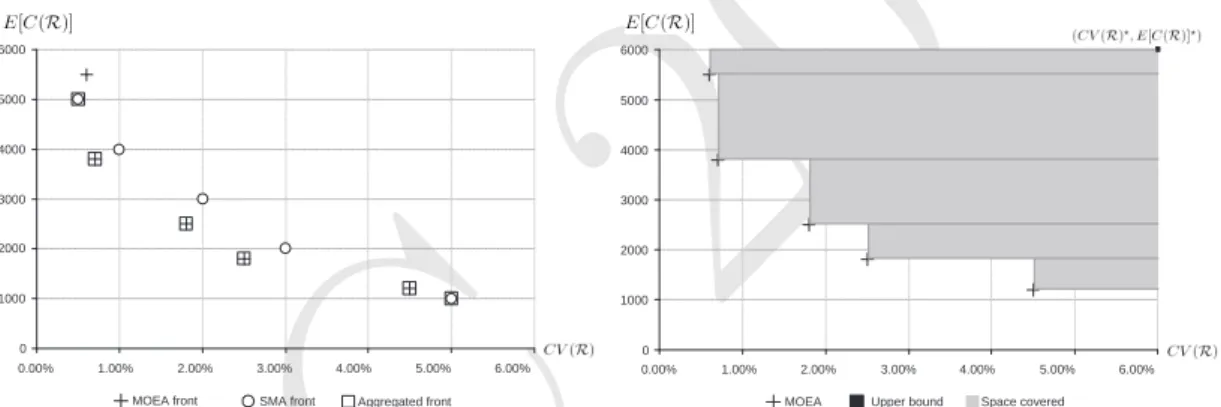
reports the fraction of solutions contributed by each algorithm to an aggregated front obtained by combining the solutions of both algorithms and selecting those that are nondominated. The latter reports the fraction of the nondominated solutions generated by each algorithm that are truly nondominated, that is, they appear in the aggregated front. Figure 2(a) illustrates these two metrics by means of an example. While the MOEA and SMA fronts are both comprised of 5 nondominated solutions, the aggregated front contains 6 solutions, four of them from MOEA and just two from SMA. Consequently, the absolute and relative quality are 0.66(= 4/6) and 0.80(= 4/5) for MOEA; and 0.33(= 2/6) and 0.40(= 2/5) for SMA.

The third metric known as the Size of the Space Covered (SSC) was proposed by Zitzler et al. [14]; it estimates the quality of the Pareto front by measuring the size of the space enclosed by the frontier and a reference point. In general, the larger the enclosed space, the better the approximation. As an example, Figure 2(b) shows the space enclosed by the MOEA front and the reference point (CV (R)?_{, E[C(R)]}?_{), defined by two upper bounds of the objective functions (4)}

and (3), respectively. The value of the SSC metric is given by the union of the dominated spaces (shown in gray) generated by each solution in the front. To compare MOEA against SMA, we calculate for each experiment the SSC metric for both methods and compare the approaches using the number of best solutions, that is, the number of instances in which the method has the best SSC metric, and the deviation relative to the best, given by εbest= (SSCbest−SSCmethod)/SSCbest.

0 1000 2000 3000 4000 5000 6000 0.00% 1.00% 2.00% 3.00% 4.00% 5.00% 6.00% Aggregated front MOEA front SMA front

(a) Relative and absolute quality: SMA, MOEA, and aggregated fronts

0 1000 2000 3000 4000 5000 6000 0.00% 1.00% 2.00% 3.00% 4.00% 5.00% 6.00% MOEA Upper bound Space covered

(b) Size of the space covered metric: MOEA front

Figure 2: Examples of performance metrics

4.3 Results

After fine tuning the set of parameters for both MOEA (P = 80, T = 2000, pc= 0.75, pm = 0.10,

and p_ls = 0.2) and SMA (P = 80, T = 1000, p_c = 0.5, p_m = 0.20, p_ls = 0.2, ∆ = 10), the two methods were tested on a set of 30 randomly generated instances. For every instance, 50 customers were randomly distributed over a 100 × 100 Euclidean space; each client v demands three different products (p = 1, 2, 3) following a Normal distribution N (µv,p, σv,p), where µv,prandomly falls within

[10, 100] and σv,p is set such that the coefficient of variation σv,p/µv,p is 0.3; the capacity of the

compartments was set meeting a tightness ratio (P_v∈V\{0}µv,p)/Qp = 15; and last, the maximum

distance per route was set as L = θ×max_v∈V\{0}d0,v, where θ is uniformly distributed between 3 and

4. A single run of each method was executed on every instance using two values of β (0.1 and 0.4) for the distance constraint (5). All the experiments were conducted using (1 − α) = 0.95 and γ = 0.05 as parameters for the Monte Carlo simulation model. Both SMA and MOEA were coded in Java

MIC

2009

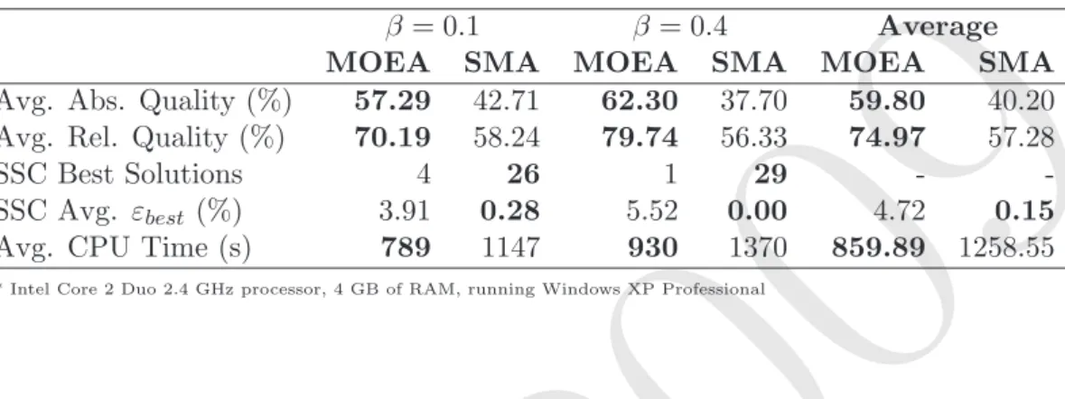
using Multiobjective Java Genetic Algorithms (MO-JGA), an object-oriented framework for the rapid development of multiobjective evolutionary algorithms [7]. The support for the generation of random numbers in the Monte Carlo simulation model is provided by the package Stochastic Simulation in Java (SSJ) [6].

Table 1: Computational experiments on a set of 30 randomly generated instances

β = 0.1 β = 0.4 Average

MOEA SMA MOEA SMA MOEA SMA

Avg. Abs. Quality (%) 57.29 42.71 62.30 37.70 59.80 40.20

Avg. Rel. Quality (%) 70.19 58.24 79.74 56.33 74.97 57.28

SSC Best Solutions 4 26 1 29 -

-SSC Avg. εbest (%) 3.91 0.28 5.52 0.00 4.72 0.15

Avg. CPU Time (s) 789 1147 930 1370 859.89 1258.55

* Intel Core 2 Duo 2.4 GHz processor, 4 GB of RAM, running Windows XP Professional

Table 1 reports the average values for the three performance metrics and the execution time over the 30 instances. In terms of quality, the results show that MOEA dominates SMA in both the absolute and relative measures. In terms of the absolute quality, MOEA provides on average 59.8% of the solutions of the aggregated front, while SMA provides only 40.2%. This gap is even more significant when the distance constraint is relaxed (higher value of β). On the experiments conducted with β = 0.1 the gap is 15.58% (= 57.29 − 42.71), while it reaches 24.60% (= 62.30 − 37.70) when

β = 0.4. A plausible explanation for this behavior is that larger values of β translate into larger

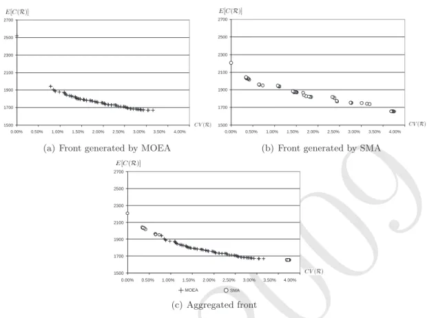
search spaces. Thus, there are more tradeoffs between the two objectives (i.e., routing alternatives) to be explored; a feature that is better exploited by the biobjective search of MOEA than the intensive single-objective search of SMA. In terms of relative quality, the results show that an important fraction of the solutions generated by both methods, nearly 75% for MOEA and 60% for SMA, turn to be nondominated in the aggregated front. The explanation of this result is well illustrated by the aggregated front plotted in Figure 3(c). Note that the solutions provided by the MOEA are densely spread along the central region of the front, while those provided by SMA are concentrated at the ends of the front. In other words, the two methods complement each other. While SMA is capable of finding good solutions for each single objective, MOEA is able to unveil a large set of tradeoffs between the two objectives. Although it is only illustrated for one instance, the behavior shown in Figure 3(c) is typical along the thirty instances comprised in the testbed.

Regarding the size of the space covered (SSC), the results show that SMA dominates MOEA. Even thought the fronts generated by SMA covered larger spaces in 92% (= 55/60) of the exper-iments, in terms of the deviation with respect to the best solution the difference between MOEA and SMA is only 4.57% (4.72 − 0.15), meaning that the fronts produced by both methods cover spaces of similar size. The better results of SMA can be explained by its ability to find extreme solutions. As shown in Figures 3(a) and 3(b), SMA is able to find a larger number of solutions with low coefficient of variation CV (R) than MOEA. These extreme solutions generate large dominated spaces that contribute significantly to the value of the SSC metric.

MIC

2009

1500 1700 1900 2100 2300 2500 2700 0.00% 0.50% 1.00% 1.50% 2.00% 2.50% 3.00% 3.50% 4.00%

(a) Front generated by MOEA

1500 1700 1900 2100 2300 2500 2700 0.00% 0.50% 1.00% 1.50% 2.00% 2.50% 3.00% 3.50% 4.00%

(b) Front generated by SMA

1500 1700 1900 2100 2300 2500 2700 0.00% 0.50% 1.00% 1.50% 2.00% 2.50% 3.00% 3.50% 4.00% MOEA SMA (c) Aggregated front

Figure 3: Approximated Pareto fronts for an instance with 50 customers and 3 products solved for β = 0.1

5

Concluding remarks and future research

This paper introduces the biobjective MC-VRPSD, the problem of designing collection routes to serve customers who have independent stochastic demands for different products that must be transported in independent vehicle compartments due to product mixing constraints. Due to the stochastic demands, the executed routes may have a different cost each time the solution is imple-mented. Thus, the objective is to select the set of routes that minimizes (i) the expected value of the total cost of the transportation plan and (ii) its coefficient of variation. To solve the biobjec-tive MC-VRPSD this paper proposes a multiobjecbiobjec-tive evolutionary algorithm (MOEA) based on a stochastic programming with recourse formulation. The MOEA couples NSGA-II with a local search procedure and bio-split, a novel evaluation and reparation strategy based on Monte Carlo simulation. To assess the performance of the MOEA, an alternative solution approach called SMA was implemented. SMA approximates the Pareto front by solving with a Memetic Algorithm the single-objective counterpart of the MC-VRPSD. SMA solves a sequence of problems minimizing the total expected cost, subject to different levels of the coefficient of variation. The two new methods were tested on a set of randomly generated instances with 50 clients and 3 products. The results show that the proposed MOEA is faster than SMA and produces approximate Pareto fronts of higher absolute and relative better quality. On the other hand, SMA is able to unveil nondomi-nated solutions at the ends of the Pareto front, unveiling a larger dominondomi-nated space according to the SSC metric. Research currently underway includes the development of new diversification and local search mechanisms that allow the MOEA to explore extreme solutions (thus covering larger

domi-MIC

2009

nated spaces); and the implementation of new simulation components and acceleration techniques that could reduce the computational burden on larger instances.

References

[1] K. Deb, A. Pratap, A. Sameer, and T. Meyarivan. A fast and elitist multiobjective genetic algorithm: NSGA-II. IEEE Transactions on Evolutionary Computation, 6(2):182–197, 2002.

[2] M. Gendreau, G. Laporte, and R. S´eguin. Stochastic vehicle routing. European Journal of

Operational Research, 88(1):3–12, 1996.

[3] Y. Y. Haimes, L. Lasdon, and D. A. Wismer. On a bicriterion formulation of the problems of integrated system identification and system optimization. IEEE Transactions on Systems,

Man, and Cybernetics, SMC-1(3):296–297, 1971.

[4] A. Jaszkiewicz. Evaluation of multiple objective metaheuristics. In X. Gandibleux, M. Sevaux, K. S¨orensen, and V. T’kindt, editors, Metaheuristics for Multiobjective Optimisation, volume 535 of Lecture Notes in Economics and Mathematical Systems. Springer, Berlin, 2004.

[5] A. M. Law and W. D. Kelton. Simulation Modeling and Analysis. McGraw-Hill, 2000.

[6] P. L’Ecuyer, L. Meliani, and J. Vaucher. SSJ: A framework for stochastic simulation in java. In E. Y¨ucesan, C. H. Chen, J. L. Snowdon, and J. M. Charnes, editors, Proceedings of the 2002

Winter Simulation Conference, pages 234–242. IEEE Press, 2002.

[7] A. L. Medaglia, E. Guti´errez, and Villegas J. G. Solving facility location problems using a tool for rapid develpment of Multi-Objective Evolutionary Algorithms (MOEAS). In Jean-Phillipe Rennard, editor, Handbook of Research on Nature Inspired Computing for Economics

and Management. Idea Publishing Group, 2006.

[8] J. E. Mendoza, B. Castanier, C. Gu´eret, A. L. Medaglia, and N. Velasco. A memetic algorithm for the multi-compartment vehicle routing problem with stochastic demands. Working paper. http://hdl.handle.net/1992/1106, 2009.

[9] J. E. Mendoza, A. L. Medaglia, and N. Velasco. An evolutionary-based decision support sytem for vehicle routing: the case of a public utility. Decision Support Systems, 46(3):730–742, 2009.

[10] S. M. Mulvey, R. J. Vanderbei, and S. A. Zenios. Robust optimization of large-scale systems.

Operation Research, 43(2):264–281, 1995.

[11] F. B. Pereira, J. Tavares, P. Machado, and E. Costa. GVR: a new genetic representation for the vehicle routing problem. In Proceedings of AICS 2002 - 13th Irish Conference on Artificial

Intelligence and Cognitive Science, 2002.

[12] C. Prins. A simple and effective evolutionary algorithm for the vehicle routing problem.

Com-puters and Operations Research, 31(12):1985–2002, 2004.

[13] W. H. Yang, K. Mathur, and R. Ballou. Stochastic vehicle routing with restocking.

Trans-portation Science, 34(1):99–112, 2000.

[14] E. Zitzler and L. Thiele. Multiobjective optimization using evolutionary algorithms - a compar-ative case study. In Parallel Problem Solving from Nature (PPSN) V, pages 292–301. Springer, 1998.