Université de Montréal
Learning visual representations with neural networks
for video captioning and image generation
par
Li Yao
Département d’ informatique et de recherche opérationnelle Faculté des arts et des sciences
Thèse présentée à la Faculté des études supérieures en vue de l’obtention du grade de
Philosophiæ Doctor (Ph.D.) en informatiques
décembre 2017
c
RÉSUMÉ
La recherche sur les réseaux de neurones a permis de réaliser de larges progrès durant la dernière décennie. Non seulement les réseaux de neurones ont été appliqués avec succès pour résoudre des problèmes de plus en plus complexes; mais ils sont aussi devenus l’approche dominante dans les domaines où ils ont été testés tels que la compréhension du langage, les agents jouant à des jeux de manière automatique ou encore la vision par ordinateur, grâce à leurs capacités calculatoires et leurs efficacités statistiques.
La présente thèse étudie les réseaux de neurones appliqués à des problèmes en vision par ordinateur, où les représentations sémantiques abstraites jouent un rôle fondamental. Nous démontrerons, à la fois par la théorie et par l’expérimentation, la capacité des réseaux de neurones à apprendre de telles représentations à partir de données, avec ou sans supervision. Le contenu de la thèse est divisé en deux parties. La première partie étudie les réseaux de neurones appliqués à la description de vidéo en langage naturel, nécessitant l’apprentissage de représentation visuelle. Le premier modèle proposé permet d’avoir une attention dynamique sur les différentes trames de la vidéo lors de la génération de la description textuelle pour de courtes vidéos. Ce modèle est ensuite amélioré par l’introduction d’une opération de convolution récurrente. Par la suite, la dernière section de cette partie identifie un problème fondamental dans la description de vidéo en langage naturel et propose un nouveau type de métrique d’évaluation qui peut être utilisé empiriquement comme un oracle afin d’analyser les performances de modèles concernant cette tâche.
La deuxième partie se concentre sur l’apprentissage non-supervisé et étudie une famille de modèles capables de générer des images. En particulier, l’accent est mis sur les “Neural Autoregressive Density Estimators (NADEs), une famille de modèles probabilistes pour les images naturelles. Ce travail met tout d’abord en évidence une connection entre les modèles NADEs et les réseaux stochastiques génératifs (GSN). De plus, une amélioration des modèles NADEs standards est proposée. Dénommés NADEs itératifs, cette amélioration introduit plusieurs itérations lors de l’inférence du modèle NADEs tout en préservant son nombre de paramètres.
Débutant par une revue chronologique, ce travail se termine par un résumé des récents développements en lien avec les contributions présentées dans les deux parties principales,
concernant les problèmes d’apprentissage de représentation sémantiques pour les images et les vidéos. De prometteuses directions de recherche sont envisagées.
Mot clés: réseaux de neurones, apprentissage de représentations, description naturelle
ABSTRACT
The past decade has been marked as a golden era of neural network research. Not only have neural networks been successfully applied to solve more and more challenging real-world problems, but also they have become the dominant approach in many of the places where they have been tested. These places include, for instance, language understanding, game playing, and computer vision, thanks to neural networks’ superiority in computational efficiency and statistical capacity.
This thesis applies neural networks to problems in computer vision where high-level and semantically meaningful representations play a fundamental role. It demonstrates both in theory and in experiment the ability to learn such representations from data with and without supervision.
The main content of the thesis is divided into two parts. The first part studies neural networks in the context of learning visual representations for the task of video captioning. Models are developed to dynamically focus on different frames while generating a natural language description of a short video. Such a model is further improved by recurrent convolu-tional operations. The end of this part identifies fundamental challenges in video captioning and proposes a new type of evaluation metric that may be used experimentally as an oracle to benchmark performance.
The second part studies the family of models that generate images. While the first part is supervised, this part is unsupervised. The focus of it is the popular family of Neural Autoregressive Density Estimators (NADEs), a tractable probabilistic model for natural images. This work first makes a connection between NADEs and Generative Stochastic Networks (GSNs). The standard NADE is improved by introducing multiple iterations in its inference without increasing the number of parameters, which is dubbed iterative NADE.
With a historical view at the beginning, this work ends with a summary of recent devel-opment for work discussed in the first two parts around the central topic of learning visual representations for images and videos. A bright future is envisioned at the end.
keywords: neural networks, representation learning, video captioning, unsupervised
CONTENTS
Résumé. . . . i Abstract. . . . iii List of figures. . . . xi List of tables. . . . xv Acknowledgement. . . . xviiChapter 1. Machine learning. . . . 1
1.1. Machine learning and its relation with other subjects. . . 1
1.2. Formalizing learning. . . 2
1.2.1. Basic idea of Bayesian learning. . . 3
1.2.2. Frequentist learning . . . 3
1.2.3. Parametric and non-parametric learning. . . 5
1.3. Learning to generalize. . . 6
1.3.1. Generalization in supervised learning. . . 6
1.3.2. Generalization in unsupervised learning. . . 7
1.3.3. Formalizing the generalization error. . . 7
1.3.4. Model selection. . . 7
1.3.4.1. Bayesian model averaging . . . 8
1.3.4.2. Cross-validation. . . 8
1.3.4.3. Bagging and boosting. . . 8
1.4. The curse of dimensionality and its implication. . . 9
Chapter 2. Representation learning. . . . 11
2.1. Challenging problems in the AI-set. . . 11
2.2. Learning hierarchical and distributed representations. . . 12
2.4. Recurrent neural networks. . . 15
2.5. Auto-encoders. . . 16
2.6. Graphical models based neural networks. . . 17
2.6.1. Directed graphical models. . . 18
2.6.2. Variational autoencoders . . . 20
2.6.3. Markov random fields. . . 20
2.7. Computational techniques. . . 23
2.7.1. Optimization. . . 23
2.7.2. Sampling in graphical models. . . 26
2.7.2.1. Markov chain Monte Carlo. . . 26
Chapter 3. Learning visual representations. . . . 29
3.1. The computer vision challenge. . . 29
3.2. visual representations. . . 29
3.3. Traditional approaches. . . 31
3.3.1. Image descriptors and encoding. . . 31
3.3.2. Video descriptors and encoding. . . 33
3.4. Learning-based approaches. . . 33
3.4.1. Supervised learning of visual representation. . . 33
3.4.2. Unsupervised learning of visual representation. . . 34
Chapter 4. Prologue to first article. . . . 37
4.1. Article Detail. . . 37
4.2. Context. . . 37
4.3. Contributions. . . 38
Chapter 5. Describing Videos by Exploiting Temporal Structure. . . . . 39
5.1. Introduction. . . 39
5.2. Video Description Generation Using an Encoder–Decoder Framework. . . . 41
5.2.1. Encoder-Decoder Framework. . . 41
5.2.2. Encoder: Convolutional Neural Network. . . 42
5.3. Exploiting Temporal Structure in Video Description Generation. . . 44
5.3.1. Exploiting Local Structure: A Spatio-Temporal Convolutional Neural Net. . . 44
5.3.2. Exploiting Global Structure: A Temporal Attention Mechanism. . . 46
5.4. Related Work. . . 47 5.5. Experiments. . . 48 5.5.1. Datasets. . . 48 5.5.1.1. Youtube2Text. . . 48 5.5.1.2. DVS. . . 49 5.5.2. Description Preprocessing. . . 49 5.5.3. Video Preprocessing. . . 49 5.5.4. Experimental Setup. . . 50 5.5.4.1. Models. . . 50 5.5.4.2. Training. . . 51 5.5.4.3. Evaluation. . . 51 5.5.5. Quantitative Analysis. . . 51 5.5.6. Qualitative Analysis. . . 52 5.6. Conclusion. . . 53 Acknowledgments. . . 53
Chapter 6. Prologue to second article. . . . 55
6.1. Article Detail. . . 55
6.2. Context. . . 55
6.3. Contributions. . . 56
Chapter 7. Oracle Performance for Visual Captioning. . . . 57
7.1. Introduction. . . 57
7.2. Related work. . . 58
7.2.1. Visual captioning. . . 58
7.2.2. Capturing higher-level visual concept. . . 59
7.3. Oracle Model. . . 59
7.3.2. Atoms Construction. . . 61
7.4. Contributing factors of the oracle. . . 61
7.5. Experiments. . . 62
7.5.1. Atom extraction. . . 62
7.5.2. Training. . . 64
7.5.3. Interpretation. . . 64
7.5.3.1. comparing oracle performance with existing models. . . 64
7.5.3.2. quantify the diminishing return. . . 64
7.5.3.3. atom accuracy versus atom quantity. . . 66
7.5.3.4. intrinsic difficulties of particular datasets. . . 66
7.6. Discussion. . . 67
Acknowledgments. . . 68
Chapter 8. Prologue to third article. . . . 69
8.1. Article Detail. . . 69
8.2. Context. . . 69
8.3. Contributions. . . 70
Chapter 9. Delving Deeper into Convolutional Networks for Learning Video Representations. . . . 71
9.1. Introduction. . . 71
9.2. GRU: Gated Recurrent Unit Networks. . . 73
9.3. Delving Deeper into Convolutional Neural Networks. . . 73
9.3.1. GRU-RCN. . . 74 9.3.2. Stacked GRU-RCN: . . . 75 9.4. Related Work. . . 76 9.5. Experimentation. . . 76 9.5.1. Action Recognition. . . 77 9.5.1.1. Model Architecture. . . 77
9.5.1.2. Model Training and Evaluation. . . 78
9.5.1.3. Results. . . 78
9.5.2.1. Model Specifications. . . 80
9.5.2.2. Training. . . 80
9.5.2.3. Results. . . 81
9.6. Conclusion. . . 82
Acknowledgments. . . 82
Chapter 10. Prologue to fourth article. . . . 83
10.1. Article Detail. . . 83
10.2. Context. . . 83
10.3. Contributions. . . 84
Chapter 11. On the Equivalence Between Deep NADE and Generative Stochastic Network. . . . 85
11.1. Introduction. . . 85
11.2. Deep NADE and Order-Agnostic Training. . . 86
11.2.1. NADE. . . 87
11.2.2. Deep NADE. . . 87
11.3. Generative Stochastic Networks. . . 88
11.4. Equivalence between deep NADE and GSN. . . 90
11.4.1. Alternative Sampling Method for NADE. . . 91
11.4.2. The GSN Chain Averages an Ensemble of Density Estimators. . . 92
11.5. Annealed GSN Sampling. . . 92
11.6. Experiments. . . 94
11.6.1. Settings: Dataset and Model . . . 94
11.6.2. Qualitative Analysis. . . 95
11.6.3. Quantitative Results. . . 95
11.7. Conclusions. . . 97
Acknowledgments. . . 98
Chapter 12. Prologue to fifth article. . . . 99
12.2. Context. . . 99
12.3. Contributions. . . 100
Chapter 13. Iterative Neural Autoregressive Distribution Estimator (NADE-k). . . . 101
13.1. Introduction. . . 101
13.2. Proposed Method: NADE-k. . . 102
13.2.1. Related Methods and Approaches. . . 104
13.3. Experiments. . . 106
13.3.1. MNIST. . . 106
13.3.1.1. Qualitative Analysis. . . 109
13.3.1.2. Variability over Orderings. . . 109
13.3.2. Caltech-101 silhouettes. . . 109
13.4. Conclusions and Discussion. . . 110
Acknowledgements. . . 112
Chapter 14. Recent development in learning visual representations. . . 113
14.1. Learning image representations. . . 113
14.2. Learning video representations. . . 114
Chapter 15. Conclusion. . . . 117
LIST OF FIGURES
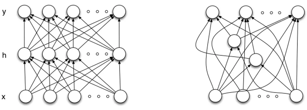
2.1 Left: A feed-forward neural network with one input layer, one hidden layer,
and one output layer. Right: A feed-forward neural network in a general form
whose organization is not according to layers.. . . 14
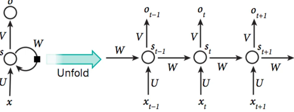
2.2 Left: An RNN with one recurrent layer, one input layer and one output layer.
Right: An RNN unfolds itself over time steps to form a feed-forward model
with shared hidden layers The figure is credited by LeCun et al. (2015). . . 15
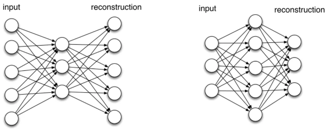
2.3 Left: A standard auto-encoder must have an information bottleneck in the
hidden layer to avoid learning the trivial identity reconstruction function. Right: A regularized auto-encoder that can have an over-complete hidden layer, such as denoising auto-encoders, and contractive auto-encoders since it
cannot learn the identity function.. . . 16
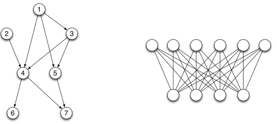
2.4 Left: An example of directed graphical models. Edges are directed. The
number in the nodes indicates a topological order. Right: The Restricted Boltzmann machine as an example of undirected graphical models. Edges are
undirected.. . . 18
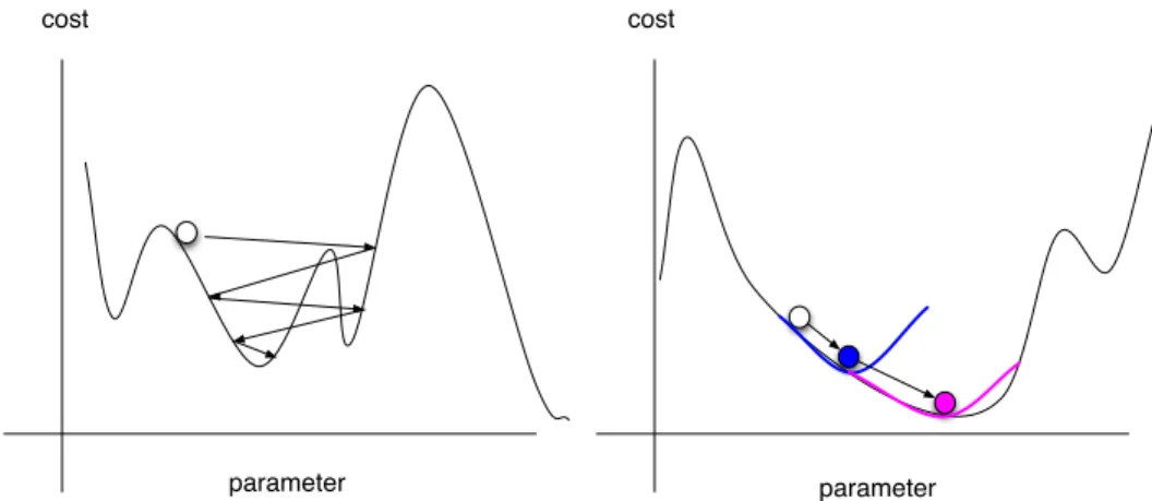
2.5 Left: SGD uses noisy gradient to reach global minima.Right: Second order
optimization methods use a local quadratic approximation and move to the
minimum of a quadratic curve at each step.. . . 24
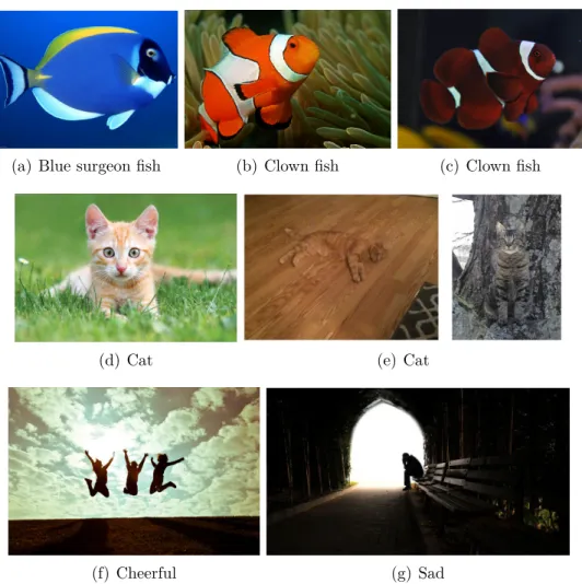
3.1 A good representation is invariant to the physical interactions and environmental changes such as (a) – (e). A good representation may not be easily defined
with handwritten rules such as (f) and (g).. . . 30
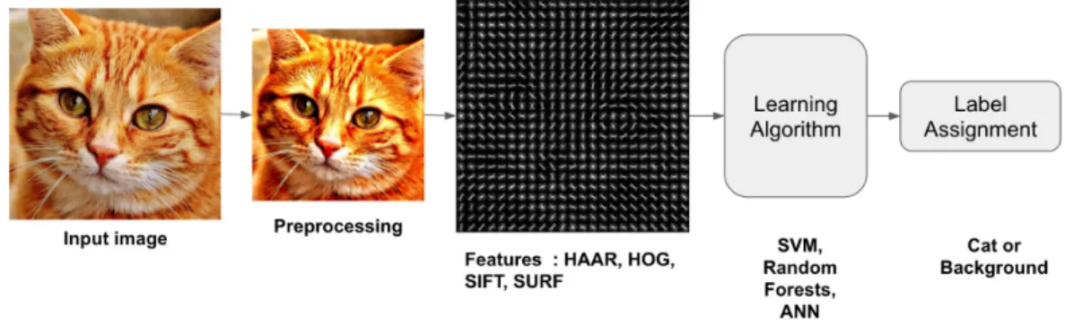
3.2 Credit: http://www.learnopencv.com/. Classical computer vision approach may be separated into several stages each of which has its particular set of
algorithms.. . . 31
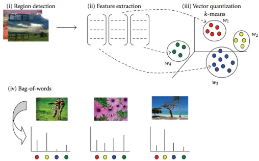
3.3 Credit: (Tsai, 2012). Bag of visual words representation for images. Region-based descriptors are first clustered by k-means in (iii), followed by a histogram
where each bin is a cluster, the size of the bin being the number of regional
descriptors that fall within that cluster.. . . 32
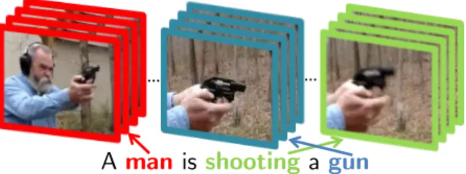
5.1 High-level visualization of our approach to video description generation. We incorporate models of both the local temporal dynamic (i.e. within blocks of a few frames) of videos, as well as their global temporal structure. The local structure is modeled using the temporal feature maps of a 3-D CNN, while a temporal attention mechanism is used to combine information across the entire video. For each generated word, the model can focus on different temporal regions in the video. For simplicity, we highlight only the region
having the maximum attention above.. . . 40
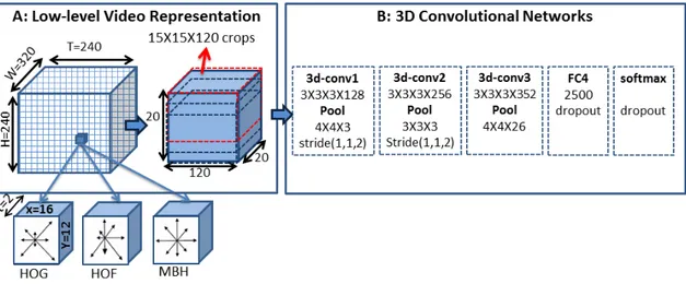
5.2 Illustration of the spatio-temporal convolutional neural network (3-D CNN). This
network is trained for activity recognition. Then, only the convolutional layers are
involved when generating video descriptions. . . 45
5.3 Illustration of the proposed temporal attention mechanism in the LSTM
decoder. . . 46
5.4 Four sample videos and their corresponding generated and ground-truth descriptions from Youtube2Text (Left Column) and DVS (Right Column). The bar plot under each frame corresponds to the attention weight αt
i for the
frame when the corresponding word (color-coded) was generated. From the top left panel, we can see that when the word “road” is about to be generated, the model focuses highly on the third frame where the road is clearly visible. Similarly, on the bottom left panel, we can see that the model attends to the second frame when it was about to generate the word “Someone”. The bottom
row includes alternate descriptions generated by the other model variations. 52
7.1 Given ground truth captions, three categories of visual atoms (entity, action and attribute) are automatically extracted using NLP Parser. “NA” denotes
the empty atom set.. . . 63
7.2 Learned oracle on COCO (left), YouTube2Text (middle) and LSMDC (right). The number of atoms a(k) is varied on x-axis and oracles are computed on
y-axis on testsets. The first row shows the oracles on BLEU and METEOR with 3k atoms, k from each of the three categories. The second row shows the oracles when k atoms are selected individually for each category. CIDEr is used for COCO and YouTube2Text as each test example is associated
with multiple ground truth captions, argued in (Vedantam et al., 2014). For
LSMDC, METEOR is used, as argued by Rohrbach et al. (2015).. . . 65
7.3 Learned oracles with different atom precision (r in red) and atom quantity (x-axis) on COCO (left) and LSMDC (right). The number of atoms ˆar(k) is varied on x-axis and oracles are computed on y-axis on testsets. CIDEr is used for COCO and METEOR for LSMDC. It shows one could increase the score by either improving P (a(k)|v) with a fixed k or increase k. It also shows
the maximal error bearable for different score.. . . 67
9.1 Visualization of convolutional maps on successive frames in video. As we go up in the CNN hierarchy, we observe that the convolutional maps are more
stable over time, and thus discard variation over short temporal windows.. . . 72
9.2 High-level visualization of our model. Our approach leverages convolutional maps from different layers of a pretrained-convnet. Each map is given as input to a convolutional GRU-RNN (hence GRU-RCN) at different time-step. Bottom-up connections may be optionally added between RCN layers to form
Stack-GRU-RCN. . . 74
11.1 Independent samples generated by the ancestral sampling procedure from the
deep NADE. . . 93
11.2 The consecutive samples from the two independent GSN sampling chains without any annealing strategy. Both chains started from uniformly random configurations. Note the few spurious samples which can be avoided with the
annealing strategy (see Figure 11.3). . . 94
11.3 Samples generated by the annealed GSN sampling procedure for the same deep NADE model. Visually the quality is comparable to the ancestral samples, and mixing is very fast. This is obtained with pmax= 0.9, pmin = 0.1,
α = 0.7 and T = 20. . . . 96
11.4 The annealed GSN sampling procedure is compared against NADE ancestral sampling, trading off the computational cost (computational wrt to ancestral sampling on x-axis) against log-likelihood of the generated samples (y-axis). The computational cost discards the effect of the Markov chain autocorrelation by estimating the effective number of samples and increasing
13.1 The choice of a structure for NADE-k is very flexible. The dark filled halves indicate that a part of the input is observed and fixed to the observed values during the iterations. Left: Basic structure corresponding to Equations (13.2.6–13.2.7) with n = 2 and k = 2. Middle: Depth added as in NADE by Uria et al. (2014) with n = 3 and k = 2. Right: Depth added as in Multi-Prediction Deep Boltzmann Machine by Goodfellow et al. (2013) with
n = 2 and k = 3. The first two structures are used in the experiments. . . . 103
13.2 The inner working mechanism of NADE-k. The left most column shows the data vectors x, the second column shows their masked version and the
subsequent columns show the reconstructions vh0i. . . vh10i(See Eq. (13.2.7)). 104
13.3 NADE-k with k steps of variational inference helps to reduce the training cost (a) and to generalize better (b). NADE-mask performs better than NADE-1
without masks both in training and test.. . . 108
13.4 (a) The generalization performance of different NADE-k models trained with different k. (b) The generalization performance of NADE-5 2h, trained with
k=5, but with various k in test time.. . . 108
13.5 Samples generated from NADE-k trained on (a) MNIST and (b) Caltech-101
Silhouettes.. . . 110
13.6 Filters learned from NADE-5 2HL. (a) A random subset of the encodering
LIST OF TABLES
5. I Performance of different variants of the model on the Youtube2Text. . . 50
5. II Performance of different variants of the model on the DVS. . . 50
7. I Human evaluation of proportion of atoms that are voted as visual. It is clear that extracted atoms from three categories contain dominant amount of visual elements, hence verifying the procedure described in Section 7.3.2. Another observation is that entities and actions tend to be more visual than attributes
according to human perception.. . . 63
7. II
Measure semantic capacity of current state-of-the-art models. One could easily map the reported metric to the number of visual atoms captured. This establishes an equivalence between a model, the proposed oracle and a model’s semantic capacity. (“ENT” for entities. “ACT” for actions. “ATT” for attributes. “ALL” for all three categories combined. “B1” for BLEU-1, “B4” for BLEU-4. “M” for METEOR. “C” for CIDEr. Note that the CIDEr
is between 0 and 10. The learned oracle is denoted in bold.. . . 66
9. I Classification accuracy of different variants of the model on the UCF101 split 1. We report the performance of previous works that learn representation
using only RGB information only.. . . 79
9. II Performance of different variants of the model on YouTube2Text for video captioning. Representations obtained with the proposed RCN architecture combined with decoders fromYao et al.(2015a) offer a significant performance
boost, reaching the performance of the other state-of-the-art models.. . . 81
11. I Log-probability of 1000 samples when anealing is not used. To collect samples, 100 parallel chains are run and 10 samples are taken from each chain and combined together. The noise level is fixed at a particular level during the sampling. We also report the best log-probability of samples generated with
13. I Results obtained on MNIST using various models and number of hidden layers (1HL or 2HL). “Ords” is short for “orderings”. These are the average log-probabilities of the test set. EoNADE refers to the ensemble probability (See Eq. (13.2.9)). From here on, in all figures and tables we use “HL” to
denote the number of hidden layers and “h” for the number of hidden units. 107
13. II The variance of log p(x | o) over orderings o and over test samples x. . . . 109
13. IIIAverage log-probabilities of test samples of Caltech-101 Silhouettes. (?) The results are from Cho et al. (2013). The terms in the parenthesis indicate the number of hidden units, the total number of parameters (M for million), and the L2 regularization coefficient. NADE-mask 670h achieves the best
ACKNOWLEDGEMENT
First of all, I would like to thank Prof. Yoshua Bengio for being a rock-star teacher and supervisor. I clearly remember my early days of graduate school when we sat down together debugging codes. My favorite quote from him is “Being a good researcher is like being a detective who does not overlook any suspicion in the code and in the experiments”. I remember the day when we got our first successful experiment for the NIPS paper in 2013 and he was so excited and we did Hi-Five three times. What I have learned from Prof. Bengio is that a scientist lives and breathes science, which I still find it hard to follow from time to time. All my work on unsupervised learning in this thesis were done with Prof. Bengio. He taught me to see models from a probabilistic point of view, be organized, patient and persevere in debugging and analyzing experiments.
I would also like to thank many people who have taught me so much in the past 5 years. Prof. Aaron Courville have worked with me closely on video projects and supported me through those sunny and rainy days. Prof. Kyunghyun Cho, who has been my co-author for almost all of my publications taught me the importance of scientific writing and his brilliance has been my inspiration for all these years. Dr. Nicolas Ballas spent most of his post-doc doing research with me, with whom I had my most productive period. In addition, I would like to thank people who have helped me with my research in various ways: Prof. Hugo Larochelle from Google, Dr. Razvan Pascanu, Dr. Guillaume Desjardins from DeepMind, Dr. John Smith from IBM Research, Dr. Orhan Firat from Google, and many other staff members, fellow students and visitors in the MILA lab.
Lastly, I would like to thank my parents who support me during my academic career all these years since I left China for Finland almost 8 years ago. They encourage me to explore my potential and pursue my dream. I would also like to thank my girlfriend Marie whom I met in Montréal and who has the courage to follow me to the strange land of San Francisco to start a new life with me.
Chapter
1
MACHINE LEARNING
Machine learning, a subject grown out of the intersection of statistics, psychology, neu-roscience and artificial intelligence, has prospered during the past few decades. The first chapter looks at its historical development, reviews its core theory, exemplifies some of its most popular models, and exposes the computational challenge ahead.
1.1. Machine learning and its relation with other subjects
Machine learning studies algorithms that learn patterns from data. Under the assumption that there exists an unknown data generating process, the purpose of learning is to uncover some aspects of it based on data samples it generates. Since the same data may be generated by any process, learning is only possible when some assumptions on the data generating process is made. This assumption is called the inductive bias that represents a hypothesis space where a learning algorithm searches to find the best possible hypothesis, or model, that explains the data. The need for establishing a hypothesis space is best demonstrated by the famous no-free-lunch theorem (Wolpert,1996). The theorem shows that there is no universal best model. The reason is that one set of assumptions that works well in one domain may work poorly in another. This theorem diminishes the hope of finding a general-purpose learning algorithm that is able to solve all problems without any tuning. It motivates the necessity of injecting assumptions or prior knowledge of human experts into the effort of making an effective learning algorithm. In other words, learning requires prior knowledge.
Historically, machine learning grew out of the subject of artificial intelligence. In artificial intelligence, the goal is to construct an intelligent agent that possesses some human-like skills. To achieve that ambitious goal, an intelligent agent must be able to understand the surroundings and to take actions. This requires the skills of knowledge representation, reasoning, planning, and robotic control to be practically realizable. So far this goal remains elusive. Machine learning takes a step back and focuses on knowledge representation and reasoning. This was unified under the theory of probability by Pearl (1988). Knowledge is built into a probabilistic model and decision making is formalized by probabilistic inference.
Another line of development for machine learning grew out of the goal of understanding the working mechanism of the human brain in psychology and computational neuroscience. One of the earliest development in this direction is the McCulloch-Pitts Neuron (McCulloch and Pitts, 1943a) where a biological neuron is mathematically simplified in a spectacular fashion and still proved to be useful in solving some difficult tasks. This type of simple neuron, when organized in a hierarchy, has claimed many of the state-of-the-art results on machine learning benchmarks to date. Computational neuroscience is exemplified by biological inspired models such as Hierarchical Temporal Memory (HTM) (Hawkins and Blakeslee, 2004) and Hierarchical Model and X (HMAX) (Riesenhuber and Poggio, 1999). HTM consists of artificial neurons that are more biologically plausible and has been proved to be useful at modelling time series. HMAX has been widely accepted as the standard model of visual cortex. The recent study of Bengio et al.(2015) shed some light on the connection between synaptic weight updates and a particular form of variational EM algorithm.
1.2. Formalizing learning
Following tradition, learning is divided into three categories. Supervised learning, un-supervised learning and reinforcement learning. Supervised and unun-supervised learning are introduced below.
Supervised learning, such as classification and regression, focuses on the prediction of a target ~y given an observation ~x where ( ~xi, ~yi) ∼ P (~x, ~y). P (~x, ~y) is an unknown data generating distribution. In regression, ~y represents either a real-value scalar or a vector.
In classification, ~y usually represents a discrete code indicating which class ~x belongs to.
Predicting ~y given ~x is usually done by estimating P (~y|~x) using training pairs ( ~xi, ~yi). Unsupervised learning is more diversified. The majority of problems in this category can be considered as a problem of density estimation: given observations ~x ∼ P (~x), estimate
implicitly or explicitly the density P (~x).
There are two views of learning: Bayesian and frequentist. The two views differ in the way the concept probability is treated. Bayesian learning insists on using probability as a way to measure the degree of belief. On the other hand, frequentist learning treats probability as the frequency of occurrence for certain events . This yields different treatment of parameters specifying underlying probabilistic models. In Bayesian learning, there exists a probability distribution on the parameters. As training data are seen, the degree of belief, or the probability distribution, on model parameters shall be updated. On the other hand, frequentist learning assumes an unknown single value of a parameter. As training data are seen, a point estimation of a parameter is obtained by performing optimization with respect to some criterion. The difference between these two learning paradigms is illustrated below in terms of density estimation.
1.2.1. Basic idea of Bayesian learning
Although not directly used in the scope of this thesis, the important idea of Bayesian learning is briefly outlined below.
Given a training set D, the fully-fledged Bayesian models P (~x) as a marginalization over
all possible parameters θ.
P (~x|D) =
Z θ
P (~x|θ)P (θ|D)dθ (1.2.1)
where the posterior over the parameter θ is defined as
P (θ|D) = P (D|θ)P (θ)
P (D) (1.2.2)
One has to specify the parameterizations of both the prior P (θ) and the likelihood P (D|θ) in order to compute the posterior. When the marginalization in (1.2.1) is analytically in-tractable, one could fall back to the maximum a posteriori (MAP) estimation
θ?MAP= arg max θ
P (D|θ)P (θ) (1.2.3)
In MAP, P (~x|D) is approximated by
P (~x|D) ≈ P (~x|θ?MAP) (1.2.4)
(1.2.4) is a good approximation when the posterior over θ is unimodal and θ?
MAPis the mode.
As more data arrive, MAP in (1.2.4) and Bayesian prediction in (1.2.1) become closer, as MAP’s competing hypotheses become less likely. As is usually the case, performing numerical optimization is relatively easier than estimating the integral.
1.2.2. Frequentist learning
Frequentist learning focuses on the point estimation of the model parameters. One of the most popular frameworks is maximum likelihood estimation (MLE).
θMLE? = arg max θ
P (D|θ) (1.2.5)
MLE can be justified from various perspectives. MLE is closely related to the well-known Kullback-Leibler (KL) divergence that measures the discrepancy between two probability distributions. The KL divergence between the unknown data generating distribution P (~x)
and the model Pθ(~x) is defined as
KL(P (~x)||Pθ(~x)) = Z x P (~x) log P (~x) Pθ(~x) d~x (1.2.6) = Z x P (~x) log P (~x) − Z x P (~x) log Pθ(~x) (1.2.7)
where the second term on the right is called cross-entropy between P (~x) and Pθ(~x).The first term does not depend on θ. Using N training examples from D, The empirical minimization of the KL is written as ˆ θ?KL= arg min θ 1 N N X i=1 log P ( ~xi) Pθ( ~xi) (1.2.8)
where ~xi ∼ P (~xi). Under the assumption that the examples in D are independently identi-cally distributed (i.i.d.), the empirical risk minimization of log-likelihood can be written as follows:
ˆ
θ?MLE= arg max θ log( N Y i Pθ(~xi)) (1.2.9) = arg max θ N X i log Pθ(~xi) = arg max θ 1 N X i logPθ( ~xi) P ( ~xi) = arg min θ 1 N X i log P ( ~xi) Pθ( ~xi) = ˆθKL?
Thus maximizing the log-likelihood under the i.i.d. assumption is equivalent to minimizing the KL divergence between the model distribution and the true unknown distribution.
MLE suffers from overfitting (detailed in section 1.3) when training data is scarce or the model Pθ(~xi) is too complex. For instance, consider a dataset that only contains a few coin flips that are all heads. θ denotes the probability of a coin flip being heads. MLE results in θ = 1 since only heads are observed. This estimated value is highly unlikely and overconfident. With large datasets, this kind of overfitting is still possible when a model with a large number of parameters is used. Therefore in practice, it is common to use a regularized version of MLE
ˆ
θMLE? reg = arg max θ
[log P (D|θ) + λφ(θ)] (1.2.10)
where a regularization term φ(θ) penalizes the model complexity and λ weighs the penaliza-tion. There exists a connection between ˆθ?
MLEreg and θ
?
MAP in (1.2.3). θMAP? = arg max
θ
P (D|θ)P (θ) = arg max
θ
[log P (D|θ) + log P (θ)] (1.2.11)
Therefore, θ?
MAP is equivalent to ˆθ?MLEreg and the regularization term in ˆθ
?
MLEreg is interpreted
as the log of the prior P (θ).
As an estimator, the unbiasedness of MLE varies from case to case, for example, in estimating the mean µ and the standard deviation σ in a univariate Gaussian distribution
N (µ, σ), ˆµMLE = N1 Pnxiis unbiased but ˆσMLE2 = 1
N P
n(xi− ˆµMLE)2is biased. MLE has some
desirable properties as a default estimator in learning. Asymptotically, MLE is consistent, meaning Pθ(x) → P (x) as N → ∞. It is also asymptotically optimal or efficient in that it has the lowest variance among all the estimators. However MLE only provides a point estimation. Compared with Bayesian learning, it does not give any measure of uncertainty in the guess. Furthermore, MLE computation may also be expensive with complicated probabilistic models, which is usually the case in machine learning with high dimensional data. Other point estimators exist in machine learning. More tractable alternatives have been proposed such as Pseudo likelihood (Besag, 1975), ratio matching (Hyvärinen, 2007), generalized score matching (Lyu,2009), and minimum probability flow (Sohl-Dickstein et al.,
2009) and moment maching (Li et al., 2015).
1.2.3. Parametric and non-parametric learning
Orthogonal to the categorization of learning into supervised and unsupervised, an alter-native view is to differentiate learning algorithms between parametric and non-parametric. In parametric learning, the parameter has a fixed size that is independent of number of training examples N . Making predictions does not involve any explicit use of the historical data any more since P (~x|θ) is fully realizable by a function with the learned parameter θ.
One could argue that assuming any particular parameterization of P (~x|θ) raises questions
on the reliability of the assumption. This is indeed one shortcoming of parametric learning. Conversely, in non-parametric learning, P (~x) does not have a prefixed number of
pa-rameters and may grow automatically with more data. Indeed, most iconic non-parametric models such as K nearest neighbor classifiers and Parzen density estimators directly memo-rize the entire historical data. In particular, Parzen density estimator defines the probability density p(~x) = 1 N N X n=1 1 2πh2 exp(− ||~x − ~xn||2 2h2 ) (1.2.12)
at a particular point ~x as a linear combination of Gaussians that are centered at each training
example ~xi. Similarly, one can define a Parzen density estimator for a conditional density in (1.2.13) through the Bayes rule.
p(~y|~x) = p(~x, ~y) p(~y) = N X n=1 w( ~xn) 1 2πh2 exp(− ||~y − ~yn||2 2h2 ) (1.2.13) where w( ~xn) = exp(−||~x−~xn||2 2h2 ) PN n=1exp(− ||~x−~xn||2 2h2 ) (1.2.14)
The conditional kernel density in (1.2.13) can be considered as a mixture of Gaussians where each Gaussian is defined on ~yn and each has a mixing coefficient w( ~xn) defined on
~
xn. As is the requirement of this mixture, the mixing coefficients should sum to 1, which is guaranteed by (1.2.14). Both (1.2.12) and (1.2.13) have been extensively studied in the statistics community. One can show that they converge to the true distribution as N → ∞ and h → 0 in the appropriate rate.
The non-parametric kernel density estimator suffers from the curse of dimensionality. This is further elaborated in section 2.2. Furthermore, making a prediction using all (or even a small yet significant subset) of the historical examples raises a serious computational issue when they are applied to problems involving a large number of examples. Both issues can be alleviated by using parametric models in the inner loop of non-parametric learning.
Modern neural networks are often trained in such a hybrid approach. Hyper-parameters such as its depth and its layer size are not fixed and could be tuned with cross-validation as data grow. Particular choice of hyper-parameters results in a fixed number of parameters such as its weights and biases which are trained in a parametric fashion.
1.3. Learning to generalize
Generalization is central in learning. If learning successfully recovers the underlying data generating process, or it successfully captures the underlying factors, generalization is achieved. Then given new examples that are not seen in learning, the learner is able to make good decisions on it. Both supervised learning and unsupervised learning require the ability of generalization.
1.3.1. Generalization in supervised learning
In supervised learning, a model is presented with examples that contain many variations. Some variations are prevalent, and others are occasional and may be caused by sampling noise. With limited learning capacity, for example limited number of parameters, a model should focus on capturing variations that are most relevant to the learning targets in order to generalize well. However, too limited capacity may lead to underfitting where the model is too weak to even predict targets well on the training examples. Increasing model capacity seems a natural choice in this situation. Yet as the capacity of a model increases, it not only learns to associate targets with the prevalent patterns but also with noise. Overfitting happens when a model fully captures all the variations in the training examples, yielding superb predictions on the training examples, yet later performing poorly on the unseen data. Thus, controlling model capacity is key to generalization.
1.3.2. Generalization in unsupervised learning
In unsupervised learning, overfitting and underfitting also apply. In the case of density estimation, underfitting happens when the density model is too simple to faithfully represent the data. For instance, one uses a single Gaussian to fit data that is generated by a mixture of Gaussians. On the other hand, overfitting happens when the probability mass is only assigned to the training data, resulting in very little probability mass being assigned to data unseen in the training.
1.3.3. Formalizing the generalization error
Learning can be considered as approximating a target function f? with an estimated function ˆf . Then the generalization error could be formalized by a mean square error (MSE)
E[(f (x)−fˆ ?(x))2] that measures the difference between the two on each data point x ∼ P (x). Consider getting multiple data samples D from the unknown data generating distribution
P (x). An estimation ˆf of f? is based on a particular data sample D. Since D is considered
as a random variable, so is ˆf . So ¯f = E[ ˆf ] is the expectation on the random variable ˆf .
All the expectations are taken under P (x). Thus the generalization error E[( ˆf − f?)2] is
decomposed as follows
E[(f − fˆ ?)2] = E[[( ˆf − ¯f ) + ( ¯f − f?)]2] (1.3.1)
= E[( ˆf − ¯f )2] + 2( ¯f − f?)E[ ˆf − ¯f ] + ( ¯f − f?)2 = E[( ˆf − ¯f )2] + ( ¯f − f?)2
= var[ ˆf ] + bias2( ˆf ) (1.3.2)
It may seem a good decision to pick an unbiased estimator whenever it is possible. However, the bias-variance decomposition in (1.3.2) indicates that it might be wise to use a biased estimator as long as the variance is sufficiently reduced, assuming the goal of minimizing the mean square error. The decomposition also indicates that a model that is too complex, having too many parameters, yields low bias but higher variance. On the other hand, a model that is too simple yields low variance but larger bias.
1.3.4. Model selection
The urge of seeking good generalization leads to the important issue of model selection. To estimate the generalization performance of a model, one typically divides the entire dataset into two parts, Dtrain and Dtest. The training and the model selection are performed on Dtrain while Dtest is solely used to evaluate the generalization performance of the selected model. Several methods can be used to select a good model.
1.3.4.1. Bayesian model averaging
In theory, the choice of models may be considered as a random variable. This is indeed the case in Bayesian model averaging. Following the Bayesian learning in (1.2.1)
P (~x|D) =
Z k
P (~x|Mk,D)P (Mk|D)dMk The posterior over a particular choice of model is
P (Mk|D) ∝ P (D|Mk)P (Mk) and the model for the likelihood is
P (D|Mk) = Z
θk
P (D|θk)P (θk|Mk)dθk
For the same reason of requiring to compute marginalizations, Bayesian model averaging is rarely practical.
1.3.4.2. Cross-validation
A practically useful method in model selection is cross-validation. It is intuitively straight-forward and easy to implement. It has been proved to work well in practice in numerous settings in machine learning. The standard procedure is to further divide Dtrain into multiple subsets. Training is then performed on some of the subsets and validation is performed on the others. It is critical not to use validation subsets in training. The validation subsets are only used to perform model selection, for example. In cross-validation, one treats parameters and hyper-parameters in an equal footing in the sense that different configurations of both indicate different models. Performing model selection on the validation subsets amounts to picking a configuration of both of them that gives the best performance with respect to a chosen criterion, such as classification error, likelihood, or average squared error.
1.3.4.3. Bagging and boosting
Bagging is short for bootstrap aggregation. In bootstrapping, one samples k batches from the given dataset with replacement and fits a different model on each of the k sets. In aggregation, the prediction is given by taking an average over all predictions from k models. By averaging, the variances in the predictions of individual models tend to cancel out.
Boosting is another good way to combine models. Boosting fits a series of weak models that, when combined together, are significantly better than individuals. The individual models are coordinated such that model k should focus on the part that previous k − 1 models get wrong.
1.4. The curse of dimensionality and its implication
Along with the concept of generalization, the curse of dimensionality is a related major difficulty faced by machine learning. In a low dimensional space, regions in the space are typically well covered by training examples. In that case, most machine learning algorithms with enough capacity, non-parametric or not, give reasonable answers as enough information of the data distribution is indeed available. As the dimensionality increases, the story of fitting a generalizable model becomes dramatically different. First of all, there will not be enough data to well cover the entire input space. Secondly, most test examples are very different from the training examples. In fact, the neighborhood of a test example is most likely covered by insufficient number of training examples, as argued inBengio et al.(2010a). As a result, generalization becomes a problem of extrapolation rather than interpolation.
Chapter
2
REPRESENTATION LEARNING
A powerful learning algorithm must rely on a proper representation of data to solve prob-lems. Representations could be made so powerful such that even a linear classifier such as a perceptron (Rosenblatt,1957) is sufficient to solve an otherwise non-linearly separable task. However, transforming data from the input space to such a feature space is challenging in that one does not know what makes a good representation of the given task. Learning such representations automatically from the data is the central theme of machine learning and neural network research. The promise is machines can extract knowledge from data with little human intervention. This chapter follows Chapter 1, and delves into the subject area of representation learning with the focus on using neural networks that have been proved to be superior in solving perception related AI tasks. Important families of neural network models are reviewed in order to facilitate the understanding of further chapters.
2.1. Challenging problems in the AI-set
Machine learning algorithms have been successfully applied to various domains. Yet there is one particular subset of problems that remains challenging. This subset of problems require human-like intelligent behavior, such as visual perception, auditory perception, planning and control. As argued by Bengio and LeCun (2007), this type of problem, dubbed the AI-set, typically involves handling perceptual signal that contains a great amount of variations. Let us consider, for instance, the task of object recognition where the same type of object may appear to be vastly different depending on physical factors such as the lighting condition, the orientation and angle of the camera, the texture, the shape, the scale, background occlusion. The number of such combined variations could easily be exponential. Therefore the solution to such problems inevitably requires learning algorithms to be able to capture a highly varying function under the constraints:
(1) They do not need exponential number of training examples to generalize well on a problem with exponentially many variations.
(3) The computational time performed at training and recognition should be able to scale sub-linearly, or at most linearly with the size of the problem.
As one example from the AI-set, let us consider the problem of object recognition in static images. This problem is difficult because of the factors of variations it embraces. The pixels of a typical photograph will depend on the scene type and geometry, the number, shape and appearance of objects present in the scene, their 3D positions and orientations, as well as effects such as occlusion, shading and shadows. All those factors interact with each other in an intricate way, making the true identity of an object a highly nonlinear function of the input pixels.
In order to explicitly model a potentially exponential number of variations in the data, one needs exponential number of examples that capture these variations. However, this is hardly practical as one rarely has a collection of training cases whose number comes even close to exponential. There is another more severe problem. Learning becomes even more impractical if the complexity of the model needs to grow exponentially to accommodate the growth in variations of the data. Many popular machine learning models fare poorly in that they require exponentially many parameters to generalize.
Let us consider two examples. Kernel machines with local kernels, such as SVMs, need as many kernels as the number of variations to well cover the input space because most kernels are local and shortsighted (Bengio et al., 2006). Tree-based models divide input space into cells, also requiring as many cells as the number of variations to generalize well (Bengio et al., 2010b). Both of them, in a way, suffer severely from the curse of dimensionality.
2.2. Learning hierarchical and distributed representations
To fight the exponential growth of the number of variations, a distributed representation becomes invaluable. The notion of distributed representation was first introduced byHinton
(1986). The underlying assumption behind distributed representations is that the observed data were generated by the interactions of many unknown factors, and that what is learned about a particular factor from some configurations can often generalize to other, unseen con-figurations of the factors. In contrast to SVMs and trees whose representations are formed by looking in a locally defined neighbourhood, neural networks still learn representations from local examples but local examples have a knock-on effect in the learned representations that are far away from this neighbourhood, even in the part of the input space where no training examples are observed. This surprising generalization property relies on the ability to discover the underlying factors from the data. If the true factors were learned, training ex-amples merely consist of some particular configurations of those factors, while generalization to unseen examples is achieved if factors are configured and composed differently according to the trained model.
Distributed representations clearly have some advantages in tackling problems in the AI-set. The statistical efficiency can be further improved if it is organized in a hierarchy. Deep representation learning (Bengio et al., 2013) goes in this direction. It adds the assumption that factors are organized into different layers, corresponding to different level of abstractions and compositions. Higher level representations are obtained by transforming lower level representations. This is a plausible assumption in solving problems in the AI-set. Let us again take the aforementioned example of object recognition. The underlying factors affecting object recognition can be naturally organized into a hierarchy. On the lowest level, factors such as edges and corners are learned from raw image pixels. The second level composes simple geometric shapes from the first level. The third level uses simple shapes to form object silhouettes. As more and more levels are added, the representations become more and more specialized and attached to a particular type of object, making efficient object recognition feasible. Another example of problems in the AI-set is understanding the meaning of a sentence. A sentence is naturally decomposed into elements such as letters, words, phrases whose complexity grows as they become more and more abstract. A deep and distributed representation is able to express such a sentence in a compact and efficient way by sharing and reusing basic elements in the layer below.
Neural networks and its variants, including many types of graphical models, possess desirable properties in terms of the three requirements to be considered as viable candidates to tackle the problems in the AI-set. More specifically, they enjoy distributed representations that could be easily organized in a hierarchical fashion. They could easily incorporate generic AI priors to automatically discover the underlying factors of variations in the dataset while requiring very little human intervention. Although the computational time scales differently from case to case, in general, they enjoy efficient computation and a good solution can be found relatively efficiently by stochastic optimization. The computational matter shall be discussed in details shortly.
This following sections offer an introduction to several types of neural network models that are capable of learning distributed and hierarchical representations. Three of them – feedforward neural networks, recurrent neural networks, and auto-encoders are closely related to the rest of the thesis. Although arguably less active in research, probabilistic graphical models made by neural networks are also included. The focus is on the formulation of models. The issue of computation is deferred to section2.7. Historically, the term “neural networks” and the term “multilayer perceptrons” (MLPs) were used interchangeably.
2.3. Feedforward neural networks
Feed-forward neural networks (Widrow and Lehr, 1990) is one of the earliest inventions that are able to learn a hierarchical and distributed representation of inputs. It is shown in Figure 2.1. It has a strictly feed-forward organization in that information flows only in one
x h y
Fig. 2.1. Left: A feed-forward neural network with one input layer, one hid-den layer, and one output layer. Right: A feed-forward neural network in a general form whose organization is not according to layers.
fixed direction and there is no loop. Traditionally, the structure of the MLP is organized into one input layer, one or many hidden layers and one output layer. MLPs build upon linear or generalized linear models and expand the model capacity by learning a collection of basis functions φj(~x). Denote ~yi one of the outputs from the last layer of a three-layer MLP, and θ = { ~w(1), ~w(2)} the parameters (including both weights and biases) of hidden layer and
output layer, the last layer of an MLP implements the following function
~ yi(~h; ~w(2)) = f ( X j ~ wj(2)φj(~h)) (2.3.1)
where f represents an arbitrary fixed function such as an identity function x = I(x), or sigmoid(x) = 1+exp(x)exp(x) commonly used in binary classifications, or softmax(~xi) = Pexp(~xi)
jexp(~xj)
commonly used in multi-class classifications. Similarly, an output from a hidden unit j is defined as φj(~x; ~w(1)) = f ( X k ~ w(1)k ~xk) (2.3.2)
Such a two-layer model is easily generalized to the one with multiple layers. In MLPs, each hidden unit has a fixed capacity coming on the weights associated with it. A hidden unit only captures one aspect of the data. This aspect could be either a higher order correlation that involves all the inputs a unit sees and it could also be a lower order correlation that involves a small subsets of it, depending on how its weights are being set in learning. Once each hidden unit has been trained, it responds to a subset of configurations of inputs. Some inputs yield high value output while some yield lower value. By cascading such hidden units, each with a limited degree of freedom, MLPs are able to capture possibly very high order dependencies.
Fig. 2.2. Left: An RNN with one recurrent layer, one input layer and one output layer. Right: An RNN unfolds itself over time steps to form a feed-forward model with shared hidden layers The figure is credited by LeCun et al. (2015)
2.4. Recurrent neural networks
Recurrent neural networks (RNNs) have regained their popularity in recent years as the standard machine learning model for time series such as videos, speech and texts. In Figure
2.2, inputs x is composed by a time series x0, x0, . . . , xT with T time steps in total. In each time step, the following parameterization is being applied on xt
st= f (U xt+ W st−1) (2.4.1)
ot= g(V st) (2.4.2)
with bias folded into the weight matrices of U , W and V , and where f and g denote element-wise nonlinearities. It is evident from Figure 2.2 that the parameters are shared over time. This makes RNNs particularly suitable to perform computation on inputs of arbitrary length
T without altering the number of parameters. Once unfolded, it is treated as a feed-forward
neural network. Similar to the univeral approximator property of feedforward nerual net-works from Stinchcombe and White (1989), Siegelmann and Sontag (1995) shows that, for any computable function, there exists an RNN with a finite number of recurrently connected units that is able to compute it. Such theory, however, only asserts the existence rather than their trainability and therefore has little relevance in practice.
RNNs are notoriously difficult to train in practice due to the numerical attenuation of signal over long period of time (Bengio et al.,1994). To illustrate this with three time steps, compute the gradient of U with backpropagation
∂ot+1 ∂U = ∂ot+1 ∂st+1 ∂st+1 ∂U (2.4.3) +∂ot+1 ∂st+1 ∂st+1 ∂st ∂st ∂U (2.4.4)
+∂ot+1 ∂st+1 ∂st+1 ∂st ∂st ∂st−1 ∂st−1 ∂U (2.4.5)
where the three terms capture respectively the short, intermediate and long-term depen-dencies. Each term is essentially performing a series of matrix-vector multiplication, which could in principle lead to exploding or vanishing gradients, depending on the singular values of those matrices.
The work in this thesis uses extensively Long-short term memory (LSTM) recurrent neu-ral networks, first introduced inHochreiter and Schmidhuber(1997a), and Gated Recurrent Units (GRUs) from Cho et al. (2014). Compared with the formulation in Figure 2.2, they use gates to create shortcuts among distant time steps to carefully modify and preserve the long-term memory. Chapter 5 contains detailed explanation of LSTMs and Chapter 9 for GRUs.
2.5. Auto-encoders
input reconstruction input reconstruction
Fig. 2.3. Left: A standard auto-encoder must have an information bottleneck in the hidden layer to avoid learning the trivial identity reconstruction function.
Right: A regularized auto-encoder that can have an over-complete hidden
layer, such as denoising auto-encoders, and contractive auto-encoders since it cannot learn the identity function.
Unlike supervised MLPs, auto-encoders are capable of learning a hierarchical and dis-tributed representation of inputs by performing reconstruction. It is thus unsupervised. Figure 2.3 shows two classes of such models. Given ~x ∈ Rd, a simple auto-encoder imple-ments the following function
~
y = f (W1~x + bh) (2.5.1)
and
~
where ~x denotes inputs, ~y denotes activations from hidden units, and ~z denotes final outputs,
model parameters W1, W2, bh, bo are weights and biases on hidden and output units. Auto-encoders minimize a reconstruction cost that typically takes one of the following forms
Lmse = Ex[k ~x − ~z k2] (2.5.3) or Lce = Ex[− X i (~xilog(~zi) + (1 − ~xi) log(1 − ~zi))] (2.5.4)
The cost Lmse has a probabilistic interpretation that it is equivalent to the maximum likeli-hood estimation when assuming ~xi is a univariate Gaussian distribution given ~z. Likewise, the cost Lce is based on the cross-entropy between two Binomial distributions and it requires both ~x and ~z taking values between 0 and 1 for it to make sense.
On the left of Figure2.3is a standard auto-encoder that has a hidden layer whose number of units is smaller than the number of inputs. On the right is a regularized auto-encoder that could afford to have an over-complete hidden layer. This distinction is made because a standard auto-encoder has the potential to learn an identity mapping from inputs ~x to
itself, while in a regularized one it is generally impossible since restrictions are added to the representations learned in the hidden layer. A typical example from the standard auto-encoder family is to set W2 = W1T and to use linear activation on both hidden and output
layer. One can show that this type of auto-encoder is capable of learning a span that is in the same linear space as principle components of ~x (Baldi and Hornik, Baldi and Hornik).
The Denoising auto-encoder (DAE) (Vincent et al.,2008a) is a member of the regularized auto-encoder family. It differs from the standard auto-encoder in that a corrupted version of inputs ˜x is used in ~y = f (W1~x+b˜ h). Intuitively, DAEs learn representations that are robust to the partial destruction of the inputs. Alternative regularizations are possible. For instance, in contractive auto-encoders (CAE), a regularization term k Jy kF=Pi,j(∂~∂~xyij)2 is added into the cost function to penalize the sensitivity of changes in hidden activations ~y with respect
to inputs ~x. As the result of the competition between minimizing the reconstructions and
penalizing the changes in the hidden units, CAEs and DAEs are able to learn the directions on the data manifold where changes are most significant.
2.6. Graphical models based neural networks
Probabilistic reasoning plays a central role in knowledge understanding and reasoning. Graphical models offer many tools to compactly represent a probabilistic relationship in the data and perform computation on it. There are two main families, directed graphical models (DGM), historically called Bayesian networks and undirected graphical models, historically called Markov random fields (MRF).
1 7 5 4 3 2 6
Fig. 2.4. Left: An example of directed graphical models. Edges are directed. The number in the nodes indicates a topological order. Right: The Restricted Boltzmann machine as an example of undirected graphical models. Edges are undirected.
2.6.1. Directed graphical models
A probability distribution can be expressed by a DGM in the form of
P (x1, . . . , xd) = P (x1)
d Y i=2
P (xi|par(xi))
where par(xi) denotes all the parent nodes of xi. It can be shown that such a proba-bilistic expression can be expressed equivalently in a form of a directed acyclic graph. An example is shown in Figure 2.4. The directed graph corresponds to P (x1, . . . ,x7) = P (x1)P (x2)P (x3|x1)P (x4|x1,x2,x3)P (x5|x1,x3)P (x6|x4)P (x7|x4,x5) for the reason that they
represent exactly the same set of conditional independencies between 7 variables.
The parametrization of individual factors P (xi|par(xi)) is flexible. When nodes have dis-crete values, it can be parameterized by a probability table. In the continuous case, any con-tinuous probability distribution can be adopted such as multivariate Gaussian distributions. It is even possible, sometimes more advantageous, to use neural networks to parameterize the factors, which offers great generalization ability over the traditional parameterizations.
To learn the parameters in the joint probability, maximum likelihood learning discussed in section 1.2 can be applied. When every node is observed, maximum likelihood learning over all the factors is reduced to the learning of local factors as the log probability of the joint distribution can be written in the following form
log(Pθ(~x)) = log(Pθ1(x1) d Y i=2 Pθi(xi|par(xi))) = log(Pθ1(x1)) + d X i=2 log(Pθi(xi|par(xi)))
In theory, the capacity of a fully observable model can be made arbitrarily large by just adding edges between nodes. One faces the problem of explosion of parameters if the number of nodes goes large. One compact way to avoid the explosion of parameters while keeping the model expressive is to add latent variables that are not directly instantiated by the inputs. For instance, one could imagine a generation process where the identity of a hand-written digit is generated first, followed by generating the appearance of it given the identity. The latent variable could be used to capture such identity information as well as other high level concepts such as writing styles and habits, and furthermore such latent factors should be learned automatically from the data.
This is a popular choice in representation learning. For instance, commonly used principal components analysis (PCA), independent components analysis (ICA) and factor analysis (FA) can all be interoperated as directed graphical models with Gaussian latent variables. Sigmoid belief networks (Saul et al., 1996) goes further by stacking layers of binary latent variables and it can be shown that it is a universal approximator (Sutskever and Hinton,
2008). The major challenge of using latent variables is the difficulty of inference. This is due to the effect of explaining away (Pearl, 1988). It is explaining away that makes the directed models powerful in that it introduces lateral interactions between parents. It is also because of explaining away that exact inference is intractable except in a few very simple cases such as PCA and standard hidden Markov models (HMM).
Expectation maximization (EM) is a general framework to treat maximum likelihood learning in DGMs with latent variables. It is best seen from the decomposition of the likelihood into two terms in (2.6.1).
log p(~x) = L(q) + KL(q k p) (2.6.1) L(q) = Z q(~z) logp(~x, ~z) q(~z) d~z (2.6.2) KL(q k p) = − Z q(~z) logp(~z|~x) q(~z) d~z (2.6.3)
EM consists of two steps. In the first step, L(q) is maximized with respect to q(~z) while
keeping p(~x, ~z) fixed. This amounts to minimizing KL(q k p), making q(~z) as close as possible
to p(~z|~x). In the second step, L(q) again is maximized but with respect to p(~x, ~z) while q(~z)
is kept fixed. If the E step makes KL(q k p) = 0, the side effect of the M step will necessarily makes KL(q k p) > 0. As a result, alternating the E and the M steps guarantees to increase log p(~x) till it converges. However, when the E step is not exact, this guarantee will be lost.
2.6.2. Variational autoencoders
The major challenge of training the directed graphical model lies in the intractability of computing the true posterior distribution of latent variables given the observation p(~z|~x). In
EM, both Eq. (2.6.2) and (2.6.3) are valid for any distribution q. Variational Autoencoders (VAEs) from Kingma and Welling (2013) proposed to use q(~z|~x). Following Eq. (2.6.1),
log p(~x) = L(q(~z|~x)) + KL(q(~z|~x) k p(~z|~x)) (2.6.4) = Ez∼q[log p(~x|~z) + log p(~z) − log q(~z|~x)] + KL(q(~z|~x) k p(~z|~x)) (2.6.5) = Ez∼q[log p(~x|~z)] − Ez∼q[log q(~z|~x) − log p(~z)] + KL(q(~z|~x) k p(~z|~x)) (2.6.6) ≥ Ez∼q[log p(~x|~z)] − Ez∼q[log q(~z|~x) − log p(~z)] (2.6.7) = Ez∼q[log p(~x|~z)] − KL(q(~z|~x) k p(~z)) (2.6.8)
where log p(~x) is lower bounded only by the sum of Ez∼q[log p(~x|~z)] and KL(q(~z|~x) k p(~z)) due to the drop of the non-negative term KL(q(~z|~x) k p(~z|~x)). As one may realize from the
above derivation that the VAE objective in Eq. (2.6.8) has very little to do with autoencoders in Section 2.5, and it just happens that the resulting lower bound contains the term q(~z|~x)
that may be parameterized by a neural network encoder, and the term p(~x|~z) that may be
parameterized by a neural network decoder. The use of “variational” in its name has its origin in the machine learning literature where Eq. (2.6.8) is referred as the variational lower bound of the MLE estimator. In the original work ofKingma and Welling(2013), the second term of the objective is made analytically tractable by assuming that the encoder function
q(~z|~x) is Gaussian with a diagonal covariance matrix to simplify the computation.
In theory, one could train VAEs with the above objective by using a stochastic approx-imation of the expectation term. This is very inefficient. Notice that the first term in Eq. (2.6.8) can be reformulated as
Ez∼q[log p(~x|~z)] = Ez0∼N (0,1)[log p(~x|f (z0))] (2.6.9)
where ~z = f (z0) and f is a deterministic function of z0 that is sampled from a normal distribution. This is referred as the “reparameterization trick” inKingma and Welling(2013). It enables the backpropagation to run from the decoder all the way to the encoder without encountering any sampling path that blocks the gradient flow.
2.6.3. Markov random fields
MRFs are responsible for the resurgence of neural network research in 2006 with models such as Restricted Boltzmann Machines (RBMs) from Hinton and Salakhutdinov (2006b), Deep Belief Networks (DBNs) from Hinton et al. (2006a) and Deep Boltzmann Machines