Oil prices and the CAD / USD exchange rate

(1)

OIL PRICES AND THE CAD/USD EXCHANGE RATE

Mémoire

Ana Gloria Chacon Aguilar

Maîtrise en économique

Maître ès arts (M.A.)

Québec, Canada

(2)

(3)

iii

RÉSUMÉ

Ce mémoire étudie la relation entre les prix du pétrole et de l’énergie et le taux de change CAD/USD au moyen d’un modèle à correction d’erreur étroitement lié à l’équation du taux de change de la Banque du Canada. Une rupture structurelle se produit dans la relation entre les prix du pétrole et de l’énergie et le taux de change CAD/USD lorsque ce dernier est à parité. Par conséquent, un modèle à correction d’erreur est utilisé pour estimer le taux de change CAD/USD en intégrant l’effet de la parité par rapport à la non-parité dans l’équation de prévision. En outre, la sensibilité de l’équation du taux de change varie selon la présence ou l’absence de parité. Plus précisément, lorsque la parité est atteinte, le taux de change CAD/USD a moins tendance à répondre aux changements de prix du pétrole et de l’énergie.

(4)

(5)

v

ABSTRACT

This thesis studies the relationship between oil and energy prices with the CAD/USD exchange rate using an error correction model closely linked with the Bank of Canada’s exchange rate equation. A structural break occurs in the relationship between oil and energy prices and the CAD/USD exchange rate when this latter is at parity. Accordingly, an error correction model is employed to estimate the CAD/USD exchange rate by incorporating the effect of parity versus non-parity in the forecasting equation. Moreover, the sensitivity of the exchange rate equation shifts in the presence of parity versus the absence of parity. More precisely, when parity occurs, the CAD/USD exchange rate responds less to changes in oil and energy prices.

(6)

(7)

vii

F

OREWORD

I would like to express my deepest gratitude to my director, Professor Lucie Samson, and for unexpectedly accepting to supervise me. I appreciate Professor Gordon, my codirector, for introducing me to a pertinent topic. Moreover, I have no words to thank Professor Samson for her endless feedback, availability, commitment and for furthering my knowledge in time series analysis.

Hearfelt thanks to my family and closed ones for their love, encouragement, support and advice through this entire process. I am very grateful to my father for his unconditional support and for setting an example of hard work and inquisitive mind and to my mother for her insatiable encouragement.

(8)

(9)

ix

To my parents, to my maternal grand-mother and in memory of my brother

(10)

(11)

xi

LIST OF T

ABLES

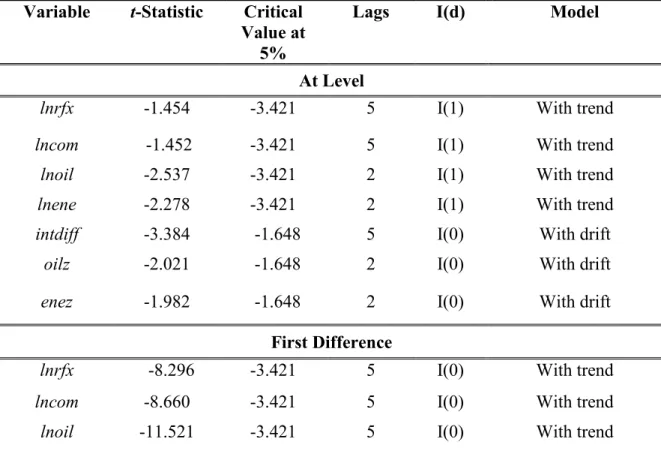
Table 1. Augmented Dickey-Fuller test ... 41

Table 2. Weak exogeneity test (1972/01-2011/09) ... 43

Table 3. lnrfx Granger causality test (1972/1-2011/9) ... 43

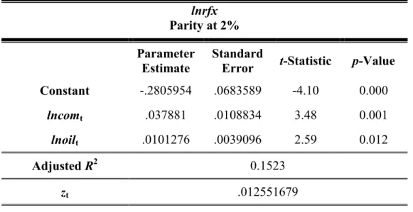
Table 4. Estimation of the long-run equation with lnoil when parity is at

2% ... 45

Table 5. Estimation of the long-run equation with lnoil out of 2% parity

... 46

Table 6. Estimation of the long-run equation with lnoil when parity is at

5% ... 46

Table 7. Estimation of the long-run equation with lnoil out of 5% parity

... 47

Table 8. Estimation of the short-run equation with lnoil out of 2% parity

... 49

Table 9. Estimation of the short-run equation with lnoil when parity is at

2% ... 50

Table 10. Estimation of the short-run equation with lnoil out of 5% parity

... 51

Table 11. Estimation of the short-run equation with lnoil when parity is at

5% ... 52

Table 12. Structural break tests (1972/01- 2011/09) ... 55

Table 13. Structural break tests for subperiod 1 (1972/01-1991/12) ... 55

Table 14. Structural break tests for subperiod 2 (1992/01-2011/09) ... 55

Table 15. Likelihood ratio test long run model (1972/01-2011/09) ... 56

(14)

xiv

Table A1. Estimation of the long-run equation with lnene when parity is

at 2% ... 65

Table A2. Estimation of the long-run equation with lnene out of 2%

parity ... 65

Table A3. Estimation of the long-run equation with lnene when parity is

at 5% ... 67

Table A4. Estimation of the long-run equation with lnene out of 5%

parity ... 67

Table A5. Estimation of the short-run equation with lnene out of 2%

parity ... 68

Table A6. Estimation of the short-run equation with lnene when parity is

at 2% ... 69

Table A7. Estimation of the short-run equation with lnene out of 5%

parity ... 70

Table A8. Estimation of the short-run equation with lnene when parity is

at 5% ... 71

Table A9. Durbin-Watson of the short-run equation ... 71

Table A10. Order selection criteria ... 71

Table A11. Granger causality test for parity vs. non-parity 2% and 5% 72

(15)

xv

LIST OF FIGURES

Figure 1. Canadian dollar and oil prices: 1999-2011 ... 13

Figure 2. Canadian dollar and commodity prices: 1999-2011 ... 14

Figure 3. Canadian dollar and oil prices: 1986-2013 ... 15

Figure 4. CAD/USD exchange rate and Purchasing Power Parity

(1960/01-2011/09 ... 17

Figure 5. CAD/USD exchange rate & interest rate differentials

(1972/01-2011/09) in US... 37

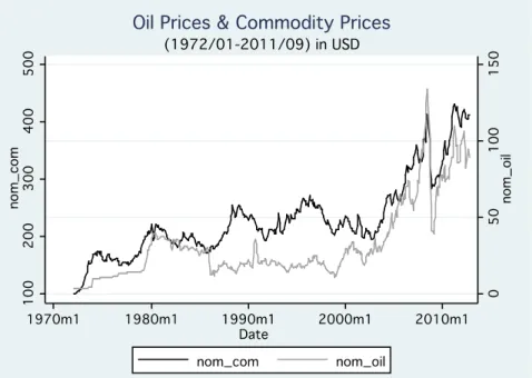
Figure 6. Oil prices & commodity prices (1972/01-2011/09) in USD ... 39

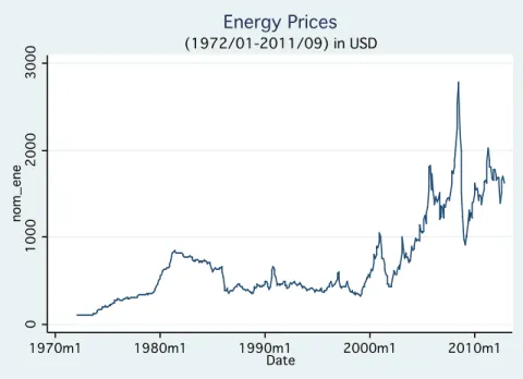
Figure 7. Energy prices (1972/01-2011/09) in USD ... 40

Figure 8. The lnoil residual of the long-term equation between

(1972/01-2011/09) ... 47

Figure 9. The lnene residual of the long-term equation between

(1972/01-2011/09) ... 48

(16)

(17)

1

1 INTRODUCTION

In the early 1990s, the Bank of Canada (thanks to Amano and van Norden (1993)) developed an exchange rate equation to determine and understand the driving forces of the CAD/USD exchange rate. The AvN equation was constructed on the basis that oil prices account for the movements of the CAD/USD exchange rate, with the underlying impression that the CAD/USD exchange rate moves in tandem with oil prices. The AvN equation has proven to be relatively robust at detecting the major shifts in the CAD/USD exchange rate between 1997 and 2002. Nevertheless, between 2003 and 2005 there was an abrupt appreciation of the Canadian dollar. The Canadian dollar strengthened by about 25 US cents and the Bank of Canada’s exchange rate equation then turned out to be unsuccessful in estimating the CAD/USD exchange rate. Previous studies have demonstrated the presence of a structural break in the determination of the CAD/USD exchange rate. Among them, Maier and DePratto (2008), Issa, LaFrance and Muray (2006) and Amano and van Norden (1995) stand out. The main objective of this thesis is to uncover the driving factor behind this structural break. Our most important contribution is the application of an error correction model which encompasses the effect of parity versus non–parity in the determination of the CAD/USD exchange rate.

The Bank of Canada has long acknowledged the causal link between oil prices and the CAD/USD exchange rate. It is of high importance to discover the driving factors of the movements of the CAD/USD exchange rate. For, understanding the underpinning factors of the CAD/USD exchange rate equation will help regulators to set the bank rate. It will also apprise monetary authorities of the most appropriate monetary policy to undertake.

Oil is not like any other good. It has a crucial importance because it enters as an input in the production and transportation of most other goods. Therefore, when its price rises, firms and consumers end up spending more money on oil. Since Canada is a net oil exporter, a rise in the price of oil implies a rise in the demand for the Canadian dollar at the international level. This increased demand for the Canadian dollar will translate itself into

(18)

2

an appreciation of the Canadian dollar unless it is counteracted by some other factor, like the anticipation of a future deprecation. The assumption in this study is that, in general, these anticipations exist when the Canadian dollar reaches parity with the American dollar. At parity, since this event has been rare and has not lasted very long since the early seventies, currency traders anticipate a depreciation and start selling their Canadian dollars. In that instance, ceteris paribus, the Canadian dollar reacts less to a given increase in oil prices. The respective monetary policies of Canada and the United States may also influence the relative value of the Canadian dollar, and these will be considered as well in our study.

The 1985 NAFTA Accord led to a significant deregulation of the natural gas industry and since the 1990s the energy sector in Canada has undergone a major development, as the production has almost doubled. Canada has become a world-class exporter of energy products, ranked 3rd largest producer of oil and 7th producer of natural gas worldwide. Moreover, Canada has the world’s third largest oil reserves. The CAD/USD bilateral exchange rate is of major importance because Canada and the United States share the greatest bilateral trade volume in the world. In addition, both countries share the same policies of floating exchange rate and open capital markets. Canada trades about three-fourths of its exports each year with the U.S. Since 1989 US-Canada Free Trade Agreement (FTA) and the 1994 North American Free Trade Agreement (NAFTA), the U.S. has become Canada’s major trading partner.1 We may then expect that this large trade will help us decipher the underlying factors of CAD/USD exchange rate.

Our methodology is inspired from the exchange rate equation developed by Amano and van Norden (1993) at the Bank of Canada. It is based on an error correction model. Stationary tests are used to verify whether the variables are non-stationary. Thereafter, the Engle and Granger two-step method is implemented to verify cointegration of the variables. Two long-term dynamics of the CAD/USD exchange rate are specified using two world commodity prices: one model involves oil prices and non-energy commodity prices, while the other contains energy prices and non-energy commodity prices. The interest rate

(19)

3 differential is included in the short-term equation in order to capture the short-term dynamics.

We further address the question of parameter stability. A variety of tests, such as the Likelihood ratio test, are implemented to check the stability of the exchange rate equation. We uncover the mystery of the structural break that occurs in the AvN equation by focusing on the presence of parity versus non-parity of the CAD/USD exchange rate as the break point. The results indicate that a structural break occurs when the CAD/USD exchange rate is at parity. The coefficients of the estimated parameters then tend to zero.

This thesis is organized as follows. Chapter 1 provides a brief introduction. Chapter 2 reviews the literature on exchange rate models. The literature is divided into two parts: The first one presents the major studies about the movement of the Canadian dollar, while the second one concentrates on exchange rate models related to other currencies, with more emphasis devoted to the Canadian dollar. Chapter 3 presents a concise overview of the fluctuations of the Canadian dollar, followed by a discussion about the fundamentals of the CAD/USD exchange rate in Chapter 4. The methodology is described in Chapter 5, where we present the error correction model and the various diagnostic tests that are used to assess the presence of a unit root and the stability of the parameters. In Chapter 6, the trends of all the variables in the model are presented through a graph. Finally, Chapters 7 and 8 exhibit the results and the conclusion, respectively.

(20)

4

2 LITERATURE REVIEW

2.1EXCHANGE RATE MODELS RELATED TO OTHER COUNTRIES

The literature on structural time series demonstrates that real shocks are a key factor of real exchange rate fluctuations. Baxter (1994), Huizing (1987) and Clarida and Gali (1994) employed the Beveridge-Nelson univariate and multivariate decompositions to demonstrate that most of the real US exchange rates2_{movements, originate from changes in permanent}

components or real shocks, as well as in temporary components, and may not follow a random walk. Work by researchers such as Lastrapes (1992) and Evans and Lothian (1993) used the Blanchard and Quah (1989) decomposition to reveal that much of the variance of both real and nominal exchange rates from a number of countries over the short and the long runs can be attributed to real shocks. The results observed in the structural-time series literature thus appear to be robust to both decomposition methods and currencies. This motivated some researchers to suggest that an unknown real factor may be the source of the persistent shifts in real equilibrium exchange rates.

In an effort of identifying this real factor, some authors studied the relationship between real domestic oil prices and real exchange rates of Germany, Japan and the United States. This has been undertaken by McGuirk (1983) who looked at real exchange rate of the G7 countries3_{. Krugman (1983a, 1983b) studied the US real exchange rate. Golub (1983)}

investigated the US dollar and the Deutsche Mark exchange rate. Rogoff (1991) examined the Yen/USD exchange rate, while Amano and van Norden (1995) found a link between oil prices and the movements in the CAD/USD real exchange rate. In this latter study, the authors suggested exploring the ability of oil prices to account for the movement of real exchange rate of other currencies. Hence, Amano and van Norden (1998) examined the relationship between the real domestic price of oil and the real effective exchange rates for Germany, Japan and the United States. They concluded that the real oil price absorbs

2_{USD/DM, USD/YEN, USD/POUNDS, USD/CAD.}

(21)

5 exogenous terms of trade shocks, and they substantiated the importance of terms of trade in determining real exchange rates in the long run.

Amano and van Norden (1995) tested for cointegration between exchange rates and oil prices using the Engle and Granger (1987) two-step approach. Their results provided a strong indication of cointegration between oil prices and the real effective exchange rates for Germany and Japan but not for the United States. They compared their findings with the Johansen-Juselius (JJ) test, which provides evidence of cointegration for the three above mentioned countries. Likewise, Amano and van Norden (1998) analyzed the relationship between oil prices and the U.S. real effective exchange rates over the post Bretton Woods period. They demonstrated that these two variables are cointegrated, and that the relationship runs from oil prices to exchange rates and not vice versa. In other words, they established that the price of oil Granger-causes the exchange rate. They further showed that the U.S. real effective exchange rate contains a unit root. Sadosky (2010) obtained that energy prices and U.S. real exchange rates are cointegrated, and his results are congruent with previous studies. Moreover, using a structural vector autoregressive model (SVAR), Akram (2009) demonstrated that a weaker US dollar results in higher oil prices.

Benassy-Query et al (2007) further confirmed these results. They showed that there is a unidirectional causality behavior running from oil prices to the EURO/USD exchange rate. Chen and Chen (2007) indicated that the inclusion of real oil prices can considerably improve the ability to forecast exchange rates of the G7 countries. This leads to conclude that the existing “out-of-sample” causality runs from oil prices to exchange rates. The same results were obtained by Coudert et al (2008) who further suggested that the relationship between oil prices and the U.S. effective exchange rate is transmitted through the U.S. net foreign asset position.

Though Lizardo and Mollick (2010) also observed that crude oil prices significantly account for the movements in the exchange rate of the U.S. dollar against other currencies, they concluded that the effect of oil price changes on the exchange rate of a country’s currency varies depending on whether the country is a net oil exporter or importer.

(22)

6

Other authors such as Akram (2004) and Wang and Wu (2012) addressed the question of the existence or nonexistence of a nonlinear relationship between energy prices and exchange rates. Akram (2004) examined the possibility of a nonlinear dependence between the krone/ECU exchange rate and oil prices. His results demonstrated the presence of a negative relationship between oil prices and the Norwegian currency exchange rate. His model reveals that allowing for nonlinearities can significantly improve forecasting exchange rate models. This model is capable of performing well in-sample, and extensively improves the estimate of a random walk and an equivalent model but with linear oil price effects. Similarly, Wang and Wu (2012) investigated the issue of nonlinearity between the U.S. exchange rate dollar and crude oil prices. They found a structural break marked by the recent financial crisis. Before the financial crisis, there was a unidirectional linear causality going from petroleum prices to exchange rates, whereas after the financial crisis, their results depict a bidirectional nonlinear causality between exchange rates and petroleum prices.

(23)

7 2.2EXCHANGE RATE MODELS RELATED TO THE CANADIAN DOLLAR

In 1970, Canada reverted to a floating exchange rate regime. Since then, numerous studies have attempted to determine the key determinants of the Canadian dollar. Meese and Rogoff (1983) found that sticky price and flexible price monetary models, as well as portfolio balance models, fail to outclass a random walk model. They were the first to conclude that monetary variables such as the interest rate differential, the inflation rate differential and the current account have little effect on the real effective exchange rate. Another mainstream of economists studied the relationship between the real exchange rate and the terms of trade. Among these scholars are Dornbusch (1980), Neary (1988) and Edwards (1989). They discovered that the terms of trade may account for the relative price of non-traded goods in the long run. This effectively entails that the terms of trade are cointegrated with the real exchange rate. Other researchers, such as Engel (1999), Burstein et al. (2005) and Betts and Kehoe (2006), demonstrated that the relative price of traded goods accounts for the movement of the real exchange rate. Using out-of-sample data, Amano and van Norden (1993a, 1995) found a cointegrating relationship between the real exchange rate and the terms of trade. They concluded that much of the variation of the exchange rate can be explained by the terms of trade variable, particularly over long horizons. Their methodology is based on an error correction model. Their model appears to outperform the random walk out-of-sample process. Although there are periods during which their exchange rate equation seems to do worse than the random walk models, the AvN equation generally has a lower mean-squared forecast error than random walk models. Whilst Meese and Rogoff (1983) established that no other known model could make better predictions than a random walk process, Amano and van Norden (1993a, 1995) found a decade later that their equation (AvN) substantially improves the forecast, and is proven to be a better estimation than a random walk model.

The oil shocks of the 1970s spurred several studies on how the exchange rate in small open economies might react to commodity price shocks. Some authors, like Neary and Purvis (1982), Bruno and Sachs (1982) and Corden (1984), discussed the implications of the Dutch

(24)

8

disease for commodity producers. Amano and van Norden (1993a, 1995), Chaban (2010), Gauthier and Tessier (2002), Laider and Aba (2001) and many others, showed that the long run value of the Canadian dollar may be driven by the terms of trade. It is also worthwhile mentioning the works of Issa, LaFrance and Murray (2006), Obstfeld and Rogoff (2000), and Chen and Rogoff (2003).

Amano and van Norden (1993a, 1995) split the terms of trade into energy and non-energy, and identified a cointegrating relationship of each of these parts with the real CAD/USD exchange rate. This is not consistent with the results presented by Obstfeld and Rogoff (2000), who argued that terms of trade shocks are not easily traceable due to different pricing mechanisms and an incomplete pass-through. Most of the current literature does not adhere to this latter view. In addition, Chen and Rogoff (2003) argued that the relationship between non-energy commodity prices and the real CAD/USD exchange rate does not hold if the variables are assumed to be trend stationary.

Gauthier and Tessier (2002) examined the question of whether supply shocks impact the CAD/USD real exchange rate. Their findings suggest that in the long run, 61% of the movement of the exchange rate is attributable to supply shocks. The short-term dynamics are driven by commodity price shocks and transitory shocks, but commodity price shocks do not explain the long term variations of the exchange rate. These results are in contrast with Amano and van Norden (1993a, 1995)’s conclusions. The AvN equation is constructed on the premise that commodity prices are the long run determinant of the exchange rate. Gauthier and Tessier (2002) argued that the long run specification built by Amano and van Norden (1993a, 1995) “overemphasizes” the importance of commodity prices by focusing only on the commodity prices as fundamentals. Since Gauthier and Tessier (2002)’s model provides a richer set of shocks, the emphasis on commodity prices is reduced.

Because Amano and van Norden (1993a, 1995)’s work proved to be fruitful, further studies analyzed the stability parameters of the relationship between the Canadian dollar and energy and non-energy commodity prices. They established that the relationship is not stable over

(25)

9 time. Studies on this topic include Issa, Lafrance and Murray (2006), DePratto and Maier (2008), Chaban (2010), Laider and Aba (2001) and Bayoumi and Mühleisen (2006).

Laider and Aba (2001)’s findings are consistent with Amano and van Norden (1993a, 1995) in the sense that the Canadian dollar is regarded as a commodity currency. Laider and Aba (2001) explain that the Canadian dollar will persist in being viewed as a commodity currency as long as Canada remains a major commodity exporter. They confirmed Amano and van Norden (1993a, 1995)’s results to the effect that short-term fluctuations of the CAD/USD real exchange rate can be captured by the interest rate differential between the two countries. They replicated the AvN equation, but included three separate coefficients, one for each of the 1970s, 1980s and 1990s variables. They noticed that the sensitivity to commodity prices diminishes from decade to decade. Furthermore, they observed that energy prices do not play a major role in the model after the 1990s.

Amano and van Norden (1993a, 1995) also found that over their data set (1973-1993) oil price movements could explain the depreciation of the Canadian dollar in the long run. Picking up where Amano and van Norden (1993a, 1995) had left off, Issa, Lafrance and Murray (2006) implemented different specifications of the AvN equation by allowing for structural breaks using a richer sample period (1973Q1-2005Q4). They introduced a new indicator I(t>τ) in the exchange rate equation to allow for the break that occurred in 1993. Indeed, before 1993 a rise in energy prices resulted in a depreciation of the Canadian dollar, whereas since 1993 a rise in energy prices causes an appreciation of the Canadian dollar. As opposed to Amano and van Norden (1993a, 1995), Issa, Lafrance and Murray (2006) observed that the effect of energy prices turned positive in the early 1990s. Although they recognized that their equation can be improved, the ILM (for Issa, LaFrance and Murray) equation can account for most of the Canadian dollar’s appreciation since 2003. Overall, their equation appears to perform better than the AvN equation.

Several researchers focused their approach on the relative composition of trade over time in the exchange rate equation. Among these economists are Bailliu and King (2005), Bayoumi, Faruqee and Lee (2005), Bayoumi and Mühleisen (2006) and DePratto and Maier (2008).

(26)

10

Bayoumi and Mühleisen (2006)’s approach differs from that of Bailliu and King (2005) in two aspects. First, the short-term dynamics take into account the “contemporaneous” rate of change of commodity prices, whereas the earlier specification relied only on the error correction mechanism to adjust it. Secondly, Bayoumi and Mühleisen’s model takes into consideration the ratio of commodity trade balance to non-commodity imports.

Moreover, Bayoumi and Mühleisen (2006) followed Bailliu and King (2005)’s suggestion, which consists in allowing the coefficient of energy to change in 1990Q1, in order to reflect the increase of energy exports in the Canadian trade. This modification provided a better data fit. DePratto and Maier (2008) obtained similar results. They added a dummy variable and ran tests to check for parameter stability between 2002 and 2004 for each year. Their results indicate evidence in favor of structural breaks around 2002/2003.

DePratto and Maier (2008) made advances by employing two approaches: the first one is based on Bayoumi and Mühleisen (2006)’s work and highlights the importance of the export basket, while the second one associates to the energy variable a weighting factor of the ratio of energy exports minus energy imports to the GDP, as well as a weighting factor to non-energy commodity prices. They referred to this approach as “controlling for commodity dependency”, as it aims to reflect the dependency of the Canadian economy on energy and non-energy commodity prices. DePratto and Maier (2008) compared the “baseline specification” from Issa, Lafrance and Murray (2006), the “controlling for export intensity” from Bayoumi and Mühleisen (2006), and their “controlling for commodity dependency” approaches. They concluded that the “controlling for export intensity” and “the controlling for commodity dependency” approaches provide more stable parameters than the “baseline specification” approach.

The results of Bachetta and van Wincoop (2004) contradicted previous findings. They explored an exchange rate model driven by trading activities of a large group composed of informed market participants. They suggest that the relationship that exists between energy

(27)

11 commodity prices and the real exchange rate may be attributed merely to the fact that most foreign exchange traders are focusing on the price of oil in their decisions to buy or sell the Canadian dollar. They also claim that financial markets play a significant role, at least in the short-term volatility of the Canadian dollar. Murray, Norden and Vigfusson (1996) addressed the same question by estimating a Markov-switching regime model. Two different regimes were estimated: a fundamentalist regime based on the terms of trade, and a chartist regime. The chartist trading strategy relies on the assumption that traders’ activities are guided by the observation of historical prices to forecast future trends. Murray, Norden and Vigfusson (1996)’s results demonstrated that the fundamentalist regime is predominant when there are large changes in the exchange rate. When the changes are small, the chartist regime prevails.

Other literature moved away from the issue of robustness and explored the presence of deterministic trends and the question of lag order. Two aspects differentiate Chaban (2010)’s paper from Issa et al (2006). First of all, Chaban (2010)’s research paper includes deterministic trends in the analysis and allows for structural breaks in those trends. Chaban (2010) established that one should take into account deterministic trends in the analysis, thus challenging the assumption of no deterministic trend in Amano and Van Norden (1993a, 1995). Chaban’s paper did not find enough evidence to reject stochastic trends in the analysis. Kollman (1993) considered a deterministic trend and concluded that whether non-energy terms of trade are trend stationary or not depends on the lag order.

Similarly, the NEMO equation, built by Helliwell, Issa, Lafrance and Zhang (2005), moved away from the question of robustness and examined the inclusion of other variables in an error correction model. NEMO is able to track the major appreciation of the Canadian dollar from 2003 to the third quarter of 2004. This equation incorporates two main long-term determinants: the relative labor productivity differentials between Canada and the United States and a split between the real energy and non-energy commodity prices. The short-term dynamics that are captured by this model are the Canada-US short-term interest rate

(28)

12

differentials, the evolution of the US dollar relative to other currencies, and a measure of risk perception in international markets.

(29)

13

3. ABOUT THE MOVEMENT OF THE CAD/USD EXCHANGE

RATE

Canada moved to a flexible exchange rate on June 1st, 1970. Since then the Canadian dollar has reached an all-time low of CAD 1 = USD 0.6179 on January 21st, 2002 and an all-time high of CAD 1 = USD 1.1030 on November 7th, 2007.

From 1991 to 2002, the Canadian dollar weakened substantially compared to its US counterpart. In 1991, it was worth 89 US cents, while by 2002 it had dropped to 61 US cents. We began to hear about “the long term decline” of the Canadian dollar, but this was illusory. The reach of an all-time low at the beginning of 2002 could be explained by the economic slowdown that took place in 2001 and the fact that The Bank of Canada stimulated the economy through expansionary monetary policy to get the Canadian economy back on track. Indeed, Amano & van Norden (1993) found that the monetary policy has short-term effects but not long-term effects. Accordingly, the expansionary monetary policy in 2001-2002 only had a brief effect that led to a last leg down of the CAD/USD exchange rate.

By the end of 2002, the Canadian dollar began its takeoff and continued its ascent to reach parity with the US dollar in 2007, and even enjoyed the above mentioned all-time high in November of that year. This record coincided with an economic slowdown in the United States in 2007, followed by the Great Recession (which was marked by US housing and financial markets turmoil).

Figure 1 depicts the relationship between the Canadian dollar and oil prices over the 1999-2011 period. Blue points are used to represent data gathered when the price of oil stood below USD 85/barrel. Green points denote data collected when oil prices were above that threshold. The dash-dotted black line corresponds to the fitted linear regression of the blue data points. This positive linear movement between the price of oil and the Canadian dollar was observed during most of the 2000’s. An increase in the price of oil translated into a

(30)

14

proportional appreciation of the Canadian dollar versus its US counterpart. When the price of oil reached USD 80/barrel in September 2007, the Canadian dollar was nearly at parity with the American dollar. The price of oil continued to increase and the linear relation observed for almost six years by then remained valid for a few more months. But

4

Figure 1. Canadian dollar and oil prices: 1999-2011.

while the price of oil continued its ascent, the value of the Canadian dollar remained close to parity with the American dollar. Clearly, the fitted regression line fails to reflect the relationship between oil prices and the CAD/USD exchange rate when oil prices exceed USD 85/barrel or when the Canadian dollar is significantly above parity. It seems that around parity there is a breakdown point between the price of oil and the Canadian dollar. Figure 2 shows the relationship between the Canadian dollar and commodity prices between

4_{http://worthwhile.typepad.com/worthwhile_canadian_initi/2011/03/parity.html#more}_{last visit on}

(31)

15 2000 and 2011. The dash-dotted line is the fitted regression line of the blue points, which represent the commodity price index of the Bank of Canada in US dollars vs. the CAD/USD exchange rate. It is similar to the previous graph, which exhibits the relationship between oil prices and the Canadian dollar.

5

Figure 2. Canadian dollar and commodity prices: 2000-2011.

It can be noticed that the linear relationship holds when the commodity price index is less than 620 USD and the exchange rate is below unity. Once the value of the Canadian dollar moves above unity, this linear relationship does not hold anymore. It seems that there is kink at the point where parity is reached. Otherwise, at a commodity price index above 620 USD one would predict a Canadian dollar well above parity against the American dollar.

The object of this paper is to revisit the relationship between CAD/USD exchange rate and oil/energy prices, and to examine whether this relationship is broken over time by testing the

5_{http://worthwhile.typepad.com/worthwhile_canadian_initi/2011/03/parity.html#more}_{last visit on}

(32)

16

parameters’ stability. In the model employed, the main factors that determine the CAD/USD exchange rate are commodity prices and oil/energy prices. This has proven to be fruitful in the last decades. We are interested in oil and energy prices as they play a major role in the Canadian economy. Energy products are the largest category of Canadian exports segments. They accounted for 23% of the total exports and about 10% of the total imports in 2012. It is also noteworthy to mention that 62% of Canada’s imports come from the United States and that 73% of Canada’s exports are bound for the United States.6

Figure 3. Canadian dollar and oil prices: 1986-2013.

Figure 3 depicts the relationship between oil prices and the CAD/USD exchange rate described above over a larger data span. (The daily data for oil was available only since 1986.) This figure confirms that the same pattern occurs over a larger sample, namely that

6_{http://www5.statcan.gc.ca/bsolc/olc-cel/olc-cel?catno=57-601-XIE&lang=eng#formatdisp}_last

(33)

17 once the parity zone between the CAD and USD is reached, an increase in oil prices does not lead to an increase in the CAD/USD exchange rate in the same proportion than before reaching that parity zone.

(34)

18

4 F

UNDAMENTALS OF THE EXCHANGE RATE

4.1PURCHASING POWER PARITY AND THE LAW OF ONE PRICE

The law of one price states that goods and services must sell for the same price when comparing prices in a single currency, regardless of which country the goods and services are sold in. According to this law, consumers and businesses will adjust themselves so that the prices of goods and services in Canada will be equal to the prices of the same goods and services in the United States multiplied by the CAD/USD exchange rate (see Macdonald (2012)). In practice, there is little evidence to support the law of one price, as competitive markets face transportation costs and barriers to trade (such as tariffs). This law is valid only for tradable goods and services. Let’s suppose the CAD/USD exchange rate is CAD 1 = USD 0.99. If a t-shirt sells for USD 10 in the United States, then this t-shirt should cost CAD 10.10 in Canada, assuming that the law of one price holds. Indeed, this is equal to the given CAD/USD exchange rate multiplied by the USD price: CAD 1 / USD 0.99 * USD 10 = CAD 10.10. The law of one price provides a link between the relative cost of goods between two countries and their respective exchange rate. It follows that the CAD/USD exchange rate is given by the ratio CAD Price / USD Price = PCA/ PUS.

The law of one price applies to a single product or service, whilst the Purchasing Power Parity represents an aggregate measure of representative goods and services that are consumed. It provides a measure of the price levels between two countries. The PPP theory foreshadows that an increase in the domestic purchasing power results in a proportional appreciation of the domestic currency, and vice versa. Hence, PPP theory predicts that the CAD/USD exchange rate satisfies

PCA = ECA/US * PUS,

where ECA/US stands for the CAD/USD exchange rate. The PPP theory also implies that the

(35)

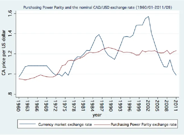
19 currency. The CAD/USD PPP exchange rate provides a theoretical measure of the CAD/USD exchange rate based on observed prices as long as these latter adjust between the two countries. In the real world, though, the currency market exchange rate is generally not equal to the Purchasing Power Parity ratio. As Figure 4 shows, in the 1960s the market exchange rate was above the Purchasing Power Parity exchange rate. In the early 1970s they crossed each other and assumed opposite relative positions until 1981/1982.

Figure 4. CAD/USD exchange rate and Purchasing Power Parity (1960/01-2011/09).7

The CAD/USD Purchasing Power Parity exchange rate and the CAD/USD exchange rate move in the same direction over the long term. Over the short term, however, they may move in opposite directions, as Figure 4 exemplifies over numerous time intervals.

7

(36)

20

It was noted by Lafrance and Schembri (2002) that the Purchasing Power Parity is not the best determinant of the currency exchange rate for a number of reasons:

 The large discrepancy in the price levels between Canada and the US represents the costs of non-tradable goods and services (chiefly labor and land) which cannot adjust to equate the prices of a national basket.

 Traded goods are usually subject to taxes, tariffs and transaction costs.

 The real exchange rate is not constant. In the short run, it is influenced by money and “asset market shocks”. In the long run, it is affected by persistent real shocks. With this in mind, this thesis explores the effect of a real shock, namely the change induced in the real CAD/USD exchange rate by a change in oil or energy prices.

Even though the United States and Canada have similar economic structures, their price level difference might not be explained by the currency exchange rate. International financial flows play an important role in determining the price level of a given country.8

Baldwin and MacDonald (2009) found that between 1961 and 2000 the GDI deflator and the CAD/USD exchange rate both moved down, while they both moved up after 2000. Nevertheless, as we observed in Figure 4, there are several time intervals where the PPP and the currency exchange rate moved in opposite directions. Their study also demonstrates that in the long run the levels of the PPP exchange rate and the CAD/USD exchange rate are quite different.

As shown in Figure 4, the market exchange rate is more volatile than the PPP exchange rate. Hence monetary policy has no long run influence on the real exchange rate. According to the PPP theory, countries with different inflation rates adjust their bilateral exchange rate to eliminate the inflation rate differences in the long run. Consequently, PPP is advantageous in determining the exchange rate only when monetary shocks predominate; for instance, when monetary policies account for different inflation rates between countries. However, PPP

8_{Purchasing Power Parities and real expenditures, United States and Canada, 2002 to 2009. 2011. Statistics}

(37)

21 does not consider the effect of real shocks to the real exchange rate (LaFrance and Schembri (2002)).

The empirical evidence of the PPP theory is limited. Econometric tests of PPP theory have evaluated the extent to which the real exchange rate tends to return to a mean or to an average level. Froot and Rogoff (1995) concluded that there seems to be a convergence of the PPP in the long run, but this result emerges from data sets that use at least some fixed-rate data. They suggested exploring the convergence to PPP under floating exchange fixed-rates, when more years of floating exchange rate data become available. Johnson (1992) used time horizons of 50 to 80 years for the PPP and the Canadian dollar. Both studies assert that the PPP is detectable in about 50 years. This leads us to think that in the long run monetary factors have a strong influence on the real exchange rate, and that the exchange rate tends to move to an average level when examined over very large samples.

It is concluded that when shocks are monetary in nature, the exchange rate follows the relative PPP in the long run. In the long run, a monetary shock will influence the general purchasing power of a currency, which equals the currency’s value in terms of domestic and foreign goods. When disturbances take place in the output market, the exchange rate might not follow to the relative PPP, even in the long run. This explains why the exchange rate equation considered in this thesis involves oil and energy prices.

4.2REAL EXCHANGE RATES AND INTEREST RATE DIFFERENTIALS

Empirical investigations have been conducted by researchers to determine whether there is a relationship between the interest rate differential and the real exchange rate. Meese and Rogoff (1988) used the sticky-price model and failed to find evidence of a statistical link between the interest rate differential and the real exchange rate. Other economists such as Edison and Paul (1993) used cointegration tests and error correction models and found little evidence of a long-term relationship between the real exchange rate and the interest rate differential. These findings were akin to the results of Campbell and Clarida (1987) in the

(38)

22

sense that “changes in the real exchange rates are persistent and more volatile than real interest rate differentials,” leading to the observation that the expected real interest rate differential exerts little influence on the variation of the real exchange rates.

On the other hand, Baxter (1993) found evidence of a relationship between the real interest rate differential and the real exchange rate. Baxter employed band-spectral methods. Her results suggested that the strongest relationship between the real interest rate differential and the exchange rate is present at low trend and business cycle frequencies. At high frequencies (cycles of 2-5 quarters), no relationship was found. Baxter’s findings contribute to understand why previous researchers failed to find a statistically significant relationship between these variables: they employed a filter which attributed most of the weight on the highest frequency elements of the data. Baxter (1993) revised the previous standard theory based on the uncovered interest rate parity and ex ante purchasing power parity and found little statistical link. Baxter (1993) built a model to evaluate the relationship between the real exchange rate and the real interest rate differential. The model looks at the temporary and the permanent components of the real exchange rate by the use of univariate and multivariate Beveridge-Nelson time series decompositions. Her results provided an indication of a strong correlation for multivariate measures. Conversely, when assessing the temporary component of the real exchange rate, the real interest rate differential did not have a significant influence on the movements of the real exchange rate.

According to Baxter, the link between the real interest rate differential and the real exchange rate is only attributable to the temporary component of the real exchange rate and most of the movement of the real exchange rate is due to the permanent component. The statistical link between the real exchange rate and the interest rate differential remains then very weak. In fact the relationship between temporary components and the real exchange rate is in itself very weak. This explains why previous researchers did not find a statistical link between these variables. Baxter (1993) attributed most of the movement of the temporary component of the real exchange rate to the “unobserved risk premium from the open interest parity condition”.

(39)

23 Previous studies such as Meese and Rogoff (1988) and Campbell and Clarida (1988) investigated the empirical linear relationship between interest rate differentials and the real exchange rate. They did not find a link between these variables. However, according to Baxter (1992), their assumptions between these variables were not corroborated with the data.

On the other hand, while Baxter (1992) and Meese and Rogoff (1988) explained that their failure to find a cointegrating relationship between interest rate differentials and the USD real exchange rate9 is due to an omitted real variable, Amano and van Norden (1998) provided empirical evidence to support otherwise. Indeed, they explained that the interest rate differential is not part of any long-run relationship with the USD real exchange rate. A relationship between these two variables is only present in short-run exchange rate movements. Hence, the single exchange rate equation presented in this thesis is based on the findings of Amano and van Norden (1998), in which interest rate differentials help explain short-term fluctuations of the CAD/USD exchange rate.

Moreover, Nakagawa (2001) employed an alternative approach by including nonlinearity in real exchange rate variations and evaluated its theoretical and empirical implications for the link between the real interest rate differential and the real exchange rate. Nakagawa (2001) augmented the Mundell-Fleming-Dornbusch (M-F-D) model to allow for threshold nonlinearity specification. The nonlinearity threshold allowed for nonlinear price adjustments, such as the consideration of transaction costs and other uncertainties, which led to a “band of inaction” or a “no-arbitrage region”. Given the above mentioned evidence of a possible impact of interest rate differentials on exchange rates, we will also consider this variable in our empirical analysis.

9

Amano and Van Norden (1998) used three different measures of the interest rate differential: USD versus Japan, USD versus Germany and a weighted measure to reflect the effective real USD real exchange rate.

(40)

24

5 M

ETHODOLOGY

10

In this research we have conducted some statistical tests on the variables under consideration. Initially, the stationarity/nonstationarity of the variables was assessed. Given the observed nonstationarity, cointegration tests were performed. Finally, Granger causality tests were used to help select the appropriate error correction model, and structural stability tests were conducted. The following section presents the various methodologies used in our analysis.

5.1UNIT ROOTS AND REGRESSION RESIDUALS

One has to be very careful when working with time series data. In general monetary variables tend to be nonstationary. This has its own implications and requires a particular attention. We are going to present the different scenarios that researchers are confronted with. Moreover, in this section we are going to explain why cointegration methods have been explored in this thesis.

Consider the regression equation

(1) The classical regression has to satisfy three conditions in order to be valid:

1. Both sequences and must follow a stationary process. 2. The errors must have a zero mean.

3. The variance must be finite.

Granger and Newbold (1974) generated two sequences and as two independent random walks to evaluate the effects of not satisfying the stationarity assumption, by using the following formulas:

10

The methodology is based on Enders, W. (2004) Applied Econometric Time Series (2nd Edition) Wiley,

(41)

25 (2) (3) where and exhibit a white noise process and are independent of each other.

If the variables are nonstationary, we are faced with what Granger and Newbold (1974) called a spurious regression. This type of regression has higher R2 and t-statistics and it displays a high degree of autocorrelation, which might lead to an erroneous interpretation of the data. The regression output might be misleading because the least-square estimates are not coherent and the traditional tests of statistical inference do not hold.

Let be the residual series. Granger and Newbold (1974) showed that the regression’s results are meaningless if the residual series are nonstationary. Because we know that are independent of each other, equation (1) or any relationship between these two variables is not reliable and thus spurious. Now let’s rearrange the equation so that is on the left and rewrite (1) as

Given that and are generated by (2) and (3), let be the initial conditions. Then ∑ ∑

As t increases the variance of the error tends to infinity. Furthermore, it can be noticed that the error has a permanent component such that for all . Hence, one of the

basic assumptions of any t-test, F-test, or R2 values will be violated and their values will be invalid. It is apparent, that residuals from a spurious regression will display a high degree of autocorrelation.

Under the null hypothesis in which , the generating process in (1) is given by . Since is integrated of order one, it ensues that is integrated of order one under the null hypothesis. Nevertheless, the fact that the error is a unit root process

(42)

26

contradicts the main assumption of the distributional theory underlying the use of OLS. Indeed, Phillips (1986) concluded that the larger the sample, the higher the probability to mistakenly conclude that .

There are four cases to consider when working with nonstationary variables: Case 1

Both and are stationary. The classical regression is then suitable. Case 2

and are integrated of different orders. Any regression or relationship between these

two equations will be pointless. Case 3

Both sequences and are integrated of the same order and the residual sequence has a stochastic trend. Since all the errors from the resulting regression are permanent in this case, the regression is spurious and any estimation from such a regression is meaningless. In this scenario, it is more appropriate to estimate the regression equation using the first difference of the given sequences. The first difference of (1) is

.

By taking the first difference of , and , each sequence is stationary since each one contains a unit root.

Case 4

If the nonstationary sequences and are integrated in the same order and the residual sequence is stationary. In this case, and are said to be cointegrated.

(43)

27 From the preceding discussion we know it is crucial to determine whether the variables in question are stationary or non-stationary. But if the considered process has a unit root, then it is a nonstationary time series. We now present the Dickey-Fuller test. This latter is used to test for the presence of a unit root.

Consider the equation

.

Subtract from each side of the equation in order to obtain the equivalent form

where . Since testing whether is equivalent to testing if , Dickey-Fuller tests, which are used to test the hypothesis , thus assess the presence of a unit root. This is done using three different regression equations:

(4) (5)

(6)

The first regression equation (4) is a pure random walk, whereas (5) and (6) each contain a deterministic element and , respectively). Equation (5) includes a drift or an intercept, while equation (6) adds a drift and a linear time trend.

The three regression equations comprise the parameter . If , then the yt sequence

contains a unit root.

The test consists in estimating one of the three regression equations via the OLS method. This allows us to obtain the estimated value of and the associated standard error. If =0, then the series has a unit root and is difference stationary. The next step is to compare the corresponding t-statistic with the critical value in order to decide whether to accept or reject the null hypothesis =0. If the t-statistic is greater than the Dickey-Fuller critical value, then the null hypothesis is not rejected and a unit root exists. If the t-statistic is less than the Dickey-Fuller critical value, then the null hypothesis is rejected and a unit root does not

(44)

28

exist. Note that the critical value of the t-statistic is contingent on whether the regression equation contains an intercept and/or a trend, as well as on the sample size.

EXTENSION OF THE DICKEY-FULLER TEST

The Dickey-Fuller test only takes into account the possibility of a single unit root. And not all the variables can be represented using a first-autoregressive process. Hence, the Dickey-Fuller test has been adapted to consider higher-order processes. This test is known as the

Augmented Dickey-Fuller (ADF). The Augmented Dickey-Fuller test considers a p-th

order autoregression which has p characteristic roots; if there are m p unit roots, the series has to be differenced m times to achieve stationarity.

Consider the p-th order autoregressive process:

In a similar manner to the Dickey-Fuller test, add and subtract to get

( )

Next, add and subtract to get

( ) Continuing in this manner we obtain

∑ where ∑ and

(45)

29 ∑

Note that it is not possible to estimate and its standard error unless all of the autoregressive terms are included. Hence, it is very important to select the appropriate lag-length in order to represent the true data-generating process. In this thesis, we used the Akaike Information Criterion (AIC).

5.2COINTEGRATION

In this section we are going to look closely at the definition of cointegration. The augmented Dickey-Fuller presented in the previous section allows us to confirm that our long-term variables lnoil, lnene and lncom11 follow a nonstationary process. At this point, the variables in question do not revert to a long-term equilibrium, making it difficult to construct a model because the variables can behave arbitrarily and differently. In order to circumvent this, we will use Engle and Granger definition of cointegration to show that it is possible to find a linear combination of nonstationary variables.

The term cointegration refers to a linear combination of nonstationary variables.

Let and represent the vectors ( ) and , the long-run equilibrium being . Any discrepancy from the long-run equilibrium is called the equilibrium error, denoted by , so that

If the equilibrium is significant, then the equilibrium error process is stationary. The term equilibrium refers to Engle and Granger (1987)’s use of the term. The equilibrium can be causal, behavioral, or a reduced-form relationship. Engle and Granger defined cointegration as:

(46)

30

The vectors are said to be cointegrated of order d, b, expressed by

if

1. All the elements of are integrated of order d.

2. There exists a vector such that a linear combination

is integrated of order ( ) where .

THE ENGLE AND GRANGER METHODOLOGY

Step 1

Pretest the variables using the Augmented Dickey-Fuller test to determine whether the variables are stationary or nonstationary. If it is possible to conclude that the variables are nonstationary, then we can proceed to the Engle and Granger methodology of cointegration.

Step 2

If the results of step 1 indicate that all the variables are nonstationary, then we can estimate the long-run relationship using the OLS regression method. If the variables are cointegrated, the OLS regression method yields a consistent estimator of the respective parameters and so on.

Consider the following two regression equations:

and

where

= CAD/USD real exchange rate = commodity prices in Canada = energy prices in Canada = oil prices (WTI).

(47)

31 Estimate the two long-run regression equations below. In order to establish if the variables are actually cointegrated, we represent the residual sequence from these two equations by and . These two series and are the estimated values of the deviations from the long-run relationship.

Step 3

Now that we have already established in step 1 that all the variables from the long-run regression equation are nonstationary. In order to be able to conclude whether there is cointegration or not, we need to determine if the residuals from the two regression equations below are stationary. Similarly to step 1, we will perform the Dickey-Fuller test to test if the residuals and are stationary. This will take the form of:

,

Since both residuals are coming from a regression equation, there is no need to include an intercept term; the parameter of interest is . If the residual from each regression equation are found to be stationary, it is possible to conclude that the and are cointegrated of order (1,1) and that and are cointegrated of order (1,1). More precisely, the rejection of the null hypothesis implies that the residuals sequences of each regression equation are stationary.

Note that because the values of the parameters are estimated values of the true values, we only know the estimated value of the and . Thus, we would not use the ordinary critical values of the Dickey-Fuller table, but the critical values for the Engle-Granger cointegration test.

To sum up, in order to conclude that the variables are cointegrated, we have to reject the null hypothesis , so the residual sequence is stationary.

(48)

32

Since we have already concluded that there is cointegration. We can proceed to estimate the error-correction model, which corresponds to the short-term equation. The magnitude of the residuals and is the deviation from the long-run equilibrium in period (t-1). Hence, we will incorporate the residuals obtained in step 2 in the short-term estimation. The estimated error correction model (ECM) will then take the following form:

It is important to notice that the short-term regression equation incorporates the interest rate differential (intdiff) which was not included in the long-term regression. The variable intdiff is considered to have only a short-term effect, thus it is not included in the long-term regression equation.

Finally, the variables are all expressed in logarithms as they can directly be interpreted in terms of elasticity or ratio.

Step 5

This step attempts to assess whether the error correction model is suitable. We conducted a weak exogeneity test. We start by regressing

.

We capture the residual from this regression, to include it in the test for each variable, in the following manner:

, Rule of decision:

(49)

33 H0 : the null hypothesis is rejected and the variable is not weakly exogenous.

5.3GRANGER CAUSALITY AND THE REAL EXCHANGE RATE

The Granger causality consists in testing whether the lags of one variable enters into the equation for another variable.

Consider the following n-equation VAR

[ ] [ ] [ ] [ ] [ ], where

= the parameters representing intercept terms, = the polynomials in the lag operator L.

The polynomials are all of the same degree. The individual coefficients of

are denoted by … . The terms denote the white-noise disturbances that

may be correlated.

comprises the coefficients of lagged values of variable j on variable i. Let’s suppose

we have a two-equation model with p lags and the variables and . We want to determine whether improves the forecasting performance of . We can say that

does not Granger cause if and only if all of the coefficients of are equal to zero. Consequently, if does not improve the forecasting performance of , then does not

(50)

34

Granger cause . If all the variables are stationary, under the restriction of the F-test, the

Granger causality test can be verified as follows:

.

It should be noted that the Granger causality test does not examine contemporaneous exogeneity. Granger causality indicates the effects of past values of on the current

value of . Hence, Granger causality provides evidence on whether current and past

values of improve the estimated values of .

Rule of decision:

Ho: does not Granger cause ( / / / ). If p-value > 0.05, then

we cannot reject the null hypothesis.

H1: does Granger cause ( / / / ). If p-value < 0.05, then we

reject the null hypothesis in favor of the alternative hypothesis.

In our analysis, we look at causality between exchange rates and oil prices, energy prices, commodity prices and the interest rate differential.

5.4TESTS FOR PARAMETER STABILITY

This section describes the various tests performed to verify if the relationship between oil or energy prices and the exchange rate changes during periods of near-parity.

1) F-test

1. Create a dummy variable regressor, denoted by , which is coded 1 at parity and 0 otherwise (i.e. at non-parity):

(51)

35 {

2. Run the following regressions:

and . 3. Hypothesis testing: 4. Rule of decision

The null hypothesis is rejected at the 5% significant level. There is insufficient information to support a conclusion.

2) Predictive Chow test

We want to test whether there is a structural change when the CAD/USD is at parity with the USD. Let denote the period at parity and the period at non-parity. The unrestricted regression that allows the coefficients to be different may be written as

[ ] [ ] [ ] [ ]

In some situations, the data is not long enough to determine whether there is a structural change. For example, the number of observations of the CAD/USD exchange rate within 2% of parity is 58, whereas the number of observations of the CAD/USD exchange rate at non-parity is 419. Undoubtedly, there are fewer observations for the CAD/USD exchange rate at parity. In such circumstances, we proceed in the following manner:

(52)

36

1. Estimate the regression, using the full data set, and calculate the restricted sum of the squared residuals, .

2. The longer subperiod corresponds to observations. Now estimate the regression for the longer subperiod and compute the unrestricted sum of squares . 3. The F-statistic is defined as follows:

⌊ ⌋ ⁄ ⁄ 4. Hypothesis testing: unrestricted restricted. unrestricted restricted. 5. Rule of decision

The p-value can also be used to decide whether to reject the null hypothesis. The null hypothesis is rejected at the 5% significant level. There is insufficient information to support a conclusion.

3) Chow test with a dummy variable

1. Create a dummy variable repressor, denoted by , and is coded 1 at parity and 0 otherwise (i.e. at non-parity).

{ 2. Run the following regressions:

and

(53)

37 3. Hypothesis testing:

The null hypothesis implies that there is no simultaneous change in the intercept and the slope.

4. Rule of decision

The null hypothesis is rejected at the 5% significant level. There is insufficient information to support a conclusion.

3) The Likelihood ratio test

Let be a vector of the parameters to be estimated. Let be the restricted maximum likelihood estimator and let be the unrestricted maximum likelihood estimator of . It follows that and are the likelihood functions evaluated at the respective estimates. The likelihood ratio is

where

is the value of the likelihood function at the unconstrained value of , and is the value of the likelihood function at the restricted estimate of .

This ratio must be between zero and one. Both likelihoods are positive, and cannot be greater than because a restricted optimum cannot exceed an unrestricted one.

Oil prices and the CAD / USD exchange rate