Science Arts & Métiers (SAM)
is an open access repository that collects the work of Arts et Métiers Institute of
Technology researchers and makes it freely available over the web where possible.
This is an author-deposited version published in:
https://sam.ensam.eu
Handle ID: .
http://hdl.handle.net/10985/17535
To cite this version :
Xiaoxin LU, Fabrice DETREZ, Sébastien ROLAND - Numerical study of the relationship between
the spherulitic microstructure and isothermal crystallization kinetics. Part I. 2-D - Polymer - Vol.
Volume 179, n°28, p.Article number 121642 - 2019
Any correspondence concerning this service should be sent to the repository
Administrator :
archiveouverte@ensam.eu
Numerical study of the relationship between the spherulitic microstructure
and isothermal crystallization kinetics. Part I. 2-D analyses
Xiaoxin Lu
a,b, Fabrice Detrez
b,*, Sébastien Roland
a aLaboratoire PIMM, UMR 8006, ENSAM, CNRS, CNAM, 151 bd de l'hôpital, 75013, Paris, FrancebUniversité Paris-Est, Laboratoire de Modélisation et Simulation Multi-Echelle, UMR 8208 CNRS, 5 Boulevard Descartes, 77454, Marne-la-Vallée Cedex 2, France
A R T I C L E I N F O Keywords: Spherulite Crystallization kinetics Nucleation A B S T R A C T
In this paper, we proposed a numerical model to study the kinetic properties and the spherulite microstructure of a semi-crystalline polymer under isothermal crystallization, which further exhibits the potential in generating the 2D spherulitic structure according to the observations obtained by experimental techniques. Two char-acteristic parameters are introduced, namely, charchar-acteristic length Lcand characteristic time tc, which are
de-pendent on the growth rate, G and the nucleation rate, I. In addition, two non-dimensional parameters are introduced to model the nucleation saturation: L Ld/ cand t t/c, which is related to the thickness of nucleation
exclusion zone Ld, and the effective nucleation time t , respectively. In 2D modeling, the kinetics are confirmed
by Avrami fitting, and the effects of the four characteristic parameters on the Avrami parameter n and the crystallization half-time t0.5are presented. The regularity of how the spherulite density or the mean radius of
spherulites R change along with these parameters are also given, respectively. It shows that Lcis the prominent
parameter for the size of the spherulite, and tccontrols t0.5as long as there is no nucleation saturation ( =Ld 0and
t ). Besides, the existence of the nucleation saturation increases the mean radius of spherulites, but de-creases n from 3 to 2 in 2-D modeling. Finally, a relationship between crystallization kinetics and microstructures is provided, giving a new perspective to estimate the nucleation rate.
1. Introduction
The mechanical behavior of semi-crystalline polymers is highly dependent on their microstructure, particularly with regard to plasticity
or damage mechanisms (see, e.g. Refs. [1–4]). However, the existing
numerical frameworks allow to study independently the influence of each microstructural parameter to enrich our understanding. Never-theless, the validity of these numerical experiments is based jointly on the relevance of the microstructural model and the constitutive laws. For this reason, it is necessary to develop realistic microstructural models.
The vision adopted in this paper is to generate the spherulitic mi-crostructure of semi-crystalline polymers, based on the physical
processes of crystallization. It should be noted that the spherulitic mi-crostructure we focused on only concerns the radius and the eccen-tricity of spherulites regardless of the internal properties such as la-mellar thickness, branching, etc. Crystallization and its kinetics are controlled by two phenomena: nucleation and growth (see, e.g. Refs. [5–9] for review). There are two main approaches to study the kinetics of spherulite crystallization: one based on direct observation and the other on differential scanning calorimetry (DSC). Direct observation by optical microscopy allows to measure the growth rate of spherulites, G, as well as the nucleation rate, I. This technique makes it possible to follow the evolution of the number of spherulites and the residual area fraction of molten polymer as a function of time, during an isothermal
crystallization (see Fig. 1). Nucleation begins slowly and, then, the
*Corresponding author.
E-mail address:fabrice.detrez@u-pem.fr(F. Detrez).
number of spherulites increases linearly with a slope, I, called primary nucleation rate. According to Okada and Hikosaka [10] the onset time,
τ, can be defined as the intersection of the extrapolated linear part with
the abscissa axis. Finally, the number of spherulites saturates to reach a plateau, which is the final spherulite density. We can emphasize that the nucleation saturates well before the molten polymer is completely
crystallized as Okui et al. have observed [11]. Note that the direct
observation is limited to 2D observations on thin films. The calorimetric approach, which is easier to carry out, requires the use of Avrami-type models to determine the parameters I and G. There are a large number of studies combining DSC analyses and/or optical microscopy (see, e.g. Refs. [12–22]). However, to the best of our knowledge, there is no study comparing the results obtained from these two techniques, especially for the estimation of nucleation rate, I. In addition, the phenomenon of nucleation saturation is not generally taken into account in the Avrami-type models. Okui et al. suggest two hypotheses to explain this sa-turation [11]: the presence of nucleating agent or the existence of an excluded nucleation zone [23].
There are numerous papers devoted to the modeling and the ana-lysis of the crystallization kinetics [24–35], most of which are based on
the Avrami-type models [36–39] under isothermal condition, or on
Nakamura and Ozawa's equation for nonisothermal crystallization [40–42]. Specifically, the modified factors related to mechanical properties [24–27] have also included the effect of flow on the
crys-tallization. The influence of the temperature gradient [29] and the
confined volume [31–33,43–46] on the crystallization have also been further discussed. The primary and secondary nucleation of polymer crystals have been studied at the atomistic scale by molecular dynamics
or Monte-Carlo methods [47–59]. Kinetic models have been developed
for polymer to model thermal and athermal nucleation [60–63].
However, Avrami-type models, atomistic simulations, and kinetic models of nucleation do not take the morphology evolution into ac-count and cannot provide information about the final crystalline structure.
Several computer methods have been proposed to predict the crystallization kinetics and the morphology of semi-crystalline
poly-mers. These include the level set method [64], the front-tracking
method [65,66], the phase field method [67–75], the pixel coloring
method [30–32,76–84], the cellular automaton method [85–87], the
stochastic simulation [88], the Monte-Carlo method, and the
ray-tracking method [89–92]. Note that the prediction of spherulitic
mi-crostructure is crucial to understand the relationships between prop-erties and the process as evidenced by the number of studies on the topic (see, e.g. Refs. [89–105]).
The aim of this paper is to propose a numerical framework for spherulitic microstructure generation, based on the results of direct observations of crystallization, i.e. able to model growth and nucleation as well as its saturation. At present, we focus on the 2D analyses
regardless of the secondary crystallization, and we only take into ac-count the temperature effect and spherulitic structure with one crys-talline phase. Here, the key concept is the concept of nucleation time fields that allows us to model the sporadic nucleation of spherulites. The nucleation time is a random time associated with each space point of our model giving the moment when a stable crystalline seed appears. An analysis of the influence of the model parameters on the isothermal kinetics and the microstructure is conducted. The study originality is
based on the introduction of a characteristic length, Lc and a
char-acteristic time, tc. Indeed, these new parameters opens up new
per-spectives to describe the relationships between crystallization kinetics and microstructure. In addition, we study the consequences of the two hypotheses previously cited on kinetics and microstructure to explain the nucleation saturation.
The paper is organized as followed: First, in Section2, we describe the isothermal crystallization model and numerical framework. In Section3, the simulation results on spherulitic microstructure and ki-netics are presented in 3.1 and 3.2. A further discussion is given in Section4. The symbols used in this paper are listed in theTable 1. 2. Numerical modeling and methodology
In this section, we present the model and the associated numerical framework, to simulate the nucleation and the growth of spherulites at the mesoscale. The area of interest, called the Representative Volume Element (RVE), is discretized into square cells with side length x and center coordinate xk(seeFig. 2). The cells are characterized in terms of
discrete state variables, x( )k, such as ( )xk =0for melt and ( )xk = i
for cells inside theith spherulite; and crystallite orientation, the polar
angle x( )k.
Fig. 1. Scheme of the evolution of the spherulite density versus time during
isothermal crystallization as well as the evolution of residual area fraction, which is the ratio of the melt surface over the total surface.
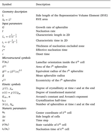
Table 1
List of symbols.
Symbol Description
Geometry description
L Side length of the Representative Volume Element (RVE)
=
S0 L2 RVE area Input parameters
G Growth rate of spherulite
I Nucleation rate
=
Lc G I13 13 Characteristic length in 2D
=
tc G I23 13 Characteristic time in 2D
Ld Thickness of nucleation excluded zone
t Effective nucleation time
τ Onset time
Microstructural symbols
x
( )k Lamellar orientation inside the kthcell
S( )i Area of the ithspherulite
=
R( )i (S( )i/ )0.5 Equivalent radius of the ithspherulite
R Mean spherulite radius
e( )i Eccentricity of the ithspherulite
Kinetic symbols t
( ), Degree of crystallinity at time t and at the end
=
t t
( ) ( )/ Degree of transformed material
KAv, n Avrami's constant and Avrami's exponent
t0.5 Crystallization half-time
N t( ), N Number of spherulites at time t and at the end
Numeric paramaters
xk Center coordinate of kthcell
x Side length of cells
t Time step
x
( )k State variable of kthcell
2.1. Concept of nucleation time
We propose to model the spherulite nucleation for isothermal crystallization with the concept of nucleation time, t x0( )k. The
nuclea-tion time, t x0( )k, is a random time associated with the kthcell of
co-ordinates xk. It defines the onset time of the first germ for kthcell. It is
randomly generated (seeFig. 3(a)) at the beginning of each simulation by the following expression:
= + =
t0( )xk ( )xkt0max , with rand(0,1), (1)
where τ is the onset time andtmax=I ( x)
0 1 2is the time where the
nucleation is certain inside the cell of surface x( )2 for a given
nu-cleation rate, I.
To model the nucleation saturation, two different ideas are studied (see Fig. 3). Firstly, we propose to introduce an effective nucleation time,t <tmax
0 , which acts as a superior limit of the nucleation time
(seeFig. 3(a)), such as:
= + > t x x t x x ( ) ( ) if ( ) if ( ) k k max k max k max 0 0 (2) where0 ( )xk <1is a random field and max= t t/0max.
Secondly, we also study an excluded nucleation zone around spherulites [23], modeled by a length parameterLd, which is the layer
thickness where the nucleation is inhibited (seeFig. 3(b)).
The effective nucleation time controls the spherulite number (cf.
Equation(13)), this concept could be used to model the effect of
nu-cleating agents. The existence of an excluded nucleation zone may be due to thermo-mechanical or diffusional effects around the spherulite that would promote growth over nucleation, such as the depletion zone observed in thin films [8]. Note that it is possible to model the nu-cleation using the activation frequency and the saturation by introdu-cing the nucleus density [31,32,76,77].
2.2. Algorithm of growth and nucleation
The pixel coloring algorithm [31,32,76,77] is used to model the spherulite growth. In this method, we take advantage of isotropic growth of spherulites at the microscale for isothermal crystallization. The transformation rule describing the phase change (seeFig. 4) is as follows: if the molten cell xk, i.e. ( )xk =0, is inside theithcircle, so the
cell is transformed intoith spherulite, ( )x = i
k . Theith circle, which
represents the shape of the spherulite if it is isolated from other spherulites, is defined by its radiusR( )i ( )t =G t( ti)
0( ) , where t0( )i is the
nucleation time associated with theithspherulite andxi 0
( ), its nucleation
point. Note that periodic boundary conditions (seeFig. 4) are applied to avoid edge effects. The simulation algorithm is as follows:
1. Random generation of nucleation time t x0( )k for all cells
2. Time loop fort {0; t; 2 ; ;t…N t}
(a) Nucleation step: Creation of a new ith spherulite of center,
= xi x
k
( ) ift x( )<t k
0 and the cell ofxk is inside the melt area
where the nucleation is possible. (b) Growth step: Loop over allithspherulites
•
ComputeR( )i ( )t =G t( ti)0( )
•
Transform the molten cells inside theithcircle associated withtheithspherulite
3. Post-processing
2.3. Post-processing
At the end of the simulation, all the cells have been assigned to one spherulite. We obtain the final morphology of the spherulite micro-structure. We compute two types of information, which are linked to the microstructure and the kinetics. These data are then used to perform our statistical analyses.
2.3.1. Microstructural analysis
The area S( )i of the spherulite i can be obtained by collecting its
cells, from which we can directly calculate the equivalent radius of the spherulite, such as:
= R( )i S( )i .
(3)
The mean value,R is estimated from several simulations.
The growth direction of crystalline lamellae is assumed radial (see
Fig. 2). We define the lamella orientation, x( )k, as the angle between
the lamella growth direction given by the vector x( k( )i x i)
0( ) and the
x-axis for allxk( )i inside theithspherulite.
Fig. 2. Representative volume element of the spherulite modeling, where xi
0 ( )is
the nucleation center of spherulite i and x( )k the lamella orientation at point
xk.
Fig. 3. Scheme of the two strategies to model the nucleation saturation: (a)
Introduction of effective nucleation time t ; (b) Introduction of the excluded nucleation zone Ld[23].
Fig. 4. Schematic representation of the growth step used under periodic
2.3.2. Kinetic analysis
During the simulation, the number of spherulites, N t(), and the degree of transformed material, ( )t are stored at each step time. The degree of transformed material is given by:
= t n t n ( ) 1 ( ) t 0 (4) wheren t0( )is the number of molten cells at time t andnt the total
number of cells in the simulation box. For isothermal cases, the degree of transformed material is related to the degree of crystallinity, such as
=
t t T
( ) ( )/ ( )where ( )T is the final degree of crystallinity at the
given temperature T.
The Avrami theory is applied to analyze the isothermal crystal-lization kinetics by fitting the data with the following equation:
=
t K t
( ) 1 exp( ( Av ) )n (5)
where Avrami's parameters are the exponent n and the Avrami's char-acteristic timeKAv. The exponent n are determined by linear regression
of Avrami's plot with ( )t in the range from 0.05 to 0.95. The Avrami's characteristic timeKAvis determined by measuring the crystallization
half-timet0.5=(ln 2)KAvn
1
.
2.4. Model parameters
There are four parameters that control the crystallization model growth: the nucleation rate, I, the growth rate G, the effective nuclea-tion time, t , and the thickness of nucleanuclea-tion exclusion zone,Ld. In our
study, we introduce two new parameters instead of G and I: a char-acteristic length,Lc, and a characteristic time, tc(seeTable 2), defined
by: = + = + L G I , t (G I) c d c d d 1 1 1 1 (6)
where =d 2 is the dimension of space. According to the isothermal
crystallization properties of various semi-crystalline polymers at dif-ferent crystallization temperature [11], the characteristic length, Lc,
ranges from 10 to102μm and the characteristic time, tc, ranges from
10 3to 105s. As we will see in Section3, the parametersL
cand tccontrol
the size of the microstructure and the kinetics, respectively. It will be shown that the final average spherulite diameter isLc2and that tcis the
time over which nuclei are formed without considering nucleation sa-turation.
In addition to the parameters of the model, we have the parameters related to the simulation: the size of the simulation box, L; the space
step, x and the time step, t. The space step is chosen at x=1μm
which is of the same order of magnitude as the resolution of an optical microscope. The time step is chosen to guarantee the proper functioning of the algorithm such as t=min(G x/3,t0.5/50).
3. Simulation results
This section presents 2D simulation results of the morphology and the kinetics of the spherulite growth. The influence of four parameters,
i.e.Lc, tc, L Ld/ cand t t/c, are analyzed in details. We use the additional
parameters L Ld/ cand t t/cbecause they control the effect of nucleation
saturation independently of the values ofLc and tc. Each simulation is
based on the square RVE of =L 500μm, and500×500cells with length
=
x 1μm are employed. Besides, the onset time is fixed as = 0 s. 3.1. Spherulitic morphology
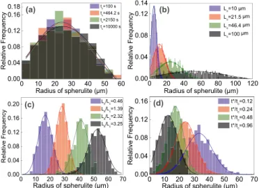
The influence of the four parameters on the spherulitic morphology is depicted inFig. 5. In each row, three of the four parameters are fixed, and the evolution of spherulitic microstructure along with the increase of the remaining parameter can be observed.Fig. 6(a–d) represents the spherulite size distribution at the final stage of crystallization in terms
Table 2
Model parameters.
Variable Description Space Lc=G I1/3 1/3 Characteristic length
variables Ld Thickness of excluded nucleation zone
Time tc=G2/3I 1/3 Characteristic time
variables t Effective nucleation time
Fig. 5. Examples of final spherulitic morphologies at various cases. The color
contrast is due to the lamellar orientation, θ, inside the spherulites. (All results are presented using Paraview software [106]). (For interpretation of the re-ferences to color in this figure legend, the reader is referred to the Web version of this article.)
Fig. 6. Simulated spherulite size distributions in terms of spherulite radius. The
lines represent curve fits by the use of normal distribution. (a)Lc=46.4μm,
=
L Ld/ c 0, and =t t0max; (b) =tc 2150s,L Ld/ c=0, and =t t0max; (c) =t t0max, =
Lc 21.5 μm, and tc=2.15×10³ s; (d) L Ld/ c=0, Lc=21.5 μm, and
= ×
of the spherulite radius for the various cases corresponding to
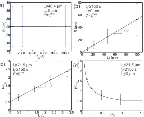
Fig. 5(a–d). The results are fitted by using a normal distribution. Fi-nally,Fig. 7gives the spherulite radius and its standard deviation versus the four parameters.
Firstly, tc is increased from 100 s to104 s by fixingLc=46.4 μm,
=
Ld 0, andt =t0max. The change of tcwhile keepingLcas a constant is
obtained by adapting G and I according to Eq.(6). The value ofLc is
fixed at higher value to obtain larger spherulites which are easier to
observe and the other two parameters are fixed at Ld=0 μm, and
= t tmax
0 to avoid the influence of the nucleation saturation. The
spherulitic microstructures are shown inFig. 5(a), where it is obvious that the size of spherulite does not change with tc.Fig. 6(a) shows the
spherulite size distribution at the final stage of crystallization in terms of the spherulite radius over the range of provided tc, indicating
ap-proximately the same average value and distribution. It can also be seen in Fig. 7(a) that the mean radius and the standard deviation keeps constant at various tc, which further confirmed the independence of the
spherulite size with tc.
In order to study the influence ofLc, we set =tc 2150s,Ld=0μm,
andt =tmax
0 (to avoid the influence of nucleation saturation), and we
increasedLc from 10 μm to 100 μm. The corresponding morphologies
are shown inFig. 5(b), demonstrating that the number of spherulites
decreases along with increasing Lc, while the size of the spherulites
raises.Fig. 6(b) shows the spherulite size distribution at the final stage of crystallization in terms of the spherulite radius over the range of providedLc. It can be observed that the final spherulite size shifts
tre-mendously to higher values from the condition of smallLcwith a large
number of nuclei to the condition of largeLc with a small number of
nuclei. Furthermore, we summarized the radius of spherulites for the four conditions. The results are plotted as a function ofLcinFig. 7(b),
where the mean radius and its standard deviation are presented. It is very interesting to see the mean radius obey a linear increase along
withLc with a tangent of 0.53, and the standard deviation grows
si-multaneously. As we expected, the characteristic length,Lc, is close to
the equivalent diameter of the spherulite. Therefore, we can find that the mean spherulite radius,R, is roughly equal to0.5Lc.
The nucleation exclusion zone also has a tremendous effect on the
morphology in the numerical model, whose length is introduced byLd.
Thus, we sett =tmax
0 to neglect the effect of end time of nucleation,
=
Lc 21.5μm, and =tc 2.15×10³s, and the non-dimensional parameter L Ld/ cratio is increased from 0.46 to 3.25 with a step of 0.92 which is
associated with the length of nucleation exclusion zoneLdranging from
10 μm to 70 μm with a step of 20 μm.Fig. 5 (c) presents the
corre-sponding morphologies at various L Ld/ c, where the increase of
spher-ulite size can be observed.Fig. 6(c) gives the simulated spherulite size distributions in terms of the spherulite radii over the range of in-vestigated L Ld/ cvalues. The size of spherulites presents a gradual shift
to larger values from low L Ld/ c to high L Ld/ cratio, resulting from the
decreasing number of nuclei. Moreover, the spherulite radii R are cal-culated for the four cases respectively, and we plot R L/ c and its
stan-dard deviation as a function of L Ld/ c ratio, as shown inFig. 7(c). It is
shown that the mean value of R L/ c increases linearly along with the
L Ld/ cratio, but the standard deviation remains unchanged. It should be
pointed out that the tangent of the curve is independent onLcand tc.
Finally, the effect of effective nucleation time t on the morphology in the numerical model is studied. We setL Ld/ c=0to neglect the effect of the nucleation exclusion zone,Lc=21.5μm, and =tc 2.15×10³s,
and the non-dimensional parameter t t/cratio, which is associated with
the end time of nucleation, is increased from 0.12 to 0.96, produces the
corresponding final morphology as presented inFig. 5(d).Fig. 6(d)
gives the simulated spherulite size distributions in terms of the spher-ulite radii over the range of investigated t t/cvalues, where the size of
spherulites presents a gradual shift to lower values from small t t/cto
large t t/c, resulting from the increasing number of nuclei. Then, the R L/ cratio and its standard deviation related to spherulite radius R are
plotted for the four cases respectively, showing a decrease in the averaged value along with t t/c. It should be pointed out that the
tan-gent of the curve is independent onLc and tc. However, the standard
deviation of the spherulite size does not seem to be influenced by t t/c. 3.2. Kinetic properties
Fig. 8 presents the Avrami analysis for the cases with various combination of parameters, where the first column is the Avrami plot
and the second column indicates the Avrami parameter n and crystal-lization half-time t0.5versus the varying parameters, according to the
conditions set inFig. 5. Each curve of the Avrami plot is obtained as an average of 10 random samples. Moreover, the normalized spherulite density, NL Lc2/ 2, as a function of normalized time,t t/c, is plotted in
Fig. 9 for the corresponding cases, where we can see the normalized spherulite density increases until reaching a plateau. N denotes the number of spherulites. Each curve is calculated by taking the average value of 10 random samples, and the colored region represents the interval of these samples.
Firstly, we setLc=46.4μm,Ld=0μm, and =t* t0max, and increased tc from 100 s to104s. The Avrami plots are shown on the left inFig. 8
(a). The crystallization half-time, t0.5 and the Avrami exponent, n are
plotted as a function of tc for the four cases correspondingly on the
right. It can be seen that n is constant which is in good agreement with
the theoretical value =n 3for the 2D uniform nucleation and growth,
and t0.5increases linearly along with tc. Moreover, the spherulite density
as a function of crystallization time is plotted inFig. 9(a). FixingLc, we
can find that the nucleation rate decreases with increasing tc, but the
spherulite density finally reaches the same level.
Then, at fixed =tc 2150s,Ld=0μm, and =t* t0max,Lcwas increased
from 10 μm to 100 μm. InFig. 8(b), it is noteworthy that n and t0.5
remain constant, showing that the crystallization rate is independent of
Lc.Fig. 9(b) presents the spherulite density versus crystallization time
for the corresponding four cases, where the curves reach a plateau at the same time.
The Avrami analysis on the kinetic characteristics under various
L Ld/ cratio is given on the left inFig. 8(c) by fixing =t* t0max,Lc=21.5
Fig. 8. Kinetic analysis for the various cases. The first column denotes Avrami plots for the isothermal crystallization of the corresponding conditions, and the second
μm, and =tc 2.15×10³s. The corresponding Avrami exponent n and crystallization half-time t0.5as a function of L Ld/ care shown on the right
inFig. 8(c). It can be seen that n decreases from 3.0 to 2.3 for the four increasing L Ld/ c cases. The crystallization half-time t0.5grows with
in-creasing L Ld/ cratio, indicating a decrease in the kinetics. Besides, the
number of spherulites versus crystallization time is provided inFig. 9
(c). It is obvious that the number of spherulites grows linearly at the initial time with the same nucleation rate, and finally reaches a plateau, which goes up with decreasing L Ld/ c. It indicates that the higher L Ld/ c
leads to less nuclei resulting from the large nucleation exclusion zone. Finally, the Avrami analysis on the kinetic characteristics under various t t/* cratio is presented on the left inFig. 8(d) whenL Ld/ c=0,
=
Lc 21.5μm, and =tc 2.15×10³s. The corresponding Avrami exponent n and crystallization half-time t0.5 as a function of t t/* c ratio are also
given. It can be seen that n increases from 2.1 to 3.0 for the four in-creasing t t/* ccases. The crystallization half-time t0.5falls with increasing t t*/c ratio, indicating an acceleration in the kinetics. Besides, the
spherulite density versus crystallization time is provided inFig. 9(d), which indicates that the higher t t/* c ratio leads to more nuclei due to
the larger nucleation time. 4. Further discussion
4.1. Parameter influence
4.1.1. Influence of the characteristic lengthLcand the characteristic time tc
First of all, we note that the microstructure and the crystallization rate depend jointly on the nucleation rate, I, and the growth rate, G. More precisely, the average spherulite area (respectively the number of spherulites, N) is proportional to the square of the characteristic length
=
Lc G I1/3 1/3(respectively N 1/Lc2), whereasLchas no effect on the
kinetics of crystallization. The characteristic time, =tc G 2/3I 1/3,
con-versely, controls the kinetics and has no influence on the final mor-phology. In the case where the nucleation saturation is not considered, the normalized density of spherulites (NL Lc2/ 2) versus the normalized
time (t t/c) curve is universal whatever the values of I and G
(Fig. 9(a–b)). We obtain a master curve with an initial slope equal to 1, which saturates for >t 1.4tcat 0.85. This means that the nucleation rate
in our simulation is indeed =I 1/(t Lc c2)and that the average maximum number of spherulites inside a surfaceS0=L2is equal to0.85 /S L0 c2.
The two parameters, t andLd, are useful to model the nucleation
saturation before the crystallization ends (seeFig. 9(c–d)). Both have an influence on the kinetics and the microstructure.
4.1.2. Influence of the effective nucleation time, t
At first, we discuss the influence of the effective nucleation time, t . For this discussion, it is useful to recall and transpose the Avrami Evans Kolmogorov Johnson Mehl type model. Following the review of Piorkowska and Haudin [107], the degree of transformed material, ( )t
is defined by: = t E t S ( ) 1 exp ( ) 0 (7)
whereE t( )is the ‘extended surface’ which is equal to the total surface of all domains growing from all nuclei inside the reference surface, without considering the impingement of growing domains. It is defined in 2 dimensions by: = E t( ) t G t( u) d ( )N u 0 2 2 (8) whered ( )N u is the number of nuclei created at time u insideS0. Here,
we assume thatd ( )N u is proportional to both the nucleation rate, I, and the reference surface,S0, for <t t , so that:
= < N u S I u u t u t d ( ) d 0 0 (9) After integration, we obtain:
= = < = +
( )
E t S IG t u u S t t S IG t u u S t tt t t t ( ) ( ) d for ( ) d (3 3 ( ) ) for t t t t t t 0 0 2 2 3 0 3 0 0 2 2 3 0 2 2 c c3 (10)Below t , this model is similar to the Avrami model with an
ex-ponent =n 3, above t , the behavior tends to a model of Avrami with
an exponent =n 2. It is interesting to note that for sporadic nucleation
without nucleation saturation (t and L Ld/ c=0), this model
predicts an exponent n=3 and the crystallization half-time
=
(
)
t0.5 3ln 2 tc 0.90tc 1
3 . These values are obtained by numerical
si-mulation (seeFig. 8a). The asymptotic approximation of equation(10)
suggests the following relationship between n and the ratio t t/c: > < n 3 0.99 0.09 0.99 2 0.09 t t t t t t 14.2 4.72 ln c t tc c c (11)
Note that the simulation results and this equation provide the range of t in which the nucleation is purely sporadic ( =n 3) or instantaneous
( =n 2) according to Avrami's approach. The asymptotic approximation
suggests also the relationship between t t/0.5 c and t t/c: > + <
( )
( )
t t 0.90 0.49 0.37 1 0.07 0.49 0.47 0.07 c t t t t t t t t t t 0.5 c c c c c 1 2 1 2 (12) The parameter of these relationships are fitted on the simulation results, except for the law given for t t/0.5 c at very small values of<
t t/c 0.07. In fact, the ‘extended surface’ is given by the first order approximation of Equation(10), E t( ) S t t t t0( / )( / )c c 2, for very small
value of t t/c<0.07. For this case, we have
=
t0.5/tc (ln(2)/ ) ( / )12 t tc 21 0.47( / )t tc 12.
From the microstructural point of view, Equation(9)gives the final number of spherulites,N inside the reference surfaceS0:
= = = N N t S It S L t t ( ) c c 0 02 (13)
So, the mean value of spherulite area, S is given by
= =
S N S/ 0 L t tc c2 / . Assuming thatS is proportional to R2, we obtain the following expression:
>
( )
R L 0.53 1 0.53 1 c t t t t t t c c c 1 2 (14) Here, the parameters are fitted from the simulation results. A goodagreement is observed with the simulation results (seeFigs. 7(d) and
8(d)).
4.1.2. Influence of the thickness of the nucleation excluded zoneLd
The simulation results suggest that the following relationship for the mean radius is (seeFig. 7(c)):
+ R L L L 0.57 0.9 c d c (15)
From the kinetic point of view, the comparison with Avrami's type model would require the introduction of the nucleation excluded zone concept. This would be possible but it is outside the scope of the present paper as it needs specific numerical methods to solve this kind of pro-blem. Here, we prefer to proceed by analogy by taking inspiration from the simulation results. Indeed, all the kinetic and microstructural parameters vary linearly with the ratio t t( / )c 12(see Equations(11), (12) and (14)). We also find that these parameters vary linearly with the
L Ld/ cratio. This is why we propose the following relationship to fit the
simulation data: < > + n 3 1.12 1.12 6.05 2 6.05 L L L L L L 10.1 ln 3.25 d c Ld Lc d c d c (16) + > t t 0.90 0.69 0.36 0.65 0.69 c L L L L L L 0.5 d c d c d c (17)
Here, these relationships are fitted from simulation results. A good
agreement is observed with the simulation results (seeFigs. 7(c) and
8(c)).
4.2. Comparison between the two modeling hypotheses of the nucleation saturation
Two assumptions have been studied in this paper to model the nucleation saturation: the excluded nucleation zone, which is defined by the thicknessLd, and the effective nucleation time, t . Although both
hypotheses induce changes in the Avrami exponent, n, from 2 to 3, they exhibit significantly different effects on the crystallization half-time,
t0.5, and the spherulite mean radius,R.
For the kinetics, we can see the difference by looking at the evo-lution of the normalized spherulite density as a function of normalized
time (see Fig. 9(c–d)). The transition between the part, where the
density increases proportionally with time, and the plateau is smoother for the excluded nucleation zone assumption (Fig. 9(c)).
Furthermore, in case of the excluded nucleation zone assumption, the size distributions of spherulite radii show no spherulite of radius less thanLd(seeFig. 6(c–d)). This assumption also changes the relative
position of the nucleus inside the spherulite. We introduce the eccen-tricity of theithspherulite,e
i to study this effect (Fig. 10(a)). It is
de-fined by =ei d Ri/ ( )i; where =di x0( )i xg( )i is the distance between the
spherulite nucleus,x i
0( ), and its centroidxg( )i. The value of e is presented
as a function of the Avrami exponent n inFig. 10(b). The average
ec-centricity does not seem affected by the effective nucleation time, whereas the existence of the excluded nucleation zone halves its value. It is noteworthy that for low L Ld/ c that do not affect the kinetics
( =n 3), there is a significant effect on the average eccentricity. This effect is explained by the fact that the nucleus cannot be at a distance less thanLdfrom the spherulite boundary.
We believe that the experimental study of the eccentricity of spherulites will make it possible to choose or discriminate against one or the other assumptions used to model nucleation staturation, i.e. istence of an effective nucleation time or existence of a nucleation ex-cluded zone. Specifically, at a certain Avrami parameter n, if the ec-centricity of the spherulites is obvious, the effective nucleation time assumption algorithm can be employed in the modeling. Otherwise, we rather choose the nucleation excluded zone assumption algorithm.
4.3. Relationships between kinetics and microstructure
The last interesting point is the relationship between kinetics and microstructure. Indeed, if we know the growth rate, G, it is possible to generate an equivalent microstructure from the results of the Avrami analysis. More precisely, the Avrami exponent, n, and the crystal-lization half-time, t0.5, provide us the value of tcand t (orLd) as shown
in Steps 1 and 2 of the previous subsection. Finally, the characteristic length is given byLc=Gtc. It is interesting to note that this approach
allows to compute the nucleation rate, =I L tc2c1, from the Avrami
parameters and the growth rate G by the following expression:
= + I G t n 0.051 1 exp 7.10 2.36 2 0.53 3 (18)
this expression is valid for 2D cases and for < n2 3. It should be noted that the surface effects which can lead to transcrystallinity are not taken into account.
Note that Billon and Haudin [108] also provided an algorithm to
determine the nucleation rate, I, by combining the isothermal crystal-lization experiments with the computational simulation.
5. Conclusions
The numerical framework, which is presented in this paper, allows to generate 2D microstructures of isothermal crystallization from phy-sical data such as growth rate, G, and nucleation rate, I. The new concept of nucleation time can well impose the sporadic nucleation or predetermined nucleation (instantaneous nucleation) by introducing the effect of nucleation saturation. Two assumptions have been studied to model the nucleation saturation, namely the existence of an effective nucleation time, t , or the existence of a nucleation excluded zone of thickness,Ld.
An analysis was carried out using the characteristic length,
= Lc G I
1
3 13, and the characteristic time, =tc G I23 13, as well as two
adimensional parameters (t t/c and L Ld/ c) associated with the two
previous assumptions, leading us to the following remarks:
•
The mean spherulite radius,Ris proportional toLcand independentof tc; with a proportionality constant that depends on the
di-mensionless numbers t t/cand L Ld/ c (cf. Equations(14) and (15)).
•
Conversely, the crystallization half-time, t0.5is proportional to tcandindependent ofLc; with a proportionality constant that depends on
the dimensionless numbers t t/cand L Ld/ c (cf. Equations(12) and
(17)).
•
The nucleation saturation influences the Avrami exponent, n, (cf.Equations 11 and 16), which varies continuously from 3 (no
sa-turation) to 2 (high sasa-turation) for both studied assumptions. In addition, the saturation of the nucleation increases the mean radius of the spherulites and the crystallization half-time according to the
laws given by Equations(12) and (14)using the assumption of the
existence of an effective nucleation time, and by Equations(15) and (17)using the assumption of the existence of a nucleation excluded zone.
•
These simulations allow to highlight a relationship betweencrys-tallization kinetics and microstructure. These results suggest that it is possible to generate a microstructure from data from a DSC iso-thermal analysis, provided that the growth rate G is known (cf. Equation(18)). Nevertheless, a 3D crystallization occurs during DSC experiment. This is the reason why it is necessary to have a 3D numerical framework.
It is interesting to note that the efficiency of our numerical frame-work offers the possibility to perform 3D simulations containing several hundred spherulites. The extension to 3D cases will be the subject of a further publication [109].
Aknowledgements
The authors thank the financial support of the F2M (Fédération francilienne de mécanique, Coup de pouce 2017).
References
[1] C. Thomas, R. Seguela, F. Detrez, V. Miri, C. Vanmansart, Plastic deformation of spherulitic semi-crystalline polymers: an in situ AFM study of polybutene under tensile drawing, Polymer 50 (15) (2009) 3714–3723.
[2] F. Detrez, S. Cantournet, R. Seguela, Plasticity/damage coupling in semi-crystal-line polymers prior to yielding: micromechanisms and damage law identification, Polymer 52 (9) (2011) 1998–2008.
[3] A. Pawlak, A. Galeski, A. Rozanski, Cavitation during deformation of semi-crystalline polymers, Prog. Polym. Sci. 39 (5) (2014) 921–958.
[4] N. Selles, P. Cloetens, H. Proudhon, T.F. Morgeneyer, O. Klinkova, N. Saintier, L. Laiarinandrasana, Voiding mechanisms in deformed polyamide 6 observed at the nanometric scale, Macromolecules 50 (11) (2017) 4372–4383.
[5] M. Raimo, “Kinematic” analysis of growth and coalescence of spherulites for predictions on spherulitic morphology and on the crystallization mechanism, Prog. Polym. Sci. 32 (6) (2007) 597–622.
[6] R. Castillo, A. Müller, Crystallization and morphology of biodegradable or bio-stable single and double crystalline block copolymers, Prog. Polym. Sci. 34 (6) (2009) 516–560.
[7] E. Piorkowska, G.C. Rutledge (Eds.), Handbook of Polymer Crystallization, John Wiley & Sons, 2013.
[8] R.E. Prud’homme, Crystallization and morphology of ultrathin films of homo-polymers and polymer blends, Prog. Polym. Sci. 54 (2016) 214–231.
[9] B. Crist, J.M. Schultz, Polymer spherulites: a critical review, Prog. Polym. Sci. 56 (2016) 1–63.
[10] K.N. Okada, M. Hikosaka, Handbook of Polymer Crystallization, John Wiley & Sons, 2013, pp. 125–163 Ch. Polymer Nucleation.
[11] N. Okui, S. Umemoto, R. Kawano, A. Mamun, Temperature and molecular weight dependencies of polymer crystallization, Progress in Understanding of Polymer Crystallization, Springer, 2007, pp. 391–425.
[12] A. Gałeski, Z. Bartczak, M. Pracella, Spherulite nucleation in polypropylene blends with low density polyethylene, Polymer 25 (9) (1984) 1323–1326.
[13] P. McGenity, J. Hooper, C. Paynter, A. Riley, C. Nutbeem, N. Elton, J. Adams, Nucleation and crystallization of polypropylene by mineral fillers: relationship to impact strength, Polymer 33 (24) (1992) 5215–5224.
[14] P.-D. Hong, W.-T. Chung, C.-F. Hsu, Crystallization kinetics and morphology of poly (trimethylene terephthalate), Polymer 43 (11) (2002) 3335–3343. [15] I. Coccorullo, R. Pantani, G. Titomanlio, Crystallization kinetics and solidified
structure in ipp under high cooling rates, Polymer 44 (1) (2003) 307–318. [16] N.-y. Ning, Q.-j. Yin, F. Luo, Q. Zhang, R. Du, Q. Fu, Crystallization behavior and
mechanical properties of polypropylene/halloysite composites, Polymer 48 (25) (2007) 7374–7384.
[17] A.T. Lorenzo, M.L. Arnal, J. Albuerne, A.J. Müller, DSC isothermal polymer crystallization kinetics measurements and the use of the Avrami equation to fit the data: guidelines to avoid common problems, Polym. Test. 26 (2) (2007) 222–231. [18] M. Abolhasani, A. Jalali-Arani, H. Nazockdast, Q. Guo, Poly (vinylidene fluoride)-acrylic rubber partially miscible blends: crystallization within conjugated phases Fig. 10. a) Schematic representation of the algorithm used to generate the microstructure under periodic boundary conditions. b) e versus Avrami parameter n for the
two algorithms which introduce nucleation saturation.Lc=21.5μm, =tc 2.15×10³s. The red curve denotes the effective nucleation time algorithm, and the blue
curve denotes the nucleation excluded zone algorithm. (For interpretation of the references to color in this figure legend, the reader is referred to the Web version of this article.)
induce dual lamellar crystalline structure, Polymer 54 (17) (2013) 4686–4701. [19] H. Takeshita, T. Shiomi, K. Takenaka, F. Arai, Crystallization and higher-order
structure of multicomponent polymeric systems, Polymer 54 (18) (2013) 4776–4789.
[20] S. Gupta, X. Yuan, T.M. Chung, M. Cakmak, R. Weiss, Isothermal and non-iso-thermal crystallization kinetics of hydroxyl-functionalized polypropylene, Polymer 55 (3) (2014) 924–935.
[21] L. Jin, J. Ball, T. Bremner, H.-J. Sue, Crystallization behavior and morphological characterization of poly (ether ether ketone), Polymer 55 (20) (2014) 5255–5265. [22] J.Y. Lim, J. Kim, S. Kim, S. Kwak, Y. Lee, Y. Seo, Nonisothermal crystallization
behaviors of nanocomposites of poly (vinylidene fluoride) and multiwalled carbon nanotubes, Polymer 62 (2015) 11–18.
[23] I.V. Markov, Crystal growth for beginners: fundamentals of nucleation, crystal growth and epitaxy, World Sci. (2016) 130.
[24] E. Koscher, R. Fulchiron, Influence of shear on polypropylene crystallization: morphology development and kinetics, Polymer 43 (25) (2002) 6931–6942. [25] R.I. Tanner, F. Qi, A comparison of some models for describing polymer
crystal-lization at low deformation rates, J. Non-Newtonian Fluid Mech. 127 (2–3) (2005) 131–141.
[26] T.B. van Erp, L. Balzano, A.B. Spoelstra, L.E. Govaert, G.W.M. Peters, Quantification of non-isothermal, multi-phase crystallization of isotactic poly-propylene: the influence of shear and pressure, Polymer 53 (25) (2012) 5896–5908.
[27] M. van Drongelen, P.C. Roozemond, G.W.M. Peters, Non-isothermal crystallization of semi-crystalline polymers: the influence of cooling rate and pressure, Adv. Polym. Sci. 277 (2017) 207–242.
[28] M. van Drongelen, T.B. Van Erp, G.W.M. Peters, Quantification of non-isothermal, multi-phase crystallization of isotactic polypropylene: the influence of cooling rate and pressure, Polymer 53 (21) (2012) 4758–4769.
[29] E. Piorkowska, Modeling of polymer crystallization in a temperature gradient, J. Appl. Polym. Sci. 86 (6) (2002) 1351–1362.
[30] J.-M. Escleine, B. Monasse, E. Wey, J.-M. Haudin, Influence of specimen thickness on isothermal crystallization kinetics. A theoretical analysis, Colloid Polym. Sci. 262 (5) (1984) 366–373.
[31] N. Billon, J.-M. Haudin, Overall crystallization kinetics of thin polymer films. General theoretical approach. I Volume nucleation, Colloid Polym. Sci. 267 (12) (1989) 1064–1076.
[32] N. Billon, J.-M. Escleine, J.-M. Haudin, Isothermal crystallization kinetics in a limited volume. A geometrical approach based on Evans' theory, Colloid Polym. Sci. 267 (8) (1989) 668–680.
[33] N. Billon, C. Magnet, J.-M. Haudin, D. Lefebvre, Transcrystallinity effects in thin polymer films. Experimental and theoretical approach, Colloid Polym. Sci. 272 (6) (1994) 633–654.
[34] T. Choupin, B. Fayolle, G. Regnier, C. Paris, J. Cinquin, B. Brulé, Isothermal crystallization kinetic modeling of poly (etherketoneketone)(PEKK) copolymer, Polymer 111 (2017) 73–82.
[35] T. Choupin, B. Fayolle, G. Régnier, C. Paris, J. Cinquin, B. Brulé, A more reliable dsc-based methodology to study crystallization kinetics: application to poly (ether ketone ketone)(PEKK) copolymers, Polymer 155 (2018) 109–115.
[36] M. Avrami, Kinetics of phase change. I General theory, J. Chem. Phys. 7 (12) (1939) 1103–1112.
[37] M. Avrami, Kinetics of phase change. II Transformation-time relations for random distribution of nuclei, J. Chem. Phys. 8 (2) (1940) 212–224.
[38] M. Avrami, Kinetics of phase change. III: granulation, phase change and micro-structure, J. Chem. Phys. 9 (1941) 177–184.
[39] U.R. Evans, The laws of expanding circles and spheres in relation to the lateral growth of surface films and the grain-size of metals, Trans. Faraday Soc. 41 (1945) 365–374.
[40] T. Ozawa, Kinetics of non-isothermal crystallization, Polymer 12 (3) (1971) 150–158.
[41] K. Nakamura, T. Watanabe, K. Katayama, T. Amano, Some aspects of non-isothermal crystallization of polymers. i. relationship between crystallization temperature, crystallinity, and cooling conditions, J. Appl. Polym. Sci. 16 (5) (1972) 1077–1091.
[42] K. Nakamura, K. Katayama, T. Amano, Some aspects of nonisothermal crystal-lization of polymers. II consideration of the isokinetic condition, J. Appl. Polym. Sci. 17 (4) (1973) 1031–1041.
[43] E. Piorkowska, N. Billon, J.-M. Haudin, J. Kolasinska, Spherulitic structure de-velopment during crystallization in a finite volume, J. Appl. Polym. Sci. 86 (6) (2002) 1373–1385.
[44] E. Piorkowska, N. Billon, J.-M. Haudin, K. Gadzinowska, Spherulitic structure development during crystallization in confined space II. Effect of spherulite nu-cleation at borders, J. Appl. Polym. Sci. 97 (6) (2005) 2319–2329.
[45] Y. Yuryev, P. Wood-Adams, A Monte Carlo simulation of homogeneous crystal-lization in confined spaces: effect of crystalcrystal-lization kinetics on the Avrami ex-ponent, Macromol. Theory Simul. 19 (5) (2010) 278–287.
[46] Y. Yuryev, P. Wood-Adams, Effect of surface nucleation on isothermal crystal-lization kinetics: theory, simulation and experiment, Polymer 52 (3) (2011) 708–717.
[47] W. Hu, D. Frenkel, V.B. Mathot, Simulation of shish-kebab crystallite induced by a single prealigned macromolecule, Macromolecules 35 (19) (2002) 7172–7174. [48] M. Muthukumar, Modeling polymer crystallization, Adv. Polym. Sci. 191 (2005)
241–274.
[49] T. Yamamoto, Molecular dynamics modeling of the crystal-melt interfaces and the growth of chain folded lamellae, Adv. Polym. Sci. 191 (2005) 37–85. [50] R.H. Gee, L.E. Fried, Atomistic simulation of polymer crystallization at realistic
length scales, Nat. Mater. 5 (2006) 39–43.
[51] J. Zhang, M. Muthukumar, Monte Carlo simulations of single crystals from polymer solutions, J. Chem. Phys. 126 (23) (2007) 234904.
[52] S. Cheng, W. Hu, Y. Ma, S. Yan, Epitaxial polymer crystal growth influenced by partial melting of the fiber in the single-polymer composites, Polymer 48 (14) (2007) 4264–4270.
[53] T. Yamamoto, Computer modeling of polymer crystallization–toward computer-assisted materials' design, Polymer 50 (9) (2009) 1975–1985.
[54] Y. Ren, L. Zha, Y. Ma, B. Hong, F. Qiu, W. Hu, Polymer semicrystalline texture made by interplay of crystal growth, Polymer 50 (25) (2009) 5871–5875. [55] C. Baig, B.J. Edwards, Atomistic simulation of crystallization of a polyethylene
melt in steady uniaxial extension, J. Non-Newtonian Fluid Mech. 165 (17–18) (2010) 992–1004.
[56] N. Waheed, M. Ko, G. Rutledge, Molecular simulation of crystal growth in long alkanes, Polymer 46 (20) (2005) 8689–8702.
[57] G.C. Rutledge, Handbook of Polymer Crystallization, John Wiley & Sons, 2013, pp. 197–214 Ch. Computer Modeling of Polymer Crystallization.
[58] Y. Nie, H. Gao, M. Yu, Z. Hu, G. Reiter, W. Hu, Competition of crystal nucleation to fabricate the oriented semi-crystalline polymers, Polymer 54 (13) (2013) 3402–3407.
[59] Y. Nie, R. Zhang, K. Zheng, Z. Zhou, Nucleation details of nanohybrid shish-kebabs in polymer solutions studied by molecular simulations, Polymer 76 (2015) 1–7. [60] A. Ziabicki, Generalized theory of nucleation kinetics. I. General formulations, J.
Chem. Phys. 48 (10) (1968) 4368–4374.
[61] A. Ziabicki, Generalized theory of nucleation kinetics. II. Athermal nucleation involving spherical clusters, J. Chem. Phys. 48 (10) (1968) 4374–4380. [62] A. Ziabicki, Generalized theory of nucleation kinetics. IV. Nucleation as diffusion
in the space of cluster dimensions, positions, orientations, and internal structure, J. Chem. Phys. 85 (5) (1986) 3042–3057.
[63] A. Ziabicki, B. Misztal-Faraj, L. Jarecki, Kinetic model of non-isothermal crystal nucleation with transient and athermal effects, J. Mater. Sci. 51 (19) (2016) 8935–8952.
[64] Z.J. Liu, J. Ouyang, W. Zhou, X.D. Wang, Numerical simulation of the polymer crystallization during cooling stage by using level set method, Comput. Mater. Sci. 97 (2015) 245–253.
[65] S. Swaminarayan, C. Charbon, A multiscale model for polymer crystallization. I: growth of individual spherulites, Polym. Eng. Sci. 38 (4) (1998) 634–643. [66] C. Charbon, S. Swaminarayan, A multiscale model for polymer crystallization. II:
solidification of a macroscopic part, Polym. Eng. Sci. 38 (4) (1998) 644–656. [67] L. Gránásy, T. Pusztai, G. Tegze, J.A. Warren, J.F. Douglas, Growth and form of
spherulites, Phys. Rev. E 72 (1) (2005) 011605.
[68] L. Gránásy, T. Pusztai, T. Börzsönyi, G. Tóth, G. Tegze, J. Warren, J. Douglas, Phase field theory of crystal nucleation and polycrystalline growth: a review, J. Mater. Res. 21 (2) (2006) 309–319.
[69] L. Gránásy, L. Rátkai, A. Szállás, B. Korbuly, G.I. Tóth, L. Környei, T. Pusztai, Phase-field modeling of polycrystalline solidification: from needle crystals to spherulites-a review, Metall. Mater. Trans. A 45 (4) (2014) 1694–1719. [70] A. Fang, M. Haataja, Simulation study of twisted crystal growth in organic thin
films, Phys. Rev. E 92 (4) (2015) 042404.
[71] M. Li, N. Stingelin, J.J. Michels, M.-J. Spijkman, K. Asadi, K. Feldman, P.W. Blom, D.M. de Leeuw, Ferroelectric phase diagram of pvdf: Pmma, Macromolecules 45 (18) (2012) 7477–7485.
[72] H. Xu, R. Matkar, T. Kyu, Phase-field modeling on morphological landscape of isotactic polystyrene single crystals, Phys. Rev. E 72 (1) (2005) 011804. [73] D. Wang, T. Shi, J. Chen, L. An, Y. Jia, Simulated morphological landscape of
polymer single crystals by phase field model, J. Chem. Phys. 129 (19) (2008) 194903.
[74] X.-D. Wang, O. Jie, S. Jin, Z. Wen, A phase-field model for simulating various spherulite morphologies of semi-crystalline polymers, Chin. Phys. B 22 (10) (2013) 106103.
[75] X. Wang, J. Ouyang, W. Zhou, Z. Liu, A phase field technique for modeling and predicting flow induced crystallization morphology of semi-crystalline polymers, Polymers 8 (6) (2016) 230.
[76] A. Durin, J.-L. Chenot, J.-M. Haudin, N. Boyard, J.-L. Bailleul, Simulating polymer crystallization in thin films: numerical and analytical methods, Eur. Polym. J. 73 (2015) 1–16.
[77] A. Durin, N. Boyard, J.-L. Bailleul, N. Billon, J.-L. Chenot, J.-M. Haudin, Semianalytical models to predict the crystallization kinetics of thermoplastic fi-brous composites, J. Appl. Polym. Sci. 134 (8).
[78] Z. Stachurski, J. Macnicol, The geometry of spherulite boundaries, Polymer 39 (23) (1998) 5717–5724.
[79] S. Ketdee, S. Anantawaraskul, Simulation of crystallization kinetics and morpho-logical development during isothermal crystallization of polymers: effect of number of nuclei and growth rate, Chem. Eng. Commun. 195 (11) (2008) 1315–1327.
[80] S. Anantawaraskul, S. Ketdee, P. Supaphol, Stochastic simulation for morpholo-gical development during the isothermal crystallization of semicrystalline poly-mers: a case study of syndiotactic polypropylene, J. Appl. Polym. Sci. 111 (5) (2009) 2260–2268.
[81] C. Ruan, J. Ouyang, S. Liu, L. Zhang, Computer modeling of isothermal crystal-lization in short fiber reinforced composites, Comput. Chem. Eng. 35 (11) (2011) 2306–2317.
[82] C. Ruan, J. Ouyang, S. Liu, Multi-scale modeling and simulation of crystallization during cooling in short fiber reinforced composites, Int. J. Heat Mass Transf. 55 (7–8) (2012) 1911–1921.
crystallization of polymers. I. Isothermal case, Polym. Plast. Technol. Eng. 51 (8) (2012) 810–815.
[84] C. Ruan, C. Liu, G. Zheng, Monte Carlo simulation for the morphology and kinetics of spherulites and shish-kebabs in isothermal polymer crystallization, Math. Probl. Eng. 2015 (2015) 506204.
[85] D. Raabe, Mesoscale simulation of spherulite growth during polymer crystal-lization by use of a cellular automaton, Acta Mater. 52 (9) (2004) 2653–2664. [86] D. Raabe, A. Godara, Mesoscale simulation of the kinetics and topology of
spherulite growth during crystallization of isotactic polypropylene (iPP) by using a cellular automaton, Model. Simul. Mater. Sci. Eng. 13 (5) (2005) 733. [87] J.X. Lin, C.Y. Wang, Y.Y. Zheng, Prediction of isothermal crystallization
para-meters in monomer cast nylon 6, Comput, Chem. Eng. 32 (12) (2008) 3023–3029. [88] A. Micheletti, M. Burger, Stochastic and deterministic simulation of nonisothermal
crystallization of polymers, J. Math. Chem. 30 (2) (2001) 169–193. [89] R. Spina, M. Spekowius, R. Dahlmann, C. Hopmann, Analysis of polymer
crys-tallization and residual stresses in injection molded parts, Int. J. Precis. Eng. Manuf. 15 (1) (2014) 89–96.
[90] R. Spina, M. Spekowius, C. Hopmann, Multiphysics simulation of thermoplastic polymer crystallization, Mater. Des. 95 (2016) 455–469.
[91] M. Spekowius, R. Spina, C. Hopmann, Mesoscale simulation of the solidification process in injection moulded parts, J. Polym. Eng. 36 (6) (2016) 563–573. [92] R. Spina, M. Spekowius, C. Hopmann, Simulation of crystallization of isotactic
polypropylene with different shear regimes, Thermochim. Acta 659 (2018) 44–54. [93] H. Zuidema, G.W. Peters, H.E. Meijer, Development and validation of a recover-able strain-based model for flow-induced crystallization of polymers, Macromol. Theory Simul. 10 (5) (2001) 447–460.
[94] J.-M. Haudin, J. Smirnova, L. Silva, B. Monasse, J.-L. Chenot, Modeling of struc-ture development during polymer processing, Polym. Sci. Ser. A 50 (5) (2008) 538–549.
[95] W. Michaeli, C. Hopmann, K. Bobzin, T. Arping, T. Baranowski, B. Heesel, G. Laschet, T. Schläfer, M. Oete, Development of an integrative simulation method to predict the microstructural influence on the mechanical behaviour of semi-crystalline thermoplastic parts, Int. J. Mater. Res. 103 (1) (2012) 120–130. [96] W. Michaeli, C. Hopmann, T. Baranowski, G. Laschet, B. Heesel, T. Arping,
K. Bobzin, T. Kashko, M. Ote, Integrative Computational Materials Engineering: Concepts and Applications of a Modular Simulation Platform, John Wiley & Sons,
2012, pp. 221–256 Ch. Test Case: Technical Plastic Parts.
[97] H. Janeschitz-Kriegl, E. Ratajski, Kinetics of polymer crystallization under pro-cessing conditions: transformation of dormant nuclei by the action of flow, Polymer 46 (11) (2005) 3856–3870.
[98] R. Pantani, I. Coccorullo, V. Speranza, G. Titomanlio, Morphology evolution during injection molding: effect of packing pressure, Polymer 48 (9) (2007) 2778–2790.
[99] R. Pantani, F. De Santis, V. Speranza, G. Titomanlio, Analysis of flow induced crystallization through molecular stretch, Polymer 105 (2016) 187–194. [100] P.C. Roozemond, R.J. Steenbakkers, G.W. Peters, A model for flow-enhanced
nu-cleation based on fibrillar dormant precursors, Macromol. Theory Simul. 20 (2) (2011) 93–109.
[101] P.C. Roozemond, T.B. van Erp, G.W. Peters, Flow-induced crystallization of iso-tactic polypropylene: modeling formation of multiple crystal phases and morphologies, Polymer 89 (2016) 69–80.
[102] P.C. Roozemond, M. van Drongelen, G.W.M. Peters, Modeling flow-induced crystallization, Adv. Polym. Sci. 277 (2017) 207–242.
[103] Z. Ma, L. Balzano, G. Portale, G.W. Peters, Flow induced crystallization in isotactic polypropylene during and after flow, Polymer 55 (23) (2014) 6140–6151. [104] L. Wang, Q. Li, C. Shen, The numerical simulation of the crystallization
mor-phology evolution of semi-crystalline polymers in injection molding, Polym. Plast. Technol. Eng. 49 (10) (2010) 1036–1048.
[105] H. Janeschitz-Kriegl, Crystallization Modalities in Polymer Melt Processing, Springer, 2018.
[106] U. Ayachit, The Paraview Guide: a Parallel Visualization Application, Kitware, Inc., 2015.
[107] E. Piorkowska, A. Galeski, J.-M. Haudin, Critical assessment of overall crystal-lization kinetics theories and predictions, Prog. Polym. Sci. 31 (6) (2006) 549–575.
[108] N. Billon, J.-M. Haudin, Determination of nucleation rate in polymers using iso-thermal crystallization experiments and computer simulation, Colloid Polym. Sci. 271 (4) (1993) 343–356.
[109] X. Lu, F. Detrez, S. Roland, Numerical Study of the Relationship between the Spherulitic Microstructure and Isothermal Crystallization Kinetics. Part II. 3-D Analyses, (In Preparation).