To cite this version :
Achin JAIN, Jinna QIN, Gabriel ABBA - Optimal workplacement for robotic friction stir welding task - In: 3rd IFTOMM International Symposium on Robotics and Mechatronics, ISRM 2013,
Singapore, 2013-10-01 - Proceedings of the 3rd IFTOMM International Symposium on Robotics and Mechatronics - 2013
Any correspondence concerning this service should be sent to the repository
3rdIFToMM International Symposium on Robotics and Mechatronics
2 – 4 October 2013, Singapore
OPTIMAL WORKPLACEMENT FOR ROBOTIC
FRICTION STIR WELDING TASK
A. JAIN
D-MAVT, ETH Zurich, Switzerland, [email protected]
J. QIN
LCFC Lab., ENSAM, France, [email protected]
G. ABBA
LCFC Lab., ENIM, France, [email protected]
Robotic manipulators are widely used in industry for welding processes. Inadequate joint stiffness in the manipulators often limits their use for high quality welding operations because of the deformation errors produced dur-ing the process. As a matter of fact, welddur-ing quality deteriorates with de-creasing joint stiffness. This paper presents an approach to determine an optimal workspace of operation by minimizing the lateral deflection errors in position and orientation of the end effector during Friction Stir Welding. This has been done by estimating the errors in position and orientation of the end effector, also the point of contact with work piece which directly affects welding quality, when it experiences a wrench during welding oper-ation. The technique was applied to an elastodynamic model of a 6 DOF manipulator with different path constraints for welding process to achieve optimal task placement. In a nutshell, optimal starting position or an opti-mal direction of motion for best welding quality can be precisely computed or even both together can be calculated but with numerical complexity.
1. INTRODUCTION
Friction Stir Welding (FSW) with serial robotic manipulator is today’s emerging need in large scale production especially in aeronautic industry. It offers unparal-leled benefits over manual FSW in terms of cost and productivity or over other fusion processes with advantages like [1] improved joint efficiency, improved fatigue life, no need for consumables and improved process robustness. However, the robo-tization of FSW has limitations when it comes to welding quality and it fails to achieve the required standards. The prime challenge in using FSW is its high force requirements which poses serious question over adequate stiffness of the
tor in achieving desired weld quality. The accuracy in position of the end effector of a serial manipulator has crucial dependence on joint and link stiffness of the manipulator. Unfortunately, it’s impossible to have infinite stiffness in joints and links due to the manufacturing, assembly and operation constraints. This article proposes an approach to minimize the errors produced due to this joint flexibility for achieving better weld quality. The proposed technique has then been applied to standard serial industrial robot KUKA KR 500-2MT to generate optimal starting position while welding a job used in aeronautic application.
During one of the earliest attempts, Smith [1] tested the efficacy of FSW with a standard industrial robot, ABB IRB 6400, which could result in only a little success. As said before, the problem lies in the stiffness of the robot. Therefore, it is evident that standard industrial robot must be modified in order to use it for FSW. In the past, many attempts have also been made at formulating algorithms based on force control to cope up for lack of stiffness of manipulators. Force/position control problems are often very complicated [3] and it’s not easy to implement these control strategies. Moreover, this approach also necessitates the installation of customized hardware which is specific to applications. Smith [1], in another work, used a PID controller and provided a force feedback in order to track the force at the end effec-tor. This model had inherent stability issues as it did not have position control for the end effector. Longhurst et al. [2] reported that the torque control, rather than force control, is better suited for FSW process because torque is more sensitive to vertical deflection than force. Again, their control strategy doesn’t account for any lateral deflections which possibly occur due to the flexible joints of the manipula-tor, which is as critical as controlling other parameters. Soron et al. [3] proposed a modification to the former model using hybrid position/force feedback control, which worked quite well but it turned out that welding trajectory in 3D could not be precisely controlled. In another initiative, Bres et al. [4] constructed a simula-tion platform for evaluating different control architectures to solve aforemensimula-tioned problems. The simulation results were validated experimentally on serial industrial robot, KUKA KR 500-MT2. In their experiments, despite the use of hybrid posi-tion/force feedback, the lateral deformations could not be completely eliminated. This has been the main motivation behind this research.
Independent research in the field of optimizing the workspace of a serial manip-ulator also exists. Different groups have worked towards defining different objec-tive functions and at times even optimizing using multiple criteria. Pamanes and Zeghloul [5] found a technique for the optimal placement of manipulators by ap-plying multiple kinematic criteria namely, manipulability, condition number, mag-nitude and accuracy of velocity and force. Method by Nektarios and Aspragathos [6] employs a minimum manipulator velocity ratio to optimize velocity performance during task placement. Ur-Rehman et al. [7] have worked on multi-objective path placement optimization of parallel kinematics machines based on energy consump-tion, shaking forces and maximum actuator torques. In this paper, a different
ap-3 proach altogether is proposed, where optimal working zones in the workspace of the robot are identified so that the lateral deformation errors are minimized. In other words, a method to find region within the workspace, where influence of joint stiff-ness is minimum, has been developed. Two questions are addressed in particular: how to determine: (i) optimal starting position for a specified direction of welding, and (ii) optimal direction of welding for a specified starting position. Modifying the robot remains a separate problem. Given this, any existing control algorithm can be also be applied to further control force and axial deformation. Indeed, for very stringent quality requirements, it is recommended to incorporate the two techniques together.
2. MODELING
Model Description
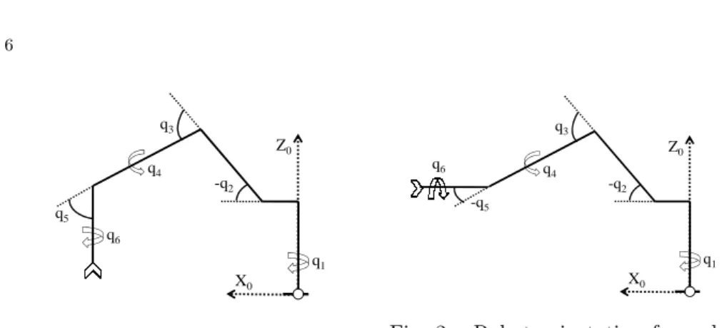
The focus of this article is to improve the performance of standard industrial robot for FSW by taking the advantage of its sufficiently large workspace. For this, KUKA KR 500-MT2 with 6 DOF is considered. Tool (end effector) is located at the 6th axis of the manipulator, which is supposed to be perpendicular to the work piece. We have dealt with welding in both horizontal plane and vertical planes (XY, YZ and ZX), see Fig.1 and Fig.2. The stated model assumes that the links of the manipulator are rigid. Further, only the stiffness in joints is accounted.
Manipulator Kinematics and Dynamics
Calculation by Ulysse [10] shows that, in a FSW process, the axial forces are of order 104N and lateral forces of order 103N. For the initial investigation, a constant ratio between the axial force and the radial force is applied in the simulations in section 4. The generalized force, represented by the vector Ft, is defined in the task frame.
Ft=
[
FtxFtyFtz Mtx MtyMtz
]T
(1) Therefore, it must be transformed w.r.t. the base frame by the transformation re-lation for screws [9]:
Sb→t= [ Rb→t−Rb→tPb→t 0 Rb→t ]T (2) Here, Rb→t defines rotation of task frame with respect to base frame and Pb→t constitutes of position of task frame with respect to base frame. Now, force in base frame Fb can be defined by:
Fb= Sb→tFt (3)
The homogeneous transformation matrix for each joint is defined with Denavit-Hartenberg (DH) parameters, listed in Table. 1. For the ithjoint frame, the direction cosine of the z0
i axis is known from the 3rd column of the transformation matrix (A0
i) (4). The origin of the ith frame is known from p0i vector in the 4th column. So the Jacobian matrix (6) can be built by stacking n (=6) individual columns
Axis α [rad] a [m] θ [rad] d [m] 1 π 0 q1 -1.045 2 π/2 0.5 q2 0 3 0 1.3 π/2 + q3 0 4 -π/2 -0.055 q4 -1.025 5 π/2 0 q5 0 6 -π/2 0 -π/2 + q6 -0.29
consisting of the zi0 vector and zi0× p0E,i vector as discussed in [9]. Here, p0E,i is a vector from the origin of task frame to origin of the ithframe.
A0i = [ x0 i yi0z0i p0i 0 0 0 1 ] (4) p0E,i= p0E− p0i (5) J = [ z0 1 z20 · · · z60 z0 1× p0E,1z 0 2× p0E,2· · · z 0 6× p0E,6 ] (6) The Euler-Lagrange formulation for joint space dynamic model as defined in [9], is given by:
B(q)¨q + C(q, ˙q)q + Fvq + F˙ ssgn( ˙q) + G(q) = τ− JT(q)Fb (7)
where, q is the vector for the joint variables, B constitutes of the inertia matrix of the manipulator, C consists of the centrifugal and Coriolis components, Fv is the viscous friction term, Fs is static friction term, G is the component of torque due to gravity, τ is joint actuation torque and JTF
b represents torque due to force on the end effector.
Some reasonable simplifications have been made during the analysis.(i) Only static analysis has been done (velocity and acceleration in operation is close to zero), (ii) The robot experiences zero viscous friction, (iii) Static friction is also zero. New dynamic equation takes the following shape:
τ = G(q) + JT(q)Fb (8)
Equation (8) relates the torque requirement to guide the end effector under effect of gravity and acting wrench on the end effector which is a function of only joint angles.
Deformation due to Joint Flexibilities
A relation to calculate the errors in position and orientation is derived. For the flex-ible joint model, apart from equation (8), actuation torque can also be represented by:
5
qmis the angle by which the motor rotates, and q is the actual rotation of the link. The difference lies because of finite stiffness, K. This difference is the source of errors we want to quantify in the Cartesian space. Equating the two set of results from equation (8) and (9) and subsequently applying forward kinematics, an estimate of errors in Cartesian space is derived.
qm− q = K−1 ( G(q) + JTFb ) (10) dE = J K−1(G(q) + JTFb ) (11)
dE is 6×1 vector consisting of errors in position (X, Y , Z) and orientation (A, B, C)
in terms of joint parameters. The optimization is based on decreasing this error function which depends on joint angles and varies along the entire workspace of the manipulator. In the next section, we have further tried to simplify this function.
Welding Orientations
We have discussed two cases of welding in horizontal and vertical planes. Depending upon the configuration, there are different constraints on the joint variables. We have also laid emphasis on reducing the number of variables in optimization problem. In fact, not all the joint variables are essentially needed for the calculations because of the reasons mentioned below. Rotation around the 1st joint axis is symmetric. Without loss of generality, q1 can be set to 0 or π/2 depending upon the welding in
yz or xz plane respectively. In each plane of welding: xy, yz or zx, the workpiece
is placed so that joints 4 and 6 can also be set as constant as they affect only the orientation of the tool which we can keep fixed at all times. These constants are chosen as zero again. In fact, this only affects the right term in equation (11) because quite intuitively, gravity term is already independent of q1, q4and q6. When
the welding is to be performed on a horizontal surface, the axis of the end effector remains in (−Z0) vertical direction at all times (Fig. 1). This results in a constraint
relation between the remaining non zero variables, namely q2, q3 and q5.
q5=
π
2 − q2− q3 (12)
In case of welding in vertical plane, axis of end effector always remains horizontal (along x or y in base frame). The constraint relation modifies to:
q5=−q2− q3 (13)
At this stage, effectively, we have been able to reduce the optimization problem to two variables which were six initially.
3. OPTIMIZATION ALGORITHM
Equation (11) can be used to calculate errors in the complete workspace, even for non zero q1, q4 and q6. That’s something irrelevant while we are looking for an
q1 -q2 q3 q4 q5 q6 Z0 X0
Fig. 1. Robot orientation for weld-ing in the xy plane.
q1 -q2 q3 q4 -q5 q6 Z0 X0
Fig. 2. Robot orientation for weld-ing in the xz or yz planes.
we mostly have another set of constraints defining the shape and the length of welding curve, and often, even a condition on starting point of welding and direction of welding. This optimization algorithm specifically handles all of these constraints. So, in the proposition below, we assume we have a prior knowledge about the length and shape of welding curve.
Determining optimal starting position and direction of weld
Welding direction and starting position can both be optimized but in general it is computationally very expensive. To calculate this, one can think of considering many paths emanating from a single starting position. The complexity increases exponentially with the both, the number of directions and the number of starting positions. This is impractical and often, we come across situations where the direc-tion is constrained. For instance, consider the welding of a workpiece in an aeronau-tic application that has been analyzed in section 4 using the proposed approach. Now, we have restricted our discussion in relevance to this application. Given a fixed direction of welding, the objective is to determine optimal starting point. For this, the workspace is discretized in joint coordinates within the geometric bounds governed by the manipulator specifications. Due to the reasons described before, the only variables are q2 and q3. Thus, every combination of (q2, q3) represents a
starting position. This also completes the definition of the required welding path. According to the workspace of the robot KR500-2MT, angles q2 and q3 have
their limits: −130◦ < q2 < 20◦, −94◦ < q3 < 150◦. This range of q2 and q3
has been uniformly divided by considering 7 divisions of q2 and 11 divisions of q3.
This gives a combination of 77 starting points.This choice is defined by considering the calculation time and the precision of the results. In this study, the work piece with a “L” form needs to be welded. With each starting position, errors for 200 intermediate points are then estimated.
Since, welding path is known only in Cartesian space, inverse kinematics is performed on the path to calculate joint coordinates for the intermediate points on the path. Deformation errors can now be easily calculated on path formed by each set of starting positions using equation (11). We chose to minimize the 2-norm of
7
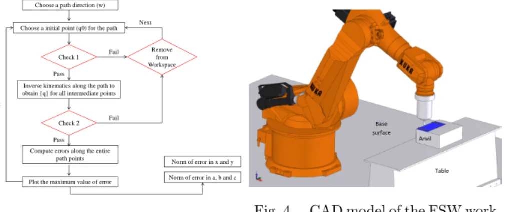
Choose a initial point (q0) for the path
Inverse kinematics along the path to obtain {q} for all intermediate points
Check 1
Compute errors along the entire path points
Plot the maximum value of error Check 2 Next Next Pass Fail Pass Fail Remove from Workspace
Norm of error in x and y
Norm of error in a, b and c Choose a path direction (w)
Fig. 3. Flow chart of the optimiza-tion process
Anvil
Table Base
surface
Fig. 4. CAD model of the FSW work cell.
errors in lateral direction (X, Y if welding is in xy plane) and 2-norm of errors in orientation (A, B, C). Two criteria are defined: C1for the trajectory following error
and C2for the travel angle error. Here, n is the unit normal vector of the considered
welding plane and k is the points number on the paths:
C1= max
k (dE(1 : 3)− dE(1 : 3) • ⃗n) (14)
C2= max
k ∥dE(4 : 6)∥ (15)
Here dE(1 : 3) and dE(4 : 6) refer to the first and last 3 components of dE respec-tively. Leading from all starting positions (j) we determine than the optimal set q∗2 and q∗3 by solving:
(q2∗, q∗3) = arg min
j ∥Ci∥ (i = 1 or 2) (16)
While implementing this method, it has also been ensured that only the results for the feasible data set are evaluated. The set of initial positions are defined as the starting workspace in the optimization process. It is necessary to check if all the starting points remain feasible at all times. So, some intermediate checks have been introduced to reject the unfeasible ones. Firstly, we must maintain the desired orientation for every starting point. We had earlier defined q5 as a function of q2
and q3. But q5 also has its own bounds given by robot characteristics (−118◦ <
q5< 118◦). Therefore, there exist some points which do not satisfy both conditions
simultaneously. Secondly, it must also be ensured that while performing inverse kinematics, the end effector is always inside the robotic workspace. The complete optimization process is summarized in Fig.3.
4. RESULTS
Simulation condition
In real condition of FSW process, there is the “Ground surface” with the “Table” and the “Robot KUKA” fixed on it. The “Sheets” are fixed on the “Anvil”, and the
Fig. 5. Welding direction for different workpiece poses.
Path Minimum of C1 (mm) Minimum of C2 (rad)
x to y 1.300 0.0020 x to z 0.869 0.0028 y to x 1.500 0.0021 y to z 0.930 0.0007 z to x 1.900 0.0027 z to y 1.900 0.0017
welding trajectory is as shown in the picture “Sheet fastenings”. Only the Anvil can be changed on the Table of its placement and orientation. Fig. 4 shows the CAD model of the FSW work cell.
The developed methodology has been applied to a workpiece used in aeronautic applications welded by KUKA KR 500-2MT. Flexibility errors were calculated for 6 particular directions spanning the complete discretized combination of (q2, q3).
There are many possible placements and orientations but it is not necessary to analyze all the possibilities. According to the real condition of FSW, the conditions have been simplified into three orientation of “Anvil” with two directions of welding: for these three different positions of “Anvil”, there are also two differences welding directions, so 6 paths are analyzed: “xtoz”, “ztox”, “ytoz”, “ztoy”, “xtoy” and “ytox” as shown on Fig. 5, e.g. we can weld the workpiece along red or green flash
−→. Because of the effect of gravity, we will get different results for each condition.
Then, the optimal placement and orientation of the work piece can be found out according to the defined criteria.
Comments for results
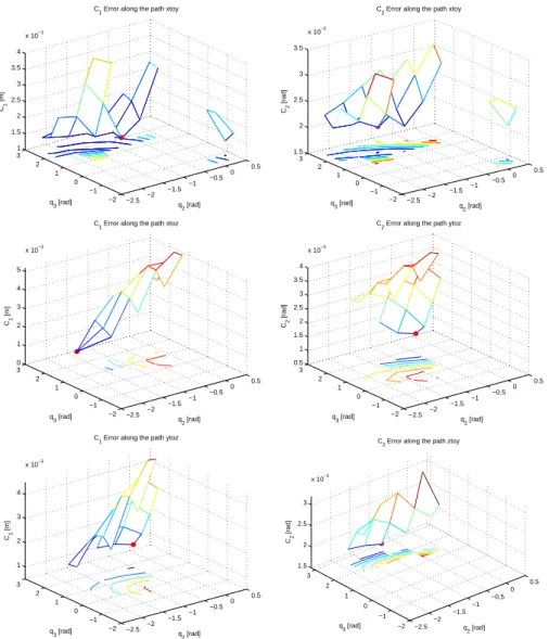
The Fig. 6 presents the value of C1 and C2 during the whole trajectory for each
feasible starting point and different welding directions. Some paths with better results of C1 and C2 are presented. These figures also point out (in red dot) an
optimal starting point for each case. The minimum values of C1 and C2 are also
calculated and given in Table. 4.
Under the given welding condition, a better welding accuracy in posi-tion can be obtained for the path “xtoz” with a starting point equals q0 =
9 [
0−1.833 1.766 0 1.637 0] and in orientation for the path “ytoz” with a starting
point equals q0= [ 0−0.087 2.618 0 −0.960 0][rad]. −2.5 −2 −1.5 −1 −0.5 0 0.5 −2 −1 0 1 2 3 1 1.5 2 2.5 3 3.5 4 x 10⁻³ q2 [rad] C1 Error along the path xtoy
q3 [rad] C1 [m] −2.5 −2 −1.5 −1 −0.5 0 0.5 −2 −1 0 1 2 3 1.5 2 2.5 3 3.5 x 10⁻³ q 2 [rad]
C2 Error along the path xtoy
q3 [rad] C2 [rad] −2.5 −2 −1.5 −1 −0.5 0 0.5 −2 −1 0 1 2 3 0 1 2 3 4 5 x 10⁻³ q2 [rad] C1 Error along the path xtoz
q3 [rad] C1 [m] −2.5 −2 −1.5 −1 −0.5 0 0.5 −2 −1 0 1 2 3 0.5 1 1.5 2 2.5 3 3.5 4 x 10⁻³ q2 [rad] C2 Error along the path ytoz
q3 [rad] C2 [rad] −2.5 −2 −1.5 −1 −0.5 0 0.5 −2 −1 0 1 2 3 1 2 3 4 x 10⁻³ q2 [rad] C1 Error along the path ytoz
q3 [rad] C1 [m] −2.5 −2 −1.5 −1 −0.5 0 0.5 −2 −1 0 1 2 3 1.5 2 2.5 3 x 10⁻³ q2 [rad] C2 Error along the path ztoy
q3 [rad] C2
[rad]
Fig. 6. C1 and C2errors versus starting point coordinates.
5. CONCLUSION
This paper concentrates on an industrial manipulator KUKA KR500 MT-2 for FSW process; the errors in position and orientation have been estimated for different welding directions during task placement. The results show that a difference of 1 mm from the minimum value of C1, and 0.0021 rad from the minimum value
of C2 can be obtained for a different direction of trajectory. Then, for a given
direction, e.g. path x to z, the analysis also shows that the value of C1 varies
from 0.869 mm to 5.8 mm, the value of C2 varies from 0.0028 rad to 0.0047 rad for
different starting points. With the proposed approach, the welding performance can be greatly improved by choosing a better welding direction and starting position. Although, we have analyzed an affine path for the welding, the method can also be applied for complex paths. The results closer to real welding condition can be achieved by using a complete FSW model and robot system.
Acknowledgments
This study is a part of the project ANR-2010-SEGI-003-01-COROUSSO that is sponsored by the French National Agency of Research as a part of the program ANR-ARPEGE.
REFERENCES
1. Smith C.B., “Robotic Friction Stir Welding using a Standard Industrial Robot”,
“Proc. of the 2nd Int. Friction Stir Welding Symposium”, Gothenburg, Sweden,
(27-29 June 2000).
2. Longhurst W.R., Strauss A.M., Cook G.E. and Fleming P.A., “Torque control of friction stir welding for manufacturing and automation”, “International Journal
of Advanced Manufacturing Technology”, Vol. 51, Issue 9-12, (2010), pp. 905-913.
3. Soron M. and Kalaykov I., “A Robot Prototype for Friction Stir Welding”,
“Robotics, Automation and Mechatronics, 2006 IEEE Conference”, Bangkok,
Thailand, 10.1109/RAMECH.2006.252646, (7-9 June 2006), pp 1-5.
4. Bres A., Monsarrat B., Dubourg L., Birglen L., Perron C., Jahazi M. and Baron L., “Simulation of friction stir welding using industrial robots”, “Industrial
Robot: An International Journal”, Vol. 37, Issue 1, (2010), pp. 36-50.
5. Pamanes G.J.A. and Zeghloul S., “Optimal placement of robotic manipulators using multiple kinematic criteria”, “Proceedings of the 1991 IEEE International
Conference an Robotics and Automation”, Sacramento, California, Vol.1, (April
1991), pp. 933-938.
6. Nektarios A. and Aspragathos N.A., “Optimal location of a general position and orientation end-effector’s path relative to manipulator’s base, considering veloc-ity performance”, “Robotics and Computer-Integrated Manufacturing”, Vol. 26, Issue 2, (2010), pp. 162-173.
7. Ur-Rehman R., Caro S., Chablat D. and Wenger P., “Multi-objective path place-ment optimization of parallel kinematics machines based on energy consumption, shaking forces and maximum actuator torques: Application to the Orthoglide”,
“Mechanism and Machine Theory”, Vol. 45, Issue 8, (2010), pp. 1125-1141.
8. Spong M., Hutchinson S. and Vidyasagar M., “Robot Modeling and Control”, John Wiley and Sons, Inc., Berlin Heidelberg, (2005).
9. Craig J.J., “Introduction to Robotics : Mechanics and Control”, 3rd edition, Addison-Wesley, (2004).
10. Ulysse P., “Three-dimensional modeling of the friction stir-welding process”,