HAL Id: tel-00925722
https://tel.archives-ouvertes.fr/tel-00925722
Submitted on 8 Jan 2014
HAL is a multi-disciplinary open access
archive for the deposit and dissemination of sci-entific research documents, whether they are pub-lished or not. The documents may come from teaching and research institutions in France or abroad, or from public or private research centers.
L’archive ouverte pluridisciplinaire HAL, est destinée au dépôt et à la diffusion de documents scientifiques de niveau recherche, publiés ou non, émanant des établissements d’enseignement et de recherche français ou étrangers, des laboratoires publics ou privés.
Michaël Thomazo
To cite this version:
Michaël Thomazo. Conjunctive Query Answering Under Existential Rules - Decidability, Complexity, and Algorithms. Artificial Intelligence [cs.AI]. Université Montpellier II - Sciences et Techniques du Languedoc, 2013. English. �tel-00925722�
Délivré par l’Université Montpellier II
Préparée au sein de l’école doctorale I2S
Et de l’unité de recherche LIRMM
Spécialité: Informatique
Présentée par Michaël Thomazo
Conjunctive Query Answering
Under Existential Rules
Decidability, Complexity, and Algorithms
Soutenue le 24 octobre 2013 devant le jury composé de : Co-directeurs de thèse
M. Jean-François BAGET Chargé de recherche Inria
Mme Marie-Laure MUGNIER Professeur Université de Montpellier
Rapporteurs
M. Georg GOTTLOB Professeur Université d’Oxford
M. Carsten LUTZ Professeur Université de Brême
Mme Marie-Christine ROUSSET Professeur Université de Grenoble
Examinateur
Contents i
List of Figures iii
List of Tables v
Remerciements 1
1 Introduction 3
2 The landscape of OBQA 7
2.1 Representing data and queries . . . 7
2.2 Ontology formalisms . . . 12
2.2.1 Description Logics . . . 12
The Description Logic EL . . . 14
The DL-Lite Family . . . 15
2.2.2 Existential Rules . . . 16
2.2.3 Translation of lightweight DLs into existential rules . . . 17
2.3 Tackling an undecidable problem . . . 18
2.3.1 Materialization-based approaches . . . 19
2.3.2 Materialization avoiding approaches . . . 22
Two kinds of rewritability . . . 22
A generic algorithm for first-order rewritable sets . . . 24
2.3.3 Impact of negative constraints and equality rules . . . 31
2.3.4 Rule with atomic head: a simplifying assumption . . . 31
2.4 Zoology of concrete decidable classes . . . 32
2.5 Roadmap of contributions . . . 43 i
3 Materialization-based approach 47
3.1 Greedy-bounded treewidth sets . . . 50
3.2 An optimal algorithm for gbts . . . 55
3.2.1 Patterned Forward chaining . . . 56
3.2.2 Bag equivalence and abstract bags . . . 59
3.2.3 Abstract patterns and computation of a full blocked tree . . . 62
3.3 Offline and online separation . . . 72
3.3.1 Validation of an APT in a derivation tree . . . 73
3.3.2 Validation of an APT in a blocked tree . . . 78
3.3.3 A bounded validation for APT-mappings . . . 79
Complexity of the algorithm . . . 81
3.3.4 Adaptation to relevant subclasses . . . 82
3.4 Summary, related and further work . . . 83
4 Materialization-avoiding approach 85 4.1 UCQ-rewritings . . . 87
4.1.1 Minimality of a sound and complete UCQ-rewriting . . . 87
4.1.2 Limitation of UCQ-rewritings . . . 88
4.2 USCQ-rewritings: definition and computation . . . 89
4.2.1 Piece-unifiers for semi-conjunctive queries . . . 91
Local and non-local unifiers . . . 92
4.2.2 Gathering tools: COMPACT. . . 93
LU-SATURATION . . . 94
COMPACT . . . 95
An optimization: prime unifiers . . . 98
4.2.3 A close-up on the subsumption test . . . 100
4.3 Experimental evaluation of COMPACT . . . 103
4.3.1 Rewriting step evaluation . . . 104
4.3.2 Querying step evaluation . . . 104
4.3.3 Experimental results . . . 105
4.4 Related and further work . . . 106
5 Conclusion 109
Index 113
2.1 Drawing ofp(a) ∧ t(a, x) ∧ t(x, y) ∧ r(a, z) ∧ s(z, y) . . . 9
2.2 The primal graph of9x9y9z r(x, y) ∧ p(x, z, a) ∧ r(y, z) . . . . 10
2.3 A graph . . . 11
2.4 A tree decomposition of the graph of Figure 2.3 . . . 12
2.5 An infinite chain . . . 20
2.6 The query of the running example . . . 24
2.7 x3being unified with an existential variable (Example 14), dashed atoms must be part of the unification. . . 26
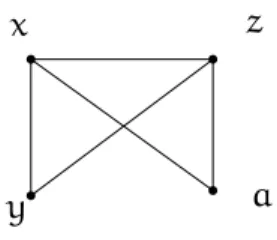
2.8 There is an arrow fromq to q0if and only ifq0is more general thanq. . . 30
2.9 The graph of position dependencies associated with R (Example 21) . . . 36
2.10 The graph of rule dependencies of Example 25 . . . 38
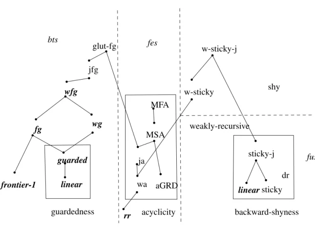
2.11 A summary of decidable classes.The bold italic classes belong to gbts (see Chapter 3). An edge between a lower and an upper class means that the lower class is a syntactic restriction of the upper class. . . 42
3.1 Attempt of building a greedy tree decomposition . . . 51
3.2 The derivation tree associated with Example 28 . . . 52
3.3 Illustration of Example 30 . . . 54
3.4 A graphic representation ofP1b,c. . . 69
3.5 Graphical representation of the rulePb,c1 →Pb,c0 1 . The new element ofPb,c 0 1 is in bold. . . 71
3.6 The full blocked tree associated withFr0 and Rr0. X2andX6are equivalent, as well asX3andX5. . . 74
3.7 A tree generated by the full blocked tree of Figure 3.6. X7 is a copy of X3 underX6. . . 75
3.8 An atom-term partition ofqi: p(x)∧s(x, y)∧r(y, z)∧s(z, t)∧r(t, u)∧r(x, v) 76
4.1 The view associated with the SCQ: (t(x1, x2) ∨ t(x2, x1)) . . . 105
4.2 Querying time for Sygenia generated queries (in seconds) . . . 107
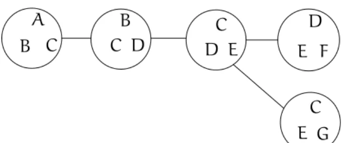
2.1 Translation of (normal) EL-axioms . . . 18
2.2 Translation of DL-Lite axioms . . . 18
2.3 (In-)compatibility results for combinations of decidable classes . . . 40
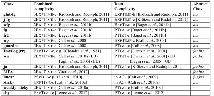
2.4 Combined and Data Complexities . . . 43
4.1 Rewriting time and output for Sygenia queries . . . 106
4.2 Rewriting time and output for handcrafted queries . . . 106
Derniers moments avant la soutenance, me voilà à repenser à ces trois années si riches en rencontres et en expériences. Des années agréables, au cours desquelles j’ai eu la chance d’avoir un encadrement humain et scientifique dont on peut à peine rêver. Merci, Jean-Frano¸is, Marie-Laure d’avoir été des directeurs de thèse parfaits : la porte ouverte lorsqu’il y en a besoin, et quand il le faut, la paix aussi ! Un duo de directeurs complé-mentaires, avec un seul son de cloche quand on en arrive à décider que faire... le rêve ! Du fond du coeur, merci.
Merci également à Georg Gottlob, Carsten Lutz et Marie-Christine Rousset d’avoir accepté de rapporter ma thèse. Vos nombreuses remarques m’ont permis d’améliorer significativement la qualité de ce manuscrit, et j’espère avoir de nouveau l’occasion de discuter avec vous au cours de prochains conférences, réunions de projets, ou peut-être dans d’autres cadres encore ! Merci également à Christophe Paul d’avoir bien voulu être examinateur, après avoir déjà participé à mon comité de suivi de thèse au cours des trois dernières années.
Pas encadrants, et qui pourtant m’ont beaucoup aidé à me cadrer, je dois aussi re-mercier les M&M&M’s (Madalina, Michel et Michel), pour les “pauses” cafés, les dis-cussions à n’en plus finir, et bien entendu, pour animer avec toujours autant d’entrain les réunions d’équipe. Equipe, toujours, comment oublier Bruno, co-bureau atemporel, qui m’a accompagné au sein du labo comme en dehors, en France comme à l’étranger ! Merci également à Annie, dont l’accueil transforme les formalités administratives en un plaisir (très bonne idée, les Pyrénéens, dans ton bureau !). Bien que je ne t’ai pas facilité la tâche au cours de ces trois années entre mes divers déplacements et mon étourderie certaine, tu as continué à me recevoir avec le sourire : merci ! Merci à toute l’équipe GraphIK, des permanents aux stagiaires, en passant bien sûr par les doctorants, les anciens, les actuels et les futurs, pour être ce qu’elle est : une équipe, à mon sens du terme. Au plaisir de vous revoir, bientôt :)
Le LIRMM ne s’arrête cependant pas à l’équipe, et nombre d’autres personnes m’ont accompagné au sein du LIRMM : merci donc à mes compères du Semindoc, Romain (tes affiches font encore la une du labo ;)) et Fabien, pour avoir formé un trinôme au poil. Merci à Petr et Thibaut – binôme parfait pour se changer les idées au besoin ! Merci à Petit Bousquet pour toujours être d’humeur joyeuse, et à Marthe pour les nombreux fruits, gâteaux et thés... Plus généralement, merci aux AlGCo pour entretenir la bonne humeur du couloir ! Arriver au LIRMM veut aussi dire passer par l’accueil, et à ce poste, comment ne pas remercier Laurie et Nicolas ? Sourire, soutien, efficacité... tout est au rendez-vous ! Merci toujours, à l’administration du LIRMM, avec une pensée spéciale pour Caroline, Cécile et Elisabeth – toujours là pour aider quand le besoin s’en fait sentir. Merci, enfin, à la bande d’ECAI’12 – vous vous reconnaîtrez si vous en avez fait partie ! Beaucoup de souvenirs pour une aventure commune inoubliable.
De-zoomons encore un peu plus, car mon environnement de recherche ne s’arrête pas aux mur du LIRMM: remercier toutes les personnes croisées en conférence pour leur accueil chaleureux serait une entreprise vouée à l’échec – je me contenterai donc d’un merci global à eux, et d’un particulier pour les deux chercheurs qui m’ont hébergé durant deux mois chacun: Ken Kaneiwa, à l’université d’Iwate à l’époque (maintenant à The University of Electro-Communications, Tokyo), et Sebastian Rudolph, au KIT à l’époque, et maintenant à la TU Dresden. Ces deux séjours m’ont beaucoup apporté, que ce soit d’un point de vue scientifique ou humain. Merci à vous ! Merci également aux institutions ayant financé ces séjours : la Japan Society for the Promotion of Science (JSPS) pour mon séjour chez Ken Kaneiwa, à travers son excellent programme d’été (ainsi que le CNRS pour la sélection), et la Deutscher Akamedischer Austausch Dienst (DAAD) pour le séjour chez Sebastian Rudolph. Et un deuxième merci à Sebastian, pour ses nombreuses idées, son enthousiasme inébranlable, et la confiance qu’il me témoigne. Que notre collaboration fleurisse !
Une mention spéciale pour Fabienne, du Petit Grain, qui m’a fourni un “bureau” au calme et d’excellents caféS (la majuscule est volontaire) durant la période de rédaction.
Dernière prise de recul : merci à tous ceux qui m’ont accompagné, de près ou de moins près, au cours de ces trois années passées à Montpellier. Rencontrés au labo, à l’escrime, dans un bar, dans un parc, rencontré car c’est l’ami d’une amie d’un ami, que sais-je encore. Merci donc à toutes ces personnes qui m’ont fait me sentir, finalement, chez moi à Montpellier. Je n’ai pas le coeur à oublier quelqu’un dans cette liste (ni même, à vrai dire, de faire une liste) : que ceux qui doivent y être m’invitent donc à prendre un verre, et je pourrais les remercier de vive voix ! Merci, enfin, à la famille (Papa, Maman, Papy, Mamie, Fab, Debi, Babeth, Jean-Louis, Nico et Benji).
Introduction
Exploiting domain knowledge in an automatic way is currently a challenge that draws a lot of attention from both industry and academy. The interest of formal ontologies, which allow to represent this knowledge as logical theories, thus enabling to do reason-ing on it, is now widely recognized. In the context of the Semantic Web, systems and applications based on formal ontologies are in particular made possible by the definition of standards of the W3C, such as OWL (Web Ontology Language) and OWL2.
Existing languages for representing formal ontologies such as OWL/OWL2 are heav-ily based upon Description Logics (DLs). Description Logics are a famheav-ily of languages introduced in the 80’s, that can be seen as decidable fragments of first-order logic. In DLs, domain knowledge is represented by concepts, which are unary predicates in the vocabulary of first-order logic, and roles, which correspond to binary predicates. Sev-eral constructors, depending on the considered DL, are available to build complex con-cepts and roles from atomic ones. Relationships between concon-cepts and roles are stated by means of concept (or role) inclusion axioms. Last, individual elements can be defined, and properties (e.g., of which concept they are an instance) of these individuals may be stated. Historically, most of the studies carried out in DLs have focused on ontologies in themselves, like checking their consistency or classifying a concept with respect to a set of predicates. A guiding principle of the design of DLs has been the search of a good trade-off between the expressivity of the considered DL, and the theoretical complexity of the associated reasoning problems.
The recent years have been marked by a great increase of the volume and the com-plexity of available data. The need for an ontological layer on top of data and for efficient querying mechanisms able to exploit this knowledge has thus become more and more acute. A new reasoning issue, known as ontology-based data access (OBDA), has been brought up: how to query data while taking ontological knowledge into account? Let us give a small example of what we mean by this expression. Assume that a supermarket
opens an online shop. It may sell for instance tofu, lemonade and wasabi-flavored choco-late. The supermarket wants to help customers to find what they are looking for – and enables a semantic search on its catalog. For instance, a vegetarian customer may be es-pecially interested in products that are good protein sources. A direct search on “protein source” and “vegetarian” will not yield any answer, since these terms do not appear in the product descriptions. Using domain knowledge, one can infer that tofu is suitable for a vegetarian, and moreover contains a high share of proteins. This is the kind of inferences that we want to perform when querying data while taking ontologies into account.
Let us stress the three important components that appear in this example. First, we are given an ontology (tofu is a source of proteins,etc), which describes some domain knowl-edge. In this dissertation, we made the choice to represent the ontology by means of
ex-istential rules. Exex-istential rules are positive rules, i.e., they are of the formB → H, where
B and H are conjunctions of positive atoms. No functional symbols appear in existential rules – except for constants – but the head of a rule may contain variables that do not appear in the body, and such variables are existentially quantified. The ability to describe individuals that may not be already present in the knowledge base has been recognized as crucial for modeling ontologies and enable incomplete description of data. Such an ability is not granted within, for instance, Datalog, the language of deductive databases [Abite-boul et al., 1994] but it is in DLs. Existential rules have the same logical form as con-ceptual graph rules [Sowa, 1984; Chein and Mugnier, 2008], as well as tuple-generating dependencies (TGDs) [Abiteboul et al., 1994], which can be seen as Datalog rules ex-tended with existentially quantified variables in the rule head and are one of the building
blocks of the recently introduced Datalog± framework [Calì et al., 2012]. Let us also
mention that existential rules generalize lightweight DLs, which are the most studied DLs in the context of OBDA. Data (the supermarket sells tofu,etc) can be represented using different representational models, such as relational databases, graph databases,etc. We will abstract ourselves from such representations and view data as a formula in first-order logic – more precisely, an existentially closed conjunction of atoms. Last, the queries we consider are conjunctive queries: find a product that is suitable for a vegetarian and is a source of proteins. These queries are considered as basic in the database community: they are both efficiently processed by relational database management systems and often used. Note that all our results can be extended to unions of conjunctive queries (which can be seen in a logical way as a disjunction of conjunctive queries), since to answer a union of conjunctive queries one can simply evaluate each conjunctive query separately. This problem is a particular instance of the ontology-based data access problem, that we will denote by the name ontology-based query answering (OBQA).
In this dissertation, we address the OBQA problem from a theoretical point of view. The presence of existentially quantified variables in the head of rules make this problem undecidable. Classical questions are then the following: what are the most expressive decidable classes of rules that we can design, while keeping decidability of the OBQA problem? Beyond decidability, we are also interested in the worst-case complexity of the problem. Last, we also want to design efficient algorithms for classes of rules that are decidable. The usual approaches to deal with these problems is to use one of the
two following approaches, which we describe here intuitively. A first approach is to “saturate” data, that is, to enrich data in order to add all the information that is entailed by the original knowledge base. A conjunctive query is then evaluated against the saturated data without considering the ontology anymore. This kind of techniques will be called materialization-based in this dissertation. Another popular approach is to reformulate the query into a first-order query using the ontology, and to evaluate this rewritten query directly against the original data. This latter approach is particularly well-suited when the data is so large that materializing all the consequences that can be obtained from the ontology is not reasonable. Moreover, in some cases, the saturated data may be infinite, which prevents from materializing it. However, a similar problem may occur with this materialization-avoiding approach, where no (finite) first-order formula would be a sound and complete rewriting of the original query with respect to the ontology. A more formal description of both approaches, and a landscape of the literature on OBQA are presented in Chapter 2.
The contributions of this dissertation may be split in two parts, according to the two previous kinds of techniques. First, let us give a simple example where the saturated data is not of finite size. We consider a single fact, “Bob is a human”, and a simple ontology, stating that every human has a parent that is a human. We do not discuss the empirical soundness of this rule, but let us focus on the facts that are entailed by our knowledge
base. Being a human, Bob has a parent that is a human. Let us call this parentx1. Since
x1is a human, it also holds thatx1has a parent that is a human, and we can thus state the
existence of an individual x2, that is both a human and a parent of x1. This process can
be repeated as often as we want, creating infinitely many new individuals. The simplicity of the given ontology advocates that this behavior does not only happen in pathological cases. Since we cannot materialize data of infinite size, are we doomed not to be able to answer queries when such ontologies are considered? The answer is already known, and is no: it is in some cases possible to design algorithms to answer conjunctive queries with respect to data and a set of rules even if the saturated data associated to them is not of finite size. One of these cases is when the structure of the saturated data is close to being a tree. However, for some classes of ontologies that ensure tree-likeness of the saturated data, dedicated algorithms are not known yet. We propose a new criterion, which is a structural condition on the saturated data, that ensures decidability of the conjunctive query answering problem. This class of rules covers a wide range of known decidable classes. The intuition behind this condition is that each rule application adds information on individuals that are “close” one to another. We also provide an algorithm that is worst-case optimal for that class of rules, as well as for most of its known subclasses, up to some small adaptations. To achieve this, we present a way to finitely represent the saturated data. This is done by means of patterns. Intuitively, patterns are associated with a set of individuals, and two sets of individuals have equivalent patterns if they are the “root” of similar tree-like structures. This will be developed in Chapter 3.
We also consider materialization-avoiding approaches. A major weakness of most of the rewriting algorithms of the literature is the weak expressivity of the ontologies they support. Indeed, most of them work only for very restricted ontologies. Standing
out is the piece-based rewriting algorithm of [König et al., 2012], that is guaranteed to compute sound and complete rewritings as soon as they exist. However, this algorithm, as well as the majority of others, outputs unions of conjunctive queries. While this is not a restriction in terms of expressivity, we advocate that this is generally not an adequate query language, because of the huge size of the optimal rewritings when large concept and relation hierarchies are present, which is very likely to occur in real-world ontologies. We thus propose to use a more general form of existential positive queries than unions of conjunctive queries, by allowing to use disjunctions in a slightly less restricted way. We also adapt the algorithm of [König et al., 2012] in such a way that it can compute such rewritings, and provide first experiments showing that this approach is more efficient than the classical approach using unions of conjunctive queries. These results are presented in Chapter 4.
The landscape of OBQA
Preamble
In this chapter, we present the ontology-based query answering (OBQA) problem, and a landscape of results about it. We first introduce basic vocabulary about facts, queries and ontologies. We explore links between lightweight description logics and existential rules, which are the two mainly used formalisms to express ontologies when studying OBQA. We last present current approaches for answering queries when taking an ontology into account.
As explained in the previous chapter, the problem we consider in this dissertation is called ontology-based query answering (OBQA). We first need a formalization of its three components: facts, queries and ontologies. After explaining how to represent them, and noticing that the OBQA problem is undecidable in the setting we consider, we present the main known decidability criteria and key concepts used to design classes of rules that fulfill these criteria. We then outline the contributions of this dissertation.
2.1
Representing data and queries
A lot of different technologies allow to store data, among which relational databases, graph databases and triple stores. While relational databases are by far the most used until now, other technologies are also relevant and more appropriate in some application domains – depending on the basic operations that need to be performed on the data. In this dissertation, we abstract from a specific language by considering the formalism of first-order logic. We use its standard semantics, and assume the reader to be familiar with first-order logic, however we recall below some basic notations that will be used throughout this dissertation.
A logical language L = (P, C) is composed of two disjoint sets: a set P of predicates and a set C of constants. Please note that we do not consider functional symbols, except
for constants. We are also given an infinite set of variables V. Each predicate p is
as-sociated with a positive integer, which is called the arity of p. A term on L is either a
constant (i.e., an element of C) or a variable. As a convention, we will denote constants bya, b, c, . . . and variables by x, y, z, . . .. An atom on L is of form p(t1, . . . , tk), where p
is a predicate of P of arityk, and ti is a term on L for anyi. The terms of an atom a are
denoted by terms(a), and its variables are denoted by vars(a). A ground atom contains only constants. The interpretation of a logical language is defined as follows.
Definition 2.1 (Interpretation of a language) An interpretation of a logical language
L= (P, C) is a pair I = (∆, .I) where ∆ is a (possibly infinite) non-empty set called the
interpretation domain and.Iis an interpretation function such that:
1. for each constantc2C, cI2∆;
2. for each predicatep2P of arity k, pI2∆k;
A third condition is sometimes added: two different constants should be interpreted by two different elements of the interpretation domain. This condition is often called the unique name assumption. For the conjunctive query answering problem, it does not change what can be entailed, as long as no equality rules are considered.
We now introduce the notion of fact , which generalizes the usual definition of fact (which is a ground atom), and happens to be convenient in this dissertation.
Definition 2.2 (Fact) Let L be a language. A fact on L is an existentially closed con-junction of atoms on L.
We extend the notions of terms and variables to facts. In the following, we will usu-ally omit the existential quantifiers in the representation of a fact. However, formulas that represent facts should always be considered as existentially closed. Moreover, we will often consider facts as sets of atoms, hence using inclusion and other set theoretic notions directly on facts. Before introducing other concepts, let us provide some examples illus-trating the notion of fact, and clarifying the links between different representations of the same data. This is the purpose of Example 1.
Example 1 Let F be the following first-order formula:
9x9y9z r(x, y) ∧ p(x, z, a) ∧ r(y, z)
where a is a constant. F is a fact, since it is an existentially closed conjunctions of
atoms.
The queries that we consider are conjunctive queries. Such queries are often written a
a p
t x t y
r s
z
Figure 2.1: Drawing ofp(a) ∧ t(a, x) ∧ t(x, y) ∧ r(a, z) ∧ s(z, y)
q = ans(x1, . . . , xk) ← B,
whereB, called the body of q, is a fact, variables x1, . . . , xk occur in B, and ans is
a special predicate, which does not appear in any rule, and whose arguments are used to
build answers. Whenk = 0, the query is a Boolean query, and it is then only described by
its body. In this chapter and in the following, the term query will always denote a Boolean conjunctive query. Restricting ourselves to Boolean queries is not a loss of generality, since conjunctive query answering is classically reducible to Boolean conjunctive query answering.
Facts (and Boolean queries) can be graphically represented, by means of hypergraphs.
Terms of F and atoms of F are respectively in bijection with nodes and hyperarcs of the
corresponding hypergraph. A node is labeled by the name of its corresponding term, and hyperarcs are labeled by the predicate name of the corresponding atom. When facts are only unary or binary, we will represent them as pictured in Figure 2.1. In particular, (hyper)arcs associated with binary atoms are drawn as arcs from the first to the second argument of the atom.
We now introduce the notion of primal (or Gaifman ) graph of a fact, which will be used to lift graph-theoretical notions (such as the treewidth of a graph) to facts. This notion naturally comes from the corresponding notion on hypergraphs: we associate with a fact the primal graph of its hypergraph.
Definition 2.3 (Primal graph) Let F be a fact. The primal graph GF= (VF, EF) of F,
whereVFis the set of vertices ofGFandEFis its set of edges, is defined as follows:
– each term ofF is bijectively associated with an element of VF,
– there is an edge between two vertices of VF if and only if the associated terms
appear in the same atom ofF.
Example 2 (Primal graph) The primal graph of the fact F of Example 1 is given Figure
2.1. It hasx, y, z and a as vertices. The only edge which does not exist is the edge between
y and a, because no atom of F has both y and a as arguments.
A basic problem is the entailment problem, which can be expressed on facts as fol-lows: given two factsF1andF2, is it true thatF1logically entailsF2, i.e., that every model
x
y
z
a
Figure 2.2: The primal graph of9x9y9z r(x, y) ∧ p(x, z, a) ∧ r(y, z)
if and only if there exists a homomorphism fromF2 toF1. A homomorphism from a fact
F to a fact G is a mapping of vars(F) into terms(G) such that atoms are preserved. Definition 2.4 (Substitution, homomorphism, isomorphism) Let X be a set of
vari-ables and T be a set of terms. A substitution σ of X by T is a mapping from X to T .
Given an atom a, σ(a) denotes the atom obtained by substituting each occurrence of
x2 vars(a)\X by σ(x). A homomorphism from a set of atoms S to a set of atoms S0 is
a substitution of vars(S) by terms(S0) such that σ(S)µS0.1 In that case, we say that
S maps to S0
(by σ). An isomorphism from S to S0
is a bijective substitution such that σ(S) = S0.
A well-known fundamental result is the relation between entailment and homomor-phism, which is stated in Theorem 1.
Theorem 1 Let F and F0
be two facts. F0
|= F if and only if there exists a homomorphism fromF to F0
.
In particular, two factsF and F0are logically equivalent if they are homomorphically
equivalent (i.e., there is a homomorphism from one to the other and reciprocally), and this is denoted byF¥F0
. We will sometime refer to the notion of a core of a fact.
Definition 2.5 (Core) A core of a fact F, denoted by core(F), is a minimal (with respect
to inclusion) subset ofF equivalent to F.
It is well-known that all cores of a fact are isomorphic, and we will thus speak about the core of a fact, which is unique up to isomorphism.
Example 3 Let F = r(x, y) ∧ r(x, z) ∧ p(x), where quantifiers have been omitted. The
core ofF is equal (up to isomorphism) to r(x, y) ∧ p(x).
Another graph-inspired notion that we heavily rely upon is the notion of treewidth. This notion, introduced in [Robertson and Seymour, 1986], can be seen as a measurement of how far a graph is from being a tree. Its definition may be introduced by using the notion of tree decomposition.
A B C D E F G Figure 2.3: A graph
Definition 2.6 (Tree decomposition) A tree decomposition of a graph G = (V, E) is a pair ({Xi| i2I}, T = (I, F)) with {Xi| i2I} a collection of subsets of V, called bags, and
T = (I, F) a tree such that:
1. for allv2V, there exists i2I with v2Xi,
2. for all {v, w}2E, there exists i2I such that v, w2Xi,
3. for allv2V, the set Iv= {i2I | v2Xi} forms a connected subtree of T .
The third condition is also known as the running intersection property. The width of a tree decomposition ({Xi| i2I}, T ) is equal to maxi2I| Xi|−1. The treewidth of a graph
G is the minimum width of a tree decomposition of G.
The width is defined by maxi2I| Xi|−1 and not maxi2I| Xi| in order to ensure that
trees have width1.
Example 4 (Tree decomposition) Figures 2.3 and 2.4 present a graph and one of its tree decompositions. One can check that any vertex and any edge belong to a bag. The third
condition is also fulfilled. For example, C belongs to all bags except the (upper)right
most, and these bags form a connected graph. The width of the tree decomposition shown in Figure 2.4 is2.
In order to illustrate the notion of tree decomposition, we recall a simple property that will be useful in Chapter 3. This property is also a simple way of providing (non-optimal) lower bounds on the treewidth of a graph.
Property 1 Let G = (V, E) be a graph. Let X be a clique of G, i.e., a subset of V such that
for any two distinct vertices x and y of X, {x, y} belongs to E. In any tree decomposition
ofG, there exists a bag B such that XµB.
Proof: Let T be a tree decomposition ofG. Let TXbe a minimal subtree of T such that for
A B C B C D D E C D E F G E C
Figure 2.4: A tree decomposition of the graph of Figure 2.3
TXis not restricted to a bag. LetB be an arbitrary leaf of TX. By assumption on TX, there
isx in X such that x is not in B. For any u in B\X, there exists a bag Busuch that bothu
andx are in Bu. By the running intersection property,u belongs also to the parent of B.
Thus,B could be removed from TXwhile keeping a subtree fulfilling the same condition
as TX, which is a contradiction. Thus TXis restricted to a bag, and the claim is proved. ‰
We finally define the treewidth of a fact.
Definition 2.7 (Treewidth of a fact) Let F be a fact. The treewidth of F, denoted by tw(F), is the treewidth of its primal graph.
2.2
Ontology formalisms
In this section, we present two formalisms for representing ontologies. First, Descrip-tion Logics [Baader et al., 2007], the mainstream formalism since the 80’s, are introduced. The focus is put on lightweight DLs, which are the most studied DLs in the framework of OBQA. Second, we present existential rules, which are the basic objects considered in this dissertation. Last, we show how lightweight DLs can be expressed by means of existential rules.
2.2.1
Description Logics
While it is out of the scope of this thesis to propose a comprehensive state of the art of the research done on DLs, it is worth to know that, historically, most studies have focused on the analysis of the ontology itself and not on using it for querying data. In this short presentation of DLs, we present EL and the DL-Lite family, which are called lightweight DLs.
DLs usually encompass two parts: the terminological part, which is called the TBox, and the data, which is called the ABox. The basic objects of a TBox are concepts and roles, which are, in the vocabulary of first-order logic, unary and binary predicates. Prop-erties can be stated about these concepts and roles (such as a role being functional), as
well as relations between roles and concepts. Concepts and roles are inductively defined, starting from atomic concepts and atomic roles. A set of operators allows one to build more elaborated concepts and roles. The expressivity of a DL depends on the set of oper-ators that can be used.
A DL that played a major role in DL research is ALC. Its concepts are built according to the following syntax:
C, D → A |>|?| ¬C | CuD |8R.C |9R.>,
whereA is an atomic concept. The formal semantics of AL-concepts is defined by
means of interpretations I. The logical language of a DL ontology consists in unary and binary predicates (concepts and roles) and constants (in ALC, they appear only in the ABox). An interpretation of such a language is defined as in Definition 2.1, i.e. is
a non-empty set ∆I, called the interpretation domain, and an interpretation function .I.
That interpretation function assigns to each atomic conceptA a subset AIof ∆I, and to
each atomic roleR a subset RIof∆I£∆I. The interpretation function is then extended to
arbitrary concepts in the following way:
>I= ∆I ?I=;
(¬C)I= ∆I\ CI (negation of arbitrary concepts)
(CuD)I= CI\DI (intersection)
(8R.C)I= {a2∆I|8b (a, b)2RI⇒b2CI} (universal restriction)
(9R.>)I= {a2∆I|9b (a, b)2RI} (existential quantification)
More expressive languages could be considered by allowing some other constructors. Those languages are named by adding the corresponding letters to ALC. For instance, one can add:
– union (U):
(CtD)I= CI[DI. – full existential quantification (E):
(9R.C)I= {a2∆I|9b.(a, b)2RI∧ b2CI} – number restrictions (N):
(∏nR)I= {a2∆I| | {b | (a, b)2RI} |∏n}, and
One can also enrich the vocabulary to describe roles. In particular, inverse roles are
used, which are denoted by a “-” as superscript, such as inR−. The influence on semantics
is to exchange the first and the second argument of the role, i.e., the interpretation ofR−
isR−I= {(a, b) | (b, a)2RI}.
Axioms are then defined by concept and role inclusions, functionality axioms, transi-tivity axioms, etc. A concept inclusion is of the following form:
BvC,
and the associated semantics is:
BIµCI
Similarly, a role inclusion is denoted byRvS, and the associated semantics is RIµSI. Questions that have been tackled by the DL community focused on this ontological part: is a concept satisfiable, i.e., is it possible for the interpretation of that concept to be
non-empty? Is a conceptA a subconcept of a concept B, i.e., is it the interpretation of A
a subset of the interpretation ofB? Are two concepts disjoint?
Some reasoning problems may also be defined when taking the ABox into account, which is a set of assertions on individuals, i.e., a set of statements of the following form: A(a) or R(a, b). Queries concerning the ABox are traditionally restricted to very simple queries that consist of a single ground atom. These queries are called instance queries.
Since the problem we consider in this dissertation has been mainly studied for less expressive DLs, we now introduce lightweight description logics. A more detailed and motivated introduction to lightweight description logics can be found in [Baader et al., 2010].
The Description Logic EL
For historical reasons, the first description logics that have been studied all include the possibility to state universal restrictions. However, even with moderately expressive DLs, a basic reasoning problem such as concept inclusion is already PSPACE complete. On the other hand, universal restriction appeared to be far less used than existential restriction in real-world applications.This motivated the study of a novel DL, namely EL [Baader, 2003]. All roles in EL are atomic roles. A concept in EL can be either the top concept (every individual is an instance of the top concept), an atomic concept, the intersection of
two concepts, or a concept9r.C, where r is a role and C an arbitrary concept. A TBox is
a finite set of concept inclusions.
BuCvD,
BvC,
Bv 9R.C,
9R.BvC,
whereB, C and D are atomic concepts. Any EL TBox can be transformed into a TBox
in normal form. This transformation introduces some auxiliary concepts, but entailments on the original vocabulary are preserved [Baader et al., 2005]. This equivalence (up to a given vocabulary) is formalized in Definition 2.29.
EL has nice computational properties: in particular, the subsumption problem
(check-ing if a conceptA is a subconcept of a concept B) is polynomial. On the other hand, it is
still expressive enough to cover important practical cases, as can be witnessed by its use
to model medical ontologies, such as SNOMED-CT.2
The DL-Lite Family
The DL-Lite family has been designed in order to allow efficient conjunctive query answering with large data. The underlying idea is to allow a reformulation of the query: TBox axioms are used to reformulate a conjunctive query into a first-order formula that is directly evaluated against a relational database.
We present three members of the family, namely DL-Litecore, DL-LiteFand DL-LiteR.
A basic role Q is either an atomic role P or its inverse P−. A (general) role R is either
a basic role Q or the negation of a basic role ¬Q. We present the original DL-Lite
[Calvanese et al., 2005]. DL-Lite concepts are defined as follows:
B = A |9R |9R−, C = B | ¬B | C1uC2,
whereA denotes an atomic concept and R denotes an atomic role; B denotes a basic
concept and C denotes a general concept. A DL-Litecore TBox contains assertions of the
following form:
BvC.
A DL-LiteF TBox may also contain functionality axioms, while a DL-LiteA TBox
may contain (basic) role inclusion axioms. 2. http:www.ihtsdo.org/snomed-ct/
2.2.2
Existential Rules
While DLs have been the mainstream formalism to represent and study ontologies from a formal point of view during the last thirty years, other formalisms can be used to represent ontologies. In particular, this is the case of existential rules, which are the main focus of this dissertation. Existential rules – or equivalent objects – have been known under different names: tuple-generating dependencies [Abiteboul et al., 1994], conceptual graph rules [Salvat and Mugnier, 1996], existential rules [Baget et al., 2011a],
Datalog9 rules [Calì et al., 2008],. . . They form the Datalog± framework [Calì et al.,
2009] together with equality rules and negative constraints. The term “Datalog±” makes
clear the syntactic similarity between existential rules and Datalog rules: the “+” means that Datalog rules are extended with existentially quantified variables in the head, while the “-” means that rule bodies are syntactically restricted in order to achieve decidability (or low complexity in some cases).
Definition 2.8 (Existential rule) An existential rule (or simply rule) R = (B, H) on a
lan-guage L is a closed formula of form 8x1. . .8xp(B → 9z1. . .9zq H) where B and H
are two (finite) conjunctions of atoms on L; {x1, . . . , xp}= vars(B); and {z1, . . . , zq}=
vars(H)\ vars(B). Quantifiers are usually omitted, since there is no ambiguity. B and H
are respectively called thebody and the head ofR, also denoted by body(R) and head(R).
Rules are used to infer new knowledge, starting from an initial fact.
Definition 2.9 (Rule application) Let F be a fact and R = (B, H) be a rule. R is said
applicable toF if there is a homomorphism π from B to F. In that case, the application
ofR to F according to π produces a fact α(F, R, π) = F[πsafe(H), where πsafe(x) = x if
π(x) is defined, and is a “fresh”3 variable otherwise. This rule application is said to be
redundant ifα(F, R, π)¥F.
Example 5 presents an example of rule application.
Example 5 (Rule application) Let F = r(a, b)∧p(a)∧s(a, c) and R = p(x) → s(x, y)∧ q(y). R is applicable to F, and its application creates the following fact:
r(a, b) ∧ p(a) ∧ s(a, c) ∧ s(a, y1) ∧ q(y1),
wherey1is a fresh existentially quantified variable.
The notion of frontier of a rule is central in numerous definitions that will be given hereafter. It is the set of variables that are shared by the body and the head of a rule – that is, terms whose image is the set of individuals that are known before the application of the rule and on which (potentially) new knowledge is inferred.
Definition 2.10 (Frontier of a rule) Let R = (B, H) be a rule. The frontier of R, denoted
by fr(R), is the set of variables occurring in both B and H: fr(R) = vars(B)\ vars(H).
Example 6 (Frontier of a rule) The frontier of R = p(x) ∧ s(x, y) → s(y, z) is {y}. We mainly consider “pure” existential rules in this dissertation. However, other kinds
of rules are of interest, and appear in the Datalog±framework: equality rules (also called
equality-generating dependencies, EGDs) and negative constraints. We briefly present them here.
Definition 2.11 (Equality rules) An equality rule R = (H, x = t) is a formula of the form
8x1. . .8xp(H → x = t), where x and t are distinct terms, with x2 vars(H) and t2
vars(H) or is a constant. An application of R on a fact F is a homomorphism π of its
body toF.
We noticed earlier that the unique name assumption does not change the entailments as long as no equality rules are considered. We see here why equality rules may change
this: an equality rule may mapx and t to two different constants, or t may be a constant
andx may be mapped to a different constant. Such an application triggers a failure, and
the knowledge base is logically inconsistent when a failure is triggered.
A special case of equality rules are functional dependencies, which are widely used in data modeling. Such dependencies may express that for a binary atom, if the value of the first argument is set, then the second is also fixed.
Last, negative constraints express that some fact should not be entailed by the
knowl-edge base. In particular, they allow to express concept disjointness. If a and b are two
concepts (unary predicates), one can state that no element can belong to both classes by the following negative constraint:
a(x) ∧ b(x) →?.
Is it worth to study existential rules, since DLs are so well established when dealing with ontologies? A good reason to do so it that this shift of formalism allows one to remove some limitations that are inherent to DLs, but whose incidence on the complexity of the problem that we consider should not be taken for granted. This is in particular the case for predicate arity: DLs consider only predicates that are unary or binary, while there is
a priori no theoretical reason to do so. This is also, and perhaps more importantly, the
case when one wants to represent non-tree shaped structures (as would naturally occur in chemistry for example). This yields sufficient reasons to study the OBQA problem not only from a DL point of view, but also from an existential rule point of view.
2.2.3
Translation of lightweight DLs into existential rules
An interesting feature of existential rules is that they allow to translate lightweight description logics, while preserving their semantics. We present here the translation from
DL-Axiom Translated rule
BuCvD B(x) ∧ C(x) → D(x)
BvC B(x) → C(x)
Bv 9R.C B(x) → R(x, y) ∧ C(y)
9R.BvC r(x, y) ∧ B(y) → C(x)
Table 2.1: Translation of (normal) EL-axioms
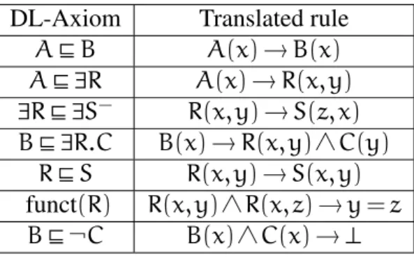
DL-Axiom Translated rule
AvB A(x) → B(x) Av 9R A(x) → R(x, y) 9Rv 9S− R(x, y) → S(z, x) Bv 9R.C B(x) → R(x, y) ∧ C(y) RvS R(x, y) → S(x, y) funct(R) R(x, y) ∧ R(x, z) → y = z Bv¬C B(x) ∧ C(x) →?
Table 2.2: Translation of DL-Lite axioms
these lightweight description logics to existential rules, as can be found in [Calì et al., 2009].
We associate each atomic concept A (resp. basic role R) with a unary (resp. binary)
predicate A (resp. R). Translations of axioms from a normal EL TBox are presented
in Table 2.1, while translations of (some) axioms from a DL-Lite Tbox are presented in Table 2.2. The top concept can also be translated by adding rules for each concept (and each role), stating that every instance of that concept is also an instance of the top concept. Please note that only “pure” existential rules are used in the translation of EL axioms, while equality rules and negative constraints are used to translate functionality and disjointness axioms.
2.3
Tackling an undecidable problem
The core decision problem we consider is the following: given a fact F, a (Boolean)
conjunctive queryq, and a set of rules R, does it hold that:
F, R |= q?
This problem is undecidable [Beeri and Vardi, 1984], even under strong restrictions on sets of rules R [Baget et al., 2011a]. Indeed, it remains undecidable even with a single rule, or with unary and binary predicates. However, several restrictions in the set of rules are known to ensure decidability. Most of there restrictions can be classified in three
categories. The purpose of this section is to present these categories, as well as brute-force algorithms naturally associated with these categories when possible. We first focus on materialization-based approaches, and then explore materialization-avoiding approaches.
2.3.1
Materialization-based approaches
Definition 2.9 explained how to apply a rule to a fact. This section explains how to use this notion of rule application to solve the OBQA problem. We first give an intuitive idea of approaches that can be developed starting from this notion, and formalize these approaches in a second time. The presented procedure is also known as “chase” in the database community.
Rule applications being defined, a natural way to determine if a queryq is entailed by
a KB (F, R) is to infer all possible consequences from F and R, by applying rules of R as
long as possible to infer new information. It is then checked whetherq can be mapped to
the set of atoms thus created. The saturation process is illustrated by Example 7.
Example 7 (Halting forward chaining example) Let us consider the following two rules:
– T : r(xt, yt) ∧ r(yt, zt) → r(xt, zt), which states the transitivity of predicate r;
– R : r(xr, yr) ∧ q(xr) ∧ p(yr) → s(xr, yr, zr).
LetF be the following fact:
F = q(a) ∧ r(a, b) ∧ r(b, c) ∧ r(c, t) ∧ p(t)
Applying all possible rules onF at once results in:
F0= r(a, c) ∧ r(b, t) ∧ F.
Indeed,T can be applied by π1andπ2, where:
– π1(xt) = a, π1(yt) = b, π1(zt) = c,
– π2(xt) = b, π2(yt) = c, π2(zt) = t,
creating respectivelyr(a, c) and r(b, t). On F, no more rules are applicable, but we
can iterate the same process onF0, creatingF00: F00= r(a, t) ∧ F0.
Finally, only one rule application (ofR) can bring new information, which yields:
F§= s(a, t, z) ∧ F00.
In the case of Example 7, a finite number of rule applications is sufficient to infer all consequences of the knowledge base. However, this is not always the case, as can be seen with Example 8, where a single rule is responsible for derivations (Definition 2.12) of unbounded length.
. . . a p t t t t p p p p y0 y1 y2 y3
Figure 2.5: An infinite chain
Example 8 Let R0: q(x) → s(x, y) ∧ q(y). Let F = q(a); R0
is applicable on F,
intro-ducing a new atomp(y), on which R0
is again applicable. This yields an infinite chain of atoms, as illustrated in Figure 2.5.
As we will see later, the non-termination of the saturation process is not a sufficient condition for undecidability of the query answering problem. Specific properties of the so-called canonical model may be used in order to ensure decidability even when this canonical model is not finite. In particular, we will be interested in the treewidth of the canonical model. We now formalize the notions that we have presented so far: the notion of derivation, of saturation, as well as so-called canonical model.
Definition 2.12 (Derivation) Let F be a fact and R be a set of rules. A fact F0
is called
an R-derivation of F if there is a finite sequence (called the derivation sequence) F =
F0, F1, . . . , Fk= F0such that for all i such that 1∑i∑k, there are a rule R = (B, H)2R
and a homomorphismπ from H to Fi−1withFi= α(Fi−1, R, π).
When we saturate a fact with respect to a set of rules, it is convenient to apply rules in a breadth-first manner. Indeed, applying rules in an arbitrary order (in a depth-first manner for example) may lead in a loss of completeness of the proposed approach. Definition 2.13 (k-saturation) Let F be a fact and R be a set or rules. Π(R, F) denotes
the set of homomorphisms from the body of a rule in R toF:
Π(R, F) = {(R, π) | R = (B, H)2R and π is a homomorphism from B to F}.
The direct saturation ofF with R is defined as:
α(F, R) = F[ [
(R=(B,H),π)2Π(R,F)
πsafe(H)
The k-saturation of F with R is denoted by αk(F, R) and is inductively defined by
Saturating a fact until no new rule application is possible allows us to define the
canon-ical modelofF and R, also known in the database community as the universal model. The
particularity of that model is that it maps to any other model ofF and R. In particular, to
check whether a query q is entailed by F and R, it is sufficient to check if the canonical
model ofF and R is a model of q.
Definition 2.14 (Canonical model) Let F be a fact and R be a set of rules. The canonical
model ofF and R, denoted by α∞(F, R) is defined as:
α∞(F, R) =
[
k2N
αk(F, R).
Example 9 By considering Example 7, α0(F, R) = F, α1(F, R) = F0, α2(F, R) = F00,
α3(F, R) = F§= α∞(F, R).
The following theorem is a fundamental tool for solving OBQA.
Theorem 2 ([Baget et al., 2011a]) Let F be a fact, q a query, and R be a set of rules. The following properties are equivalent:
– F, R |= Q;
– there exists a homomorphism fromq to α∞(F, R);
– there isk such that there exists a homomorphism from q to αk(F, R).
We now define two abstract properties of sets of rules, related to the structure of canonical models a set of rules generates. Let R be a set of rules. A first interesting case
is when, for any factF, the canonical model of F and R is equivalent to a finite fact. In
that case, R is called a finite expansion set.
Definition 2.15 (Finite expansion set) A set of rules R is called a finite expansion set (fes) if and only if, for every factF, there exists an integer k = f(F, R) such that αk(F, R)¥
α∞(F, R).
The problem of determining if a set of rules is a finite expansion set is undecidable [Baget et al., 2011a] – it is said that finite expansion sets are not recognizable. Several known subclasses of fes will be presented in the next section. Another abstract class (which is also not recognizable), is the class of bounded treewidth sets. In particular, the canonical model can be of infinite size, as long as it has a tree-like shape.
Definition 2.16 (Bounded treewidth set) A set of rules R is called a bounded-treewidth set (bts) if for any factF, there exists an integer b = f(F, R) such that for any R-derivation F0ofF, the treewidth of core(F0) is less or equal to b.
Notice that the boundb depends on F, which implies that any finite expansion set is
also a bounded treewidth set – it is enough to set b equal to the number of terms of the
where the main argument is a result from Courcelle [Courcelle, 1990], that the OBQA problem is decidable when R is bts.
Let us finish this section by presenting a set of rules that is not bts. Example 10 Let us consider R containing the following two rules:
– R1: p(x) → r(x, y) ∧ p(y),
– R2: r(x, y) ∧ r(y, z) → r(x, z).
LetF be the following fact: {p(a)}. R1is applicable toF, creating in particular a new
atom of predicatep. R1can thus be applied infinitely many times. Let us assume that we
applied itn times. By applying R2 until a fix point is reached, the primal graph of the
obtained fact is a clique of sizen + 1. Since the canonical model of F and R contains a
clique of sizen for any n, its treewidth cannot be bounded.
2.3.2
Materialization avoiding approaches
Another common approach to OBQA relies on a different kind of technique, where no materialization is performed. The main idea is the following: instead of using rules in order to enrich the initial fact, rules are used to rewrite the query. The generated query is then evaluated against the initial fact.
Two kinds of rewritability
One can classify the rewriting techniques existing in the literature in two kinds: rewrit-ing into first-order queries or rewritrewrit-ing into Datalog programs. We successively present both kinds of rewritings.
IfΦ is a class of first-order formula, we define the notion of Φ-rewriting, that will be
used both in this presentation as well as in Chapter 4.
Definition 2.17 (Φ-rewriting soundness/completeness) Let Φ be a class of first-order
formulas, R be a set of rules, andq be a conjunctive query. ϕ2Φ is a sound rewriting
of q with respect to R if for any fact F, it holds that F |= ϕ implies that F,R |= q. ϕ is
acomplete rewriting ofq with respect to R if for any fact F, the converse holds, that is:
F, R |= q implies that F |= ϕ.
The definition of first-order rewritability corresponds to the existence of such a rewrit-ing for any query – without restrictrewrit-ing further the form of the rewritrewrit-ing.
Definition 2.18 (First-order rewritable set of rules) Let R be a set of rules. R is said
to be a first-order rewritable set (F.O.R set) if for any query q, there exists a first-order
sound and complete rewriting ofq with respect to R.
Another, seemingly more restrictive definition, enforces the rewriting to be a disjunc-tion of conjuncdisjunc-tions of atoms, i.e., a union of conjunctive queries (UCQ). We will call such a set of rules a finite unification set. Note that this definition is not the original
definition of finite unification sets, which relies on the finiteness of a given rewriting op-eration. However, we will see in Chapter 4 that the standard definition is equivalent to this one.
Definition 2.19 (Finite unification set) Let R be a set of rules. R is said to be a finite
unification set if for any conjunctive query q, there exists a sound and complete
UCQ-rewriting (that is, a finite set of conjunctive queries) Q, such that for any factF, it holds
thatF, R |= q if and only if there exists q02
Q such that F |= q0
. Such a set Q is called a
sound and complete rewriting ofq with respect to R.
Another strongly related notion has been introduced, called bounded derivation-depth property [Calì et al., 2009]. This notion is presented in the context of a forward-chaining approach, but is highly correlated with finite unification sets.
Definition 2.20 (Bounded derivation-depth property) Let R be a set of rules. R has
the bounded derivation-depth property, if for any query q, there exists an integer γ =
f(q, R) such that for any fact F, if F, R |= q, then αγ(F, R) |= q. In particular, γ depends
only onq and R.
This notion may seem quite close to the definition of a finite expansion set (Definition
2.15). However, the boundγ here does not depend on the initial fact F, whereas it could
depend on it in the case of fes.
As already noted in [Rudolph and Krötzsch, 2013] (for first-order rewritable sets and finite unification sets) these three notions coincide.
Property 2 (Equivalent properties or rule sets) Let R be a set of rules. The following three conditions are equivalent:
1. R is a first-order rewritable set, 2. R is a finite unification set,
3. R enjoys the bounded derivation-depth property.
Not surprisingly, it is undecidable to check if a set of rules is a finite unification set [Baget et al., 2011a].
The other approach uses Datalog programs instead of first-order queries. The litera-ture on Datalog-rewritability has focused on sets of rules that are polynomially rewritable, i.e., that can be rewritten into a program that is of polynomial size in both the query and the set of rules. EL has been shown to be polynomially Datalog-rewritable [Rosati and Almatelli, 2010; Stefanoni et al., 2012], even though EL-ontologies are not first-order rewritable in general. This is also the case for linear and sticky rules [Gottlob and Schwentick, 2012] (see the next section).
s s
t
x1 x2
x3
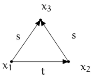
Figure 2.6: The query of the running example
A generic algorithm for first-order rewritable sets
In the remainder of this section, we present a generic algorithm that takes as input any
finite unification set R and any queryq, and outputs a sound and complete rewriting of q
with respect to R. To illustrate the introduced notions, we will rely on Example 11. Example 11 Let Re= {R1, R2, R3, R4, R5}, defined as follows:
– R1: p(x) ∧ h(x) → s(x, y)
– R2: f(x) → s(x, y)
– R3: f1(x) → s1(x, y)
– R4: t(x, y) → t(y, x) – R5: s1(x, y) → s(x, y)
Letqebe the following Boolean query:
qe= t(x1, x2) ∧ s(x1, x3) ∧ s(x2, x3),
whose graphical representation is given Figure 2.6.
Example 11 is designed to be both simple to understand and complex enough to illus-trate the notions we want to introduce.
The algorithm we present now is based on the notion of unification between a query and a rule head. We first recall here the classical definition, as performed by query rewrit-ing approaches (also known as top-down) for (non-existential) Datalog.
Definition 2.21 (Datalog unification) Let q be a conjunctive query, and R be a Datalog
rule. A unifier ofq with R is a pair µ = (a, u), where a is an atom of q and u is a
substi-tution of vars(a)[ vars( head(R)) by terms( head(R))[C s.t. u(a) = u( head(R)).
When a query and a rule unify, it is possible to rewrite the query with respect to that unification, as explained in Definition 2.22.
Definition 2.22 (Datalog rewriting) Let q be a conjunctive query, R be a rule and µ = (a, u) be a unifier of q with R, the rewriting of q according to µ, denoted by β(q, R, µ) is u( body(R)[q¯0), where ¯q0= q \ q0
Please note that these classical notions have been formulated in order to stress simi-larities with the notions we introduce hereafter.
Example 12 (Datalog unification and rewriting) Let us consider qe = t(x1, x2) ∧
s(x1, x3) ∧ s(x2, x3) and R5 = s1(x, y) → s(x, y). A Datalog unifier of qe with R5 is
µd = (s(x1, x3), {u(x1) = x, u(x3) = y}). The rewriting of qe according to µ is the
following query:
t(x, x2) ∧ s1(x, y) ∧ s(x2, y).
Let us stress that this query is equivalent to the following query: t(x1, x2) ∧ s1(x1, x3) ∧ s(x2, x3),
wherex has been renamed by x1andy by x3. In the following, we will allow ourselves
to use such a variable renaming without prior notice.
Applying the same steps without paying attention to the existential variables in rule heads would lead to erroneous rewritings, as shown by Example 13.
Example 13 (False unification) Let us consider qe= t(x1, x2)∧s(x1, x3)∧s(x2, x3) and
R2= f(x) → s(x, y). A Datalog unification of qewithR2isµ error = (s(x1, x3), u(x1) =
x, u(x3) = y). According to Definition 2.22, the rewriting of qewithR2would beqr:
qr= t(x, x2) ∧ f(x) ∧ s(x2, y).
However, qr is not a sound rewriting of qe, which can be checked by performing a
forward chaining mechanism starting from qr considered as a fact. Indeed, R2 can be
applied onqr, creating a new factqr0:
qr0= t(x, x2) ∧ f(x) ∧ s(x2, y) ∧ s(x, y0),
andR4can also be applied, creatingqr00:
qr00= t(x2, x) ∧ t(x, x2) ∧ f(x) ∧ s(x2, y) ∧ s(x, x0).
No further rule is applicable, andqeis not entailed byqr00, which shows thatqris not
a sound rewriting ofqe.
For that reason, the notion of piece unifier has been introduced, originally in the con-text of conceptual graph rules [Salvat and Mugnier, 1996], then recast in the framework of existential rules [Baget et al., 2011a]. Instead of unifying only one atom at once, one may have to unify a whole “piece”, that is, a set of atoms that should have been created by the same rule application. The following definitions and the algorithm are mainly taken from [König et al., 2012].
s s
t
x1 x2
x3
Figure 2.7:x3being unified with an existential variable (Example 14), dashed atoms must
be part of the unification.
Definition 2.23 (Piece unifier) Let q be a conjunctive query and R be a rule. A piece unifier ofq with R is a pair µ = (q0, u) with q0µq, q06=;
, andu is a substitution of
fr(R)[ vars(q0) by terms( head(R))[C such that:
1. for allx2 fr(R), u(x)2 fr(R)[C (for technical convenience, we allow u(x) = x);
2. for allx2 sepq(q0
), u(x)2 fr(R)[C;
3. u(q0)µu( head(R));
where sepq(q0) denotes the set of variables that belongs both to q0and toq \ q0. Let us consider the unification attempted in Example 13 from this point of view. Example 14 (Piece unifier) Let us consider qe = t(x1, x2) ∧ s(x1, x2) ∧ s(x2, x3) and
R2= f(x) → s(x, y). µ0
error = (q0= {s(x1, x3)}, u(x1) = x, u(x3) = y), defined in
Exam-ple 13, is not a piece unifier. Indeed,x3 belongs to sepqe(q
0
), and appears in s(x2, x3),
which does not belong toq0, violating the second condition of piece unifiers.
A correct choice of piece is illustrated Figure 2.7. Letµ = (({s(x1, x3), s(x2, x3)}, u(x1) =
x, u(x3) = y, u(x2) = x). µ is a piece unifier of qe with R2, which can be checked by
verifying that conditions1 to 3 are fulfilled.
Given that definition of unifiers, the definition of rewritings remains syntactically the same as in the Datalog case.
Definition 2.24 (Rewriting) Given a conjunctive query q, a rule R and a piece
uni-fier µ = (q0, u) of q with R, the rewriting of q according to µ, denoted by β(q, R, µ)
isu( body(R)[q¯0), where ¯q0= q \ q0 .
Example 15 (Rewriting) Let µ be the unifier of qe withR2 defined in Example 14. The
rewriting ofqewith respect toµ is:
β(qe, R2, µ) = t(x, x) ∧ f(x).
The notion of R-rewriting allows us to denote queries that are obtained thanks to successive rewriting operations.
Definition 2.25 (R-rewriting of q) Let q be a conjunctive query and R be a set of
rules. An R-rewriting of q is a conjunctive query qk obtained by a finite sequence
q0 = q, q1, . . . , qk such that for all i such that 0∑i <k, there is Ri2R and a piece
unifierµiofqiwithRisuch thatqi+1= β(qi, R, µi).
We now present the fundamental theorem justifying the notion of R-rewriting. This theorem was originally written in the framework of conceptual graph rules. However, the logical translation of conceptual graph rules is exactly existential rules.
Theorem 3 (Soundness and completeness) ([Salvat and Mugnier, 1996]) Let F be a
fact, R be a set of existential rules, and q be a Boolean CQ. Then F, R |= q iff there is
an R-rewritingq0
ofq that F |= q0 .
Before presenting an algorithm for computing a sound and complete rewriting of a
query q with respect to a fus R, let us introduce the notion of original and generated
variables in a rewriting.
Definition 2.26 (Original and generated variables) Let q be a query, R be a set
of rules, and q0
be an R-rewriting of q, obtained by a rewriting sequence q =
q0, q1, . . . , qn= q0. Original variables ofq0(with respect toq) are inductively defined as
follows:
– all variables ofq are original;
– ifqi has original variablesX, and qi+1 is the rewriting of qi with respect to µ =
(q0
i, u), the original variables of qi+1are the images of the elements ofX by u.
A variable that is not original isgenerated.
We recall thatq2|= q1if and only if there is a homomorphism fromq1toq2, which
we denote by q1∏q2. Letq be a CQ, and Q be a sound and complete UCQ-rewriting
of q. If there exist q1 and q2 in Q such thatq1∏q2, then Q \ {q2} is also a sound and
complete rewriting of q. This observation motivates the definition of cover of a set of
first-order queries.
Definition 2.27 (Cover) Let Q be a set of conjunctive queries. A cover of Q is a set
QcµQ such that:
1. for anyq2Q, there is q02Qcsuch thatq0∏ q,
2. elements of Qcare pairwise incomparable with respect to∏.
Example 16 Let Q = {q1= r(x, y)∧t(y, z), q2= r(x, y)∧t(y, y), q3= r(x, y)∧t(y, z)∧
t(u, z)}. A cover of Q is {q1}. Indeed, q1∏q2andq1∏q3, because fori2{2, 3}, π1→i is
a homomorphism fromq1toqi where:
– π1→2(x) = x, π1→2(y) = π1→2(z) = y, and
Algorithm 1 is a generic breadth-first rewriting algorithm, that generates for any query q and any finite unification set R a sound and complete UCQ-rewriting of q with respect
to R. Generated queries are queries that belong to Qtat some point; explored queries are
queries that belong to QE at some point, and thus, for which all one-step rewritings are
generated. At each step, a cover of explored and generated queries is computed. This means that only most general queries are kept, both in the set of explored queries and in
the set of queries remaining to be explored. If two queriesq1andq2are homomorphically
equivalent, and onlyq1 has already been explored, then q1 is kept andq2 is discarded.
This is done in order not to explore two queries that are comparable by the most general relation – which ensures the termination of Algorithm 1.
Algorithm 1: ABREADTH-FIRST REWRITING ALGORITHM
Data: A fus R, a conjunctive query q
Result: A cover of the set of R-rewritings of q QF:= {q}; // resulting set
QE:= {q}; // queries to be explored
while QE6=;do
Qt:=;; // queries generated at this rewriting step for qi2QE do
for R2R do
for µ piece-unifier of qiwithR do
Qt:= Qt[β(qi, R, µ);
Qc:= cover(Q
F[Qt);
QE:= Qc\QF; // select unexplored queries from the cover QF:= Qc;
return QF
Let us execute step by step Algorithm 1 on the running example.
Example 17 Initially, QF= QE= {qe= t(x1, x2) ∧ s(x1, x3) ∧ s(x2, x3)}. Since QE is not
empty, we initialize Qt to the empty set, and consider every element of QE. The only
element of QE isqe, so we add to Qtall possible rewritings ofqe. These are:
– q1= t(x, x)∧p(x)∧h(x), (by unifying) with respect to µ1= ({s(x1, x3), s(x2, x3)}, u1(x1) =
u1(x2) = x, u1(x3) = y), unifier of qewithR1;
– q2= t(x, x) ∧ f(x), with respect to µ2= ({s(x1, x3), s(x2, x3)}, u2(x1) = u2(x2) =
x, u2(x3) = y) , unifier of qewithR2;
– q3 = t(x2, x1) ∧ s(x1, x3) ∧ s(x2, x3) with respect to µ3 = ({t(x1, x2), u3(x1) =
y, u3(x2) = x), unifier of qewithR4;
– q4= t(x1, x2) ∧ s1(x1, x3) ∧ s(x2, x3) with respect to µ4 = ({s(x1, x3)}, u4(x1) =
x, u4(x3) = y), unifier of qewithR5;
– q5= t(x1, x2) ∧ s(x1, x3) ∧ s1(x2, x3) with respect to µ5 = ({s(x2, x3)}, u5(x2) =