ÉCOLE DE TECHNOLOGIE SUPÉRIEURE UNIVERSITÉ DU QUÉBEC
THESIS PRESENTED TO
ÉCOLE DE TECHNOLOGIE SUPÉRIEURE
IN PARTIAL FULFILLMENT OF THE REQUIREMENTS FOR A MASTER’S DEGREE IN ENVIRONMENTAL ENGINEERING
M. Eng.
BY
Gary Paul MOODY
REDUCING PARTICULATE MATTER EMISSIONS FROM RESIDENTIAL WOOD BURNING STOVES BY ELECTROSTATIC PRECIPITATION: A CFD MODELING
STUDY
MONTREAL, DECEMBER 1, 2010
THIS THESIS HAS BEEN EVALUATED BY THE FOLLOWING BOARD OF EXAMINERS
Dr. Robert Hausler, project supervisor
Département de génie de la construction à l’École de technologie supérieure
Dr. Patrice Seers, board president
Département de génie mécanique à l’École de technologie supérieure
Dr. Mathias Glaus, board member
Département de génie de la construction à l’École de technologie supérieure
THIS THESIS HAS BEEN PRESENTED AND DEFENDED BEFORE A BOARD OF EXAMINERS AND PUBLIC
NOVEMBER 2, 2010
RÉDUCTION DES ÉMISSIONS DE PARTICULES FINES PROVENANT DES POÊLES À BOIS PAR MOYEN DE PRÉCIPITATION ÉLÉCTROSTATIQUE:
UNE MODÉLISATION NUMÉRIQUE Gary Paul MOODY
RÉSUMÉ
Les émissions de matière particulaire fine (MP2.5) provenant des poêles à bois résidentiels
sont une source majeure de pollution atmosphérique en Amérique du nord et en Europe du nord en hiver. Cette pollution a été liée à de nombreux problèmes de santé respiratoires. Nous pouvons réduire ces émissions par l’utilisation d’un précipitateur électrostatique (PES) à la sortie du tuyau d’échappement des gaz de combustion. Cette étude avait comme hypothèse qu’un tel dispositif pouvait opérer de façon efficace et ainsi contribuer à une réduction substantielle des émissions de particules fines provenant du secteur de chauffage au bois résidentiel. Un modèle numérique en 2-D d’un PES a été crée et simulé avec un logiciel commercial de mécanique des fluides numériques. Le modèle et le procédé comportaient plusieurs améliorations par rapport aux modèles trouvés dans la littérature, dont : l’utilisation d’une distribution de particules polydispersées, l’utilisation d’un écoulement semi-établi à l’admission des gaz et l’utilisation d’un modèle de chargement des particules qui tient compte des chargements par diffusion et par champs. La technique a été validée par des données expérimentales, et les valeurs de rendement correspondaient avec moins de 5% d’écart aux valeurs expérimentales. Un modèle de référence basé sur les dimensions d’un tuyau d’échappement standard de 0,15 m de diamètre a été simulé et le rendement global était de 75%. L’utilisation répandue de ce dispositif pourrait mener à une réduction de 64% des émissions de MP2.5 provenant du secteur de chauffage au bois résidentiel au Québec. Il y
a plusieurs défis opérationnels et de sécurité qui doivent être surmontés avant de pouvoir commercialiser un tel dispositif.
Mots-clés : particules fines, précipitation électrostatique, modélisation, mécanique des fluides numérique.
REDUCING PARTICULATE MATTER EMISSIONS FROM WOOD BURNING STOVES BY ELECTROSTATIC PRECIPITATION: A CFD MODELING STUDY
Gary Paul MOODY ABSTRACT
Emissions of PM2.5 from residential fuel wood heating appliances are a major source of
winter air pollution in many parts of North America and northern Europe. This pollution has been linked to respiratory health problems. One possible method of reducing these emissions is via an electrostatic precipitator (ESP) installed at the top of the flue pipe of the appliance. This study investigated the hypothesis that such a device can operate efficiently and contribute to a significant reduction in PM2.5 emissions from fuel wood combustion. A 2-D
axisymmetric numerical model of an ESP was created and simulated using commercial computational fluid dynamics software. The model and simulation procedure included several enhancements over similar studies found in the literature such as: the use of a poly-disperse particle distribution, the use of a partially developed gas flow velocity profile and the use of a sum-of-charges particle charging model that includes diffusion and field charging mechanisms. The simulation technique was validated using experimental data and provided collection efficiency values within 5% of the experimental values. A reference model based on the dimensions of a standard flue pipe (diameter of 0,15 m) was simulated and found to have an overall collection efficiency of 75%. Based on these results, the emissions of PM2.5 from residential fuel wood combustion in Quebec province could be
reduced by 64% in one scenario. Several safety and operational issues need to be resolved before such a device can be launched commercially.
Keywords: particulate matter, simulation, electrostatic precipitation, computational fluid dynamics.
TABLE OF CONTENTS
Page
INTRODUCTION ...1
CHAPTER 1 REVIEW OF THE LITERATURE ...4
1.1 Wood fuel combustion and its effects ...4
1.1.1 Ambient PM levels ...5
1.1.2 Fuel wood use and air pollution ...6
1.1.3 Health effects of wood combustion ...6
1.2 Particulate emissions from wood combustion ...8
1.2.1 Formation & characterization of particulate matter ...8
1.2.2 Experimental data from biomass combustion ...12
1.2.3 Particulate emissions control methods ...14
1.2.4 Electrostatic precipitators ...18
1.3 Simulation techniques ...21
1.3.1 Computational Fluid Dynamics overview ...22
1.3.2 CFD simulation of an ESP ...22
CHAPTER 2 METHODOLOGY ...24
2.1 The ESP model ...24
2.1.1 Gas flow field ...25
2.1.2 Electrostatics in a 2-D axisymmetric geometry ...26
2.1.3 Particle charging ...32
2.1.4 Particle trajectories ...35
2.1.5 Computational grid generation ...37
2.1.6 Model creation using UDF macros ...39
2.2 Simulation procedure ...41
2.2.1 Initial values and boundary conditions ...41
2.2.2 DPM injection setup ...42
2.2.3 Solution process ...43
2.2.4 ESP collection efficiency evaluation ...46
2.2.5 Model validation ...47
2.2.6 Assumptions & limitations ...48
2.3 Electrostatic precipitator simulation models ...49
2.3.1 Reference model ...49
2.3.2 Prototype model ...50
CHAPTER 3 RESULTS ...51
3.1 Validation model results ...51
3.1.1 Model geometry and parameters ...51
3.1.2 Voltage-current curves ...52
3.1.4 ESP collection efficiency curve ...58
3.1.5 Variation of ηov with applied voltage and gas flow velocity ...59
3.2 Reference model results ...61
3.2.1 Model geometry and parameters ...62
3.2.2 Voltage-current curves ...63
3.2.3 Simulation results...64
3.2.4 ESP collection efficiency curve ...69
3.2.5 Variation of ηov with applied voltage and gas flow velocity ...70
3.3 Prototype model results ...71
3.3.1 Model geometry and parameters ...71
3.3.2 Voltage-current curves ...73
3.3.3 Simulation results...74
3.3.4 ESP collection efficiency curves ...79
3.3.5 Variation of ηov with applied voltage and gas flow velocity ...80
3.3.6 Total performance characteristics of the prototype model ...81
3.4 Model performance comparison ...82
CHAPTER 4 DISCUSSION ...84 4.1 Modeling techniques ...84 4.2 The simulations ...87 4.2.1 Validation model ...87 4.2.2 Reference model ...88 4.2.3 Prototype model ...90 4.2.4 Model comparison ...90
4.3 PM emissions reduction estimate ...91
4.4 Practical & design considerations ...91
CONCLUSION ...93
APPENDIX I UDF MACRO SOURCE CODE ...95
APPENDIX II EXAMPLE EXCEL MACRO FOR DATA IMPORT ...103
APPENDIX III GAS FLOW VELOCITY PROFILE IN A FLUE PIPE ...106
APPENDIX IV PARTICLE SIZE DISTRIBUTION GRAPHS ...108
APPENDIX V CONTOUR PLOTS FOR THE PROTOTYPE MODEL, UINLET = 0,77 m/s ...110
LIST OF TABLES
Page Table 1.1 Compositional analysis of PM from residential wood combustion for
three wood species ...10
Table 1.2 Summary table of emissions control devices and characteristics ...16
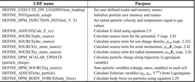
Table 2.1 List of FLUENT UDF macros written to build the ESP model ...40
Table 2.2 ESP model boundary conditions used during the simulation ...42
Table 2.3 List of variables solved during the iteration process ...44
Table 3.1 Validation ESP model parameters and constants ...51
Table 3.2 Reference ESP model parameters and constants ...62
LIST OF FIGURES
Page
Figure 1.1 Constituents of PM from oak combustion, as percentage of total PM mass. ...11
Figure 2.1 Schematic diagram of the main components and interactions in an ESP. ...24
Figure 2.2 Schematic of the wire-cylinder geometry. ...27
Figure 2.3 Plan view of a cylindrical ESP. ...29
Figure 2.4 Schematic view of the 2-D axisymmetric computational domain. ...37
Figure 2.5 The computational grid of the reference model near the inlet. ...38
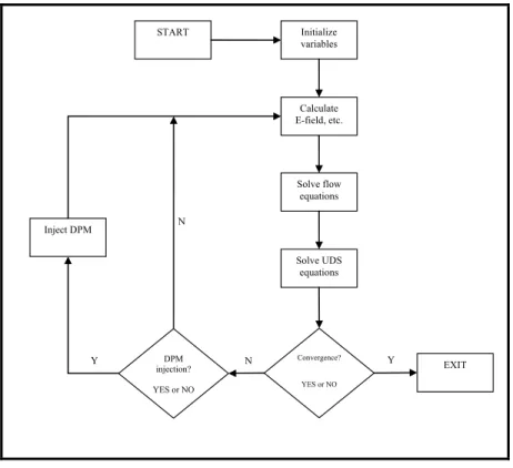
Figure 2.6 Flow chart of the FLUENT solution process for the ESP simulation. ...45
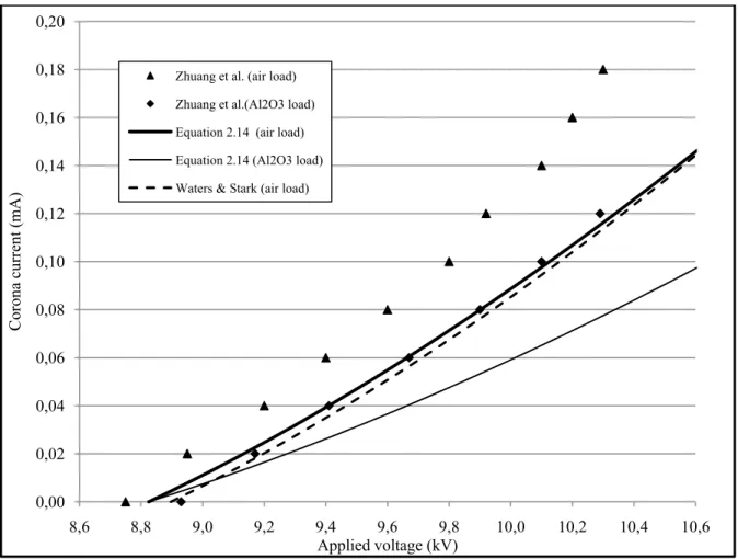
Figure 3.1 Corona current as a function of applied voltage, as measured by Zhuang et al. and from theoretical relations by Waters and Stark (1975) and Oglesby and Nichols (1970) for the validation model ESP. ...53
Figure 3.2 Gas flow variables for the validation model simulation: (a) Static pressure field (Pa), (b) Axial gas velocity (m/s), (c) Radial gas velocity (m/s), (d) Turbulence intensity (%). ...55
Figure 3.3 Electrostatic variables for the validation model simulation: (a) Electric potential (V), (b) Electric field strength (V/m), (c) Ion charge density (C/m3). ...56
Figure 3.4 Particle Eulerian variables for the validation model simulation: (a) particle number concentration (m-3), (b) particle mass concentration (kg/m3), (c) particle charge density (C/m3). ...57
Figure 3.5 ESP collection efficiency curves as measured by Zhuang et al. and as obtained from the validation model simulation. ...59
Figure 3.6 Overall ESP collection efficiency of the validation model as a function of applied voltage for the given model parameters. ...60
Figure 3.7 Overall ESP collection efficiency of the validation model as a function of the inlet gas flow velocity for the given model parameters. ...61
Figure 3.8 Corona current as a function of applied voltage for the reference model, from theoretical relations by Waters and Stark (1975) and Oglesby and Nichols (1970). ...64
IX
Figure 3.9 Gas flow variables for the reference model simulation: (a) Static pressure field (Pa), (b) Axial gas velocity (m/s), (c) Radial gas velocity (m/s),
(d) Turbulence intensity (%). ...66 Figure 3.10 Electrostatic variables for the reference model simulation: (a) Electric
potential (V), (b) Electric field strength (V/m),
(c) Ion charge density (C/m3). ...67 Figure 3.11 Particle Eulerian variables for the reference model simulation: (a) particle
number concentration (m-3), (b) particle mass concentration (kg/m3),
(c) particle charge density (C/m3). ...68 Figure 3.12 The ESP collection efficiency curve as a function of particle diameter
obtained from the reference model simulation. ...69 Figure 3.13 Overall ESP collection efficiency curves for the reference model as a
function of applied voltage for three gas flow velocities at the inlet. ...70 Figure 3.14 Cross-sectional view of the prototype ESP geometry, showing multiple
ESP tubes inside the main flue pipe, and the gas velocity profile used in
the simulation. ...72 Figure 3.15 Corona current as a function of applied voltage for the prototype model,
from theoretical relations by Waters and Stark (1975) and Oglesby and
Nichols (1970). ...74 Figure 3.16 Gas flow variables for the prototype model simulation with an inlet gas
velocity of 1,0 m/s : (a) Static pressure field (Pa), (b) Axial gas velocity
(m/s), (c) Radial gas velocity (m/s), (d) Turbulence intensity (%). ...76 Figure 3.17 Electrostatic variables for the prototype model simulation with an inlet gas
flow velocity of 1,0 m/s : (a) Electric potential (V), (b) Electric field
strength (V/m), (c) Ion charge density (C/m3). ...77 Figure 3.18 Particle Eulerian variables for the prototype model simulation with an inlet
gas flow velocity of 1,0 m/s : (a) particle number concentration (m-3),
(b) particle mass concentration (kg/m3), (c) particle charge density (C/m3). ....78 Figure 3.19 The ESP collection efficiency curve as obtained from the prototype model
simulation for two inlet gas flow velocities. ...79 Figure 3.20 Overall ESP collection efficiency of the prototype model as a function of
applied voltage for the two simulations with inlet gas velocities of 0,77
and 1,0 m/s. ...80 Figure 3.21 Overall ESP collection efficiency of the prototype model as a function of
Figure 3.22 Total ESP collection efficiency of the prototype device as a function of the applied voltage, based on a velocity profile with a maximum value of
1,0 m/s. ...82 Figure 3.23 Overall ESP collection efficiency as a function of the estimated power
consumption for the reference and prototype models, based on a velocity profile with an average value of 0,84 m/s. ...83
LIST OF ABREVIATIONS, INITIALS AND ACRONYMS CFD Computational fluid dynamics
CMD Count median diameter
CNC Condensation nucleus counter
CWS Canada-wide standards
DC Direct-current
DMA Differential mobility analyser DPM Discrete phase model
EPA U.S. Environmental Protection Agency ES Electrostatic
GC-MS Gas-chromatography and mass spectrometry GUI Graphical user interface
IARC International Agency for Research on Cancer
ICRP International Commission on Radiological Protection MFP Mean free path
MMD Mass median diameter
NAAQS National Ambient Air Quality Standard NFR Number flow rate
N-S Navier-Stokes equations
PDE Partial differential equation
PM Particulate matter
PM2.5 Fraction of PM captured with 50% efficiency at diameter 2,5 µm
and greater efficiency at smaller diameters
UCM Unresolved complex mixture
UDF User defined function UDS User defined scalar
LIST OF SYMBOLS AND UNITS OF MEASURE Scalar quantities
Axs cross-sectional area of the ESP (m2)
a particle dielectric factor
Be(p) dimensionless diffusion charging rate
beq equivalent mobility (m2/V/s)
bion ion electrical mobility (m2/V/s)
Cc Cunningham slip correction factor
De effective ion diffusivity (m2/s)
ion diffusion coefficient, (kg/m/s)
dp particle diameter (m)
Ec critical value of the electric field at the wire surface (V/m)
e electronic charge (C)
F(p,w) dimensionless field charging rate
I total current (A)
i current per unit length (A/m)
k Boltzmann’s constant (J/K)
mp particle mass (kg)
particle mass flow rate (kg/s)
N number of particle injection streams entering cell
Np total particle number density (m-3)
total number of particles injected into the domain
n particle injection index
nc integer number of elementary charges
number of particles captured for each tracking sample
fractional number density for the given particle diameter (m-3)
particle number flow rate for particle diameter dp (s-1)
nt number of tries for stochastic tracking
P static gas pressure (Pa)
p dimensionless charge
p0 standard pressure (101 325 Pa)
qp total charge on a particle (C)
R radius of the outer cylinder (m)
r radial distance from the wire surface (m)
rp particle radius (m)
rw wire radius (m)
S ESP collection surface area (m2)
Sm mass source term (kg/m3/s)
Sφ source term for scalar variable φ
ion charge density source term ( C/m3/s)
T0 standard temperature (293 K)
Tp particle temperature (K)
XIII
mean axial gas flow speed (m/s)
V applied voltage at the wire (V)
Vc cell volume (m3)
volume flow rate (m3/s)
w dimensionless electric field magnitude Greek symbols
∆ particle residence time in a cell (tout – tin)
δ non-standard temperature and pressure correction factor
εo permittivity of free space (F/m)
εr dielectric constant
overall weighted-average collection efficiency (%)
η collection efficiency (%)
fractional collection efficiency for particle size dp
λ molecular mean free path of the carrier gas (m)
µ fluid dynamic viscosity (kg/m/s)
ρ mass density of the flue gas (kg/m3)
ρion ion charge density (C/m3)
ρp particle mass concentration (kg/m3)
ρpc particle charge density (C/m3)
ρtot total space charge density (C/m3)
σg geometric standard deviation
τ dimensionless time
φ FLUENT scalar variable Vector quantities (bold)
B vector sum of body forces per unit volume (N/m3), E electrostatic field (N/C or V/m)
FD aerodynamic drag force (N/m3)
FES electrostatic force acting on the particle (N)
Fg gravitational force (N)
g gravitational acceleration (m/s2) j total current density (A/m2) jion ion current density (A/m2)
jp particle current density (A/m2)
U gas flow velocity vector (m/s)
v Lagrangian particle velocity vector (m/s) Vcell Eulerian particulate velocity vector (m/s)
INTRODUCTION
The current scientific consensus regarding global climate change is that urgent action is needed to reduce energy use from fossil fuels and develop alternative sources. Since wood can be classified as a renewable, carbon neutral resource (excluding harvesting and transportation) it will most likely gain in popularity over the coming years in North America and elsewhere. The reasons for this are the relative abundance of wood resources and the existing infrastructure in the form of residential fireplaces and wood stoves. It is also seen as a less costly option in the short term than installing a cleaner system such as a geothermal heat pump.
According to data published by Environment Canada (2009), wood burning for residential heating in Quebec during 2007 produced well over half of the total man-made atmospheric particulate matter (PM) emissions in the size range below 2,5 µm, commonly referred to as PM2.5. This is the concentration of PM captured with 50% efficiency at diameter 2,5 µm and
greater efficiency at smaller diameters. These PM2.5 emissions are one of the main causes of
urban smog events in large urban centres such as the greater Montreal area. Smog events are an indicator of poor air quality, with subsequent effects on the health of the population. Currently, smog alerts are issued on a regular basis during the winter in the Montreal metropolitan area. Any increase in the use of wood for residential heating will most likely lead to an increase the number of smog alerts. During a smog alert, the population is advised not to burn wood, however, with the exception of the borough of Hampstead, there are no strictly enforced municipal by-laws prohibiting wood burning during smog events in the Montreal area. In April 2009, the City of Montreal (2009) took the step of adopting a municipal by-law banning the installation of new solid fuel stoves in residential properties. This by-law may prevent the situation from worsening in the future, but it does nothing to reduce the problem caused by the estimated 50,000 wood burning stoves currently installed on the island of Montreal alone.
2
A particularly difficult situation is when a smog alert is issued during a very cold spell lasting several days, as occurred in Montreal during the winter of 2008/2009, when the smog episode lasted 4 days. When the demand on the electrical grid is very high, Hydro-Québec (the Quebec provincial electric utility company) issues a general request for its customers to reduce their electricity use. Since the majority of houses in Quebec are heated using electricity as a primary energy source, it is often not possible to substantially reduce consumption without compensating by using a wood burning stove in order to maintain a comfortable interior temperature. In such situations, some people are less likely to heed the smog advisory and will burn wood regardless. One solution would be to strengthen regulations and enforce them with penalties. However, such legislation would not be easy to pass on a wide scale since the population is divided on the issue. This is evidenced by the above-mentioned adoption of relatively weak measures by the City of Montreal. Even at the provincial level, the Government of Quebec (2009) has only recently implemented emissions standards based on the U.S. EPA standard.
Considering the above, there appears to be a need for a technological solution to the problem. One possibility is to reduce the emissions to acceptable levels through a suitable control device installed at the top of the chimney stack. Therefore, the main objective of this study is to develop a numerical model of a downstream emissions control device and carry out simulations to evaluate the theoretical PM collection efficiency of the device under various operating conditions. The results can then be used to draw conclusions on the feasibility of such a device, as well as to produce an estimate of the possible reduction in PM2.5 emissions
from woodstoves in the province of Quebec, Canada. The simulations will include all major physical effects on the individual particles and the interactions between them and the surrounding continuous phase (the combustion gas flow).
The review of the literature (Chapter 1) will include the environmental and health effects of PM emissions from wood combustion, followed by a review of the characteristics and properties of PM. Also included is a review of current emissions control methods, with a focus on electrostatic precipitation. Finally, some background on using Computational Fluid
Dynamics (CFD) for the simulation of electrostatic precipitators will be covered. Chapter 2 will describe the methodology used to obtain the results. The results are presented in Chapter 3, followed by a discussion of the results in Chapter 4.
CHAPTER 1
REVIEW OF THE LITERATURE 1.1 Wood fuel combustion and its effects
The use of wood as a source of fuel for heating goes back to the early beginnings of civilization. Despite the arrival of more concentrated sources of energy, wood remains to this day a much used energy source, even in industrialized nations. The reasons for the continued use of wood are both rational and sentimental. On the rational side, a wood burning stove can serve as a backup system in case of a prolonged blackout, such as occurred during the Quebec ice storm of 1998 which, according to Lecomte et al. (1998), was a catastrophe that produced the largest estimated insured loss ($1,4 billion) in the history of Canada. During very cold spells, the primary heating system may not be able to maintain a comfortable temperature, and the use of a secondary heating system, most often a wood stove, becomes necessary. The sentimental reasons are difficult to quantify, except to say that humans have always had an attraction to fire since it was first mastered. Also, the radiant heat produced by a wood stove is very appealing in the depths of winter.
It is instructive to consider one of the worst recorded incidences of PM in the atmosphere. This was the Great Smog of 1952 in London, U.K. The smog episode lasted for 5 days during December, and was caused by a cold, dense fog beneath a stationary temperature inversion layer, which trapped smoke released in large quantities by citizens keeping their houses warm, as well as copious industrial emissions produced by burning coal. The death toll following the event was at least 4 000 people, but according to Davis et al. (2002) the final death toll may have been as high as 12 000. In such acute smog episodes, it is relatively easy to determine the cause of death, but at lower PM concentrations the health effects are less clear. The effects become more subtle, such as the deterioration of existing ailments, which are less drastic but nonetheless contribute to a general degradation of health. Since then, governments have enacted clean air policies with standards to be respected in order to
prevent such events reoccurring. Luckily, oil and gas were becoming more readily available, and this went a long way to reducing pollution levels.
1.1.1 Ambient PM levels
Any discussion of air pollution and its effects on the health of the population must mention current national air quality standards. The Canada-wide Standards (CWS) are set by the Canadian Council of Ministers of the Environment (2006). The current CWS for ambient PM2.5 is set to 30 μg/m3 measured as an average over a 24 hour period. The achievement is to
be based on the 98th percentile ambient measurement annually, averaged over 3 consecutive years. The province of Quebec is not a signatory to the CWS, but it is pursuing similar standards for PM2.5 independently. By comparison, the United States EPA (2006) has a
primary 24-hour PM2.5 National Ambient Air Quality Standard (NAAQS) standard that is
met when the 3-year average of the 98th percentile of the 24-hour concentration at each population-oriented station is less than or equal to 35 μg/m3.
Air quality monitoring is usually based on measurements of the ambient concentrations of pollutants in the atmosphere over a network of sampling stations. Most sampling stations are located in areas of high population density, since this is where the majority of the man-made sources of pollutants are located and also more people are exposed, potentially causing greater health effects. Indeed, air pollution due to wood fuel burning in urban and suburban areas during winter is a well documented effect, as is shown by a study of urban air pollutants carried out in Montreal over the period 1999-2002 by Environment Canada (2004). Winter evening concentrations of PM2.5 in the residential area of Rivière-des-Prairies were
on average 25% higher than those measured in the downtown area. One of the conclusions of the report is that the weather conditions have a great effect on the concentrations of PM. Windy conditions will disperse the PM rapidly, but temperature inversion events will prevent the PM from dispersing and usually lead to a smog event.
6
1.1.2 Fuel wood use and air pollution
Statistics for 2007 from Natural Resources Canada (2010) show that 3,2% of the total housing stock in Quebec uses wood as the primary heating source, and 13,5% use wood as a secondary fuel source for residential heating. The Criteria Air Contaminants database provided by Environment Canada (2009) shows that in the province of Quebec during 2007, residential wood fuel burning was responsible for 60% (47 437 tonnes) of the total man-made emissions of PM2.5. It is clear from these data that residential wood fuel burning is the
dominant source of man-made PM2.5 emissions in Quebec, despite the low percentage of
residences that rely on wood as their primary heating source.
Similar studies carried out in site specific locations (at the city level) in North America (see Fairley, 1990 and Larson et al., 2004) and in Europe (Naeher et al., 2007) during the winter show that this problem is commonplace. An increase in the use of wood as a primary heating source would most likely result in an increase in PM2.5 emissions, with an accompanying rise
in negative health effects, as discussed below.
1.1.3 Health effects of wood combustion
In this section a review of the health effects will be carried out in order to justify our efforts to reduce emissions of PM into the atmosphere. Many scientific studies have been carried out to investigate the effects of PM on human health. Authors of a recent review paper on the health effects of wood smoke remark as follows:
“The sentiment that woodsmoke, being a natural substance, must be benign to humans is still sometimes heard. It is now well established, however, that wood-burning stoves and fireplaces as well as wildland and agricultural fires emit significant quantities of known health-damaging compounds.” (Naeher et al., 2007, p. 68)
A study of emissions from residential wood combustion by McDonald et al. (2000) identified over 350 chemical species in the combustion gases, in addition to PM. A recent assessment of the carcinogenity of household biomass fuel combustion carried out by Straif et al. (2006) of the International Agency for Research on Cancer (IARC) classified such activity as being: Class 2A – probably carcinogenic in humans. This includes the gaseous components as well as the particulate matter.
Concentrating on the PM emissions, it will be shown that the majority of particles emitted from wood combustion are in the submicron size range. This is a health concern since particles in this size range are not trapped by the human respiratory system, and can penetrate into the alveolar region of the lung where gas exchange takes place. Indeed, according to a particle deposition model produced by the International Commission on Radiological Protection (ICRP) and presented by Hinds (1999), the peak in particle deposition in the alveolar region occurs at a particle diameter of 0,15 μm. Submicron particles produced by wood burning have been shown by Khalil and Rasmussen (2003) to be the dominant source (80%) in ambient PM2.5 levels at a location in Washington State, U.S.A, during winter. These
particles are very mobile and can cause substantial human exposure by penetrating back into houses in the neighbourhood.
Having examined the evidence from all the main exposure, epidemiological and toxicological studies, Naeher et al. (2007) summarizes the health effects as follows:
“Toxicology ... exposure to woodsmoke results in significant impacts on the respiratory immune system and at high doses can produce long-term or permanent lesions in lung tissues. ... these effects seem most strongly associated with the particle phase.” (Naeher et al., 2007, p. 97)
“Epidemiology ... exposure to the smoke from residential woodburning is associated with a variety of adverse respiratory health
8
effects, which are no different in kind and, with present knowledge, show no consistent difference in magnitude of effect from other combustion-derived ambient particles.” (Naeher et al., 2007, p. 98)
The review also noted that the effects of wood smoke exposure were most severe in people with pre-existing respiratory or cardiovascular conditions, especially asthma. Also at risk are young children and the elderly, whose immune systems are weaker.
1.2 Particulate emissions from wood combustion
It is important to have an understanding of the composition and physical properties of particulate matter produced during wood combustion since they differ from those of other common types of PM, such as fly ash from coal burning or motor vehicle exhaust. In this work we deal only with PM from wood combustion, unless explicitly mentioned otherwise.
1.2.1 Formation & characterization of particulate matter
According to McKendry (2002), wood is composed of cellulose (approx. 40-50% by weight), hemicelluloses (approx. 20-30% by weight) and lignin (approx. 5-30% by weight), in addition to 1-3% inorganic components and tar. The tar is composed of wax, resin, and other complex organic species produced by the living tree, while the inorganic component is mostly alkali salts, mainly of potassium.
Combustion can be defined as an exothermic oxidization at high temperature. A closer examination of the combustion of a wood log reveals three distinct processes, usually underway simultaneously, as described by Borman and Ragland (1998):
A. Drying - moisture escapes the wood through evaporation at the surface as the temperature increases;
B. Devolatilization - the volatile organic components within the wood are broken down into simpler molecules, mainly H2, CO and CH4, which subsequently combust in air and form
flue gases;
C. Char burning - the component remaining after devolatilization is almost pure carbon, which is oxidized to form CO2.
The devolatilization process is not 100% efficient and a range of partially oxidized organic species are formed and agglomerate to form particles that are then emitted from the wood. Other particles, usually of ultrafine diameter (less than 0,1 μm) are formed by condensation of gas phase molecules as they cool upon exiting the firebox.
During a normal operating cycle of a woodstove, PM emissions are usually highest during the start-up phase when devolatilization is occurring, and low temperature and draft lead to inefficient combustion and hence the presence of smoke. However, the absence of wood smoke does not mean that PM emissions are zero. Particulate emissions are usually at a minimum in the middle of the cycle, where little or no visible smoke is generated, but are still far from being zero. In fact, a study by Hueglin et al. (1997) showed that the peak in the particle number emissions during the start-up phase is 8,4 x 10¹³ m-3 (at a particle diameter of 0,23 µm) compared to a peak of 1,6 x 10¹³ m-3 (at a particle diameter of 0,16 µm) during the intermediate phase, which typically exhibits the lowest emissions. In addition, the shape of the particle size distribution can also vary considerably during the operating cycle.
The composition of PM from wood combustion has been experimentally determined by several recent studies using advanced instrumentation such as laser optical particle counters and differential mobility analyser/condensation nucleus counter (DMA/CNC) pair. This allows both particle size distributions and composition to be determined with accuracy, although generally there is some variability in the results from different researchers due to the large number of parameters that cannot easily be controlled (for example; wood species and humidity, woodstove type, combustion conditions, etc.).
10
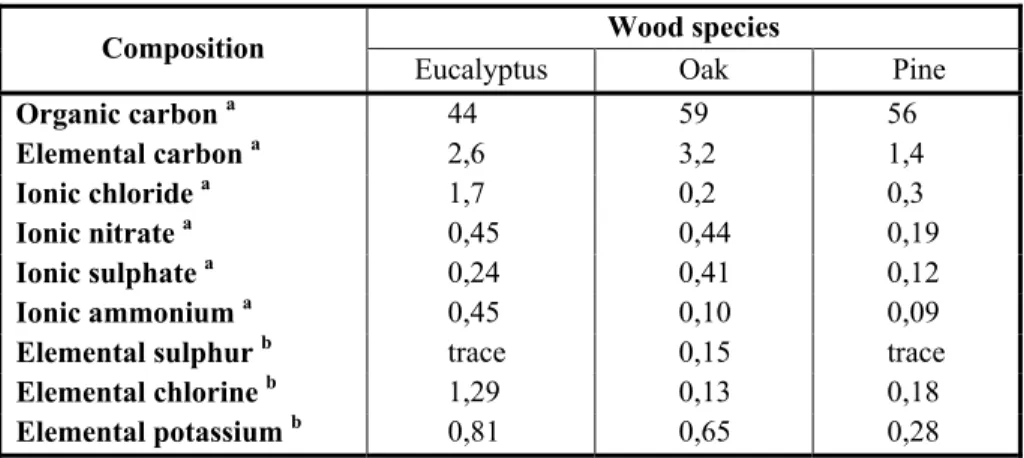
In a study carried out by Schauer et al. (2001) it was determined that the particle composition was dominated by organic compounds with a small amount of elemental carbon. Compositional analysis on three different wood species yielded results as shown in Table 1.1. The organic carbon content varied from 44% to 59% of total particle mass, in addition to 1% - 3% of elemental carbon. The main trace elements were potassium, chlorine and sulphur.
Table 1.1 Compositional analysis of PM from residential wood combustion for three wood species
Data from Schauer et al. (2001 p. 1719)
Composition Wood species
Eucalyptus Oak Pine
Organic carbon a 44 59 56 Elemental carbon a 2,6 3,2 1,4 Ionic chloride a 1,7 0,2 0,3 Ionic nitrate a 0,45 0,44 0,19 Ionic sulphate a 0,24 0,41 0,12 Ionic ammonium a 0,45 0,10 0,09
Elemental sulphur b trace 0,15 trace
Elemental chlorine b 1,29 0,13 0,18
Elemental potassium b 0,81 0,65 0,28
a - measured as percentage of PM mass
b - measured by X-ray fluorescence as percentage of PM mass
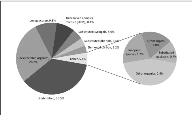
Approximately 50% of the organic carbon content could be extracted and analysed by gas-chromatography and mass spectrometry (GC-MS) techniques. Since hardwood species are mostly used for heating in Quebec, we will focus on the data for oak only. In order to get a clearer picture of the PM composition, the data for oak were transformed into a pie chart of percentages of total PM mass, as seen in Figure 1.1. The main point of interest here is that most of the particulate mass is not explicitly identifiable, even using advanced analytical methods. Fully 36,5% of the PM mass is unidentified in addition to 28,2% of unextractable organics, and the authors of the study did not propose any possible species, except to say that they are highly branched and cyclic organic compounds when referring to the unresolved complex mixture (UCM). For PM produced by oak combustion, the main constituent of the identifiable organic carbon was levoglucosan (1,6-anhydro-β-D-glucose), at 9,8% of the total particulate mass.
Unidentified, 36.5% Unextractable organics,
28.2%
Levoglucosan, 9.8% mixture (UCM), 8.4%Unresolved complex
Substituted syringols, 4.9% Substituted phenols, 3.6% Elemental carbon, 3.2% Other organics, 2.4% Inorganic species, 1.2% Other sugars, 1.0% Substituted guaiacols, 0.7% Other, 5.4%
Figure 1.1 Constituents of PM from oak combustion, percentage of total PM mass. Data from Schauer et al. (2001, p. 1719-1721)
Chemical analyses performed by Johansson et al. (2003) on the inorganic fractions of submicron particles collected during residential wood combustion showed that the main constituent elements are potassium, sulphur, chlorine and oxygen, with small amounts of sodium, magnesium and zinc. In addition, they determined that the dominant alkali compound present in the particles was potassium sulphate (K2SO4, 69% mass fraction),
followed by potassium chloride (KCl, 24% mass fraction). They also found that the combustion of more herbaceous biomass, such as straw, hay or forest residue, resulted in the relative abundance of the alkali compounds in the particles being reversed (i.e. KCl dominant). Hence, the relative abundance of the constituent elements in the fuel determines the composition of the resulting PM.
For the purposes of our study, the most important physical property that must be determined is the particle mass density. A recent study by Coudray et al. (2009) used a scanning electron microscope to analyze particles produced by wood combustion in order to estimate their
12
mass density. They found that mass densities ranged between 1 100 and 3 000 kg/m3 for particles of sub-micron diameter. It is likely that the particles have a relatively low melting point, since that of a β-D-glucose is 423 K at standard pressure. Hence, the particles are likely to be in a liquid form on formation, and solidify as their temperature falls while travelling in the flue gas. As for the dielectric constant (εr) of the particles, it is only possible
to estimate a value based on the values of its known constituents. A value for the εr of
levoglucosan could not be found in any chemical or physical reference tables, but values for sucrose, which is also a sugar, were found to range from 1,5 to 3,3.
1.2.2 Experimental data from biomass combustion
Experimental evidence suggests that most particle size distribution curves fit a lognormal distribution. Details of the lognormal distribution can be found in Wark and Warner (1981). The experimental particle data can be plotted on a log-probability chart of cumulative percent less than stated size versus logarithm particle diameter and if the distribution is lognormal, this will result in a straight line. The particle diameter with a cumulative percent of 50% equals the Count Median Diameter (CMD), and is equivalent to the geometric mean diameter (dg) based on count. In a similar fashion, the geometric standard deviation (σg) can be
determined from the graph by measuring the diameter at the 84th percentile (d84%) and using
the following relation from Wark and Warner (1981):
% (1.1)
The CMD and σg together completely define the lognormal distribution, and another useful
property described by Wark and Warner (1981) is the fact that σg is constant for lognormal
distributions based on values other than number count, for example mass and volume distributions. This property enables us to easily convert from number to mass distributions for example, using the Hatch-Choate equations originally derived by Hatch and Choate (1929). In the above case, the conversion equation is as follows:
MMD CMD e( (1.2)
where MMD is the Mass Median Diameter, which is always greater than or equal to the CMD. Similar equations exist for conversion between CMD and various different diameters, such as the mean and modal diameters. In order to put the difference between the CMD and the MMD into perspective, consider that in a typical sample of atmospheric particulate, the particles in the size range 0-1 μm constitute only 3% of the total sample mass, but make up 99,99% of the number of particles, according to Wark and Warner (1981, p. 146).
Several experimental studies have been carried out to better characterize the emissions from wood burning stoves of different types, including residential and industrial scale appliances. Generally, these studies focus on the different chemical species produced during wood combustion, but also include some data on the PM emissions. In two separate studies carried out by Johansson et al. (2003) and Johansson et al. (2004) values for the CMD were found to be in the submicron range from 0,1 to 0,3 μm for a range of different types of wood burning appliances, including both old and modern wood stoves and pellet stoves. Hedberg et al. (2002) measured a MMD of 0,5 μm from burning birch wood logs in a commercial wood stove. Kleeman, Schauer and Cass (1999) measured particle mass distributions from burning several types of wood (pine, oak and eucalyptus) and found similar profiles with MMDs ranging from 0,1 to 0,2 μm. Finally, a study by Hueglin et al. (1997) measured the particle number distributions from three phases of wood burning and showed that the greatest emissions were during the start-up phase, with a CMD of 0,24 μm. The lowest emissions were during the intermediate phase, with a CMD of 0,16 μm. In summary, it is clear that there is wide scientific consensus that the PM emissions from wood combustion are mainly in the sub-micron range (diameters ranging from 0,1 to 1 μm).
Apart from the particle size distributions, it is also important to measure the particle emissions rate. The emissions rates are also influenced by many variables, as for the size distributions. The emissions rate determined from the study by Schauer et al. (2001) for oak combustion is 5,1±0,5 grams of PM emitted per kilogram of wood burned (g/kg). The study
14
by Hedberg et al. (2002) for the combustion of birch wood obtained an average emission rate of 1,3 g/kg. McDonald et al. (2000) obtained emission rates from 2,3 to 7,2 g/kgfor mixed hardwood and oak combustion in wood stoves under a range of operating conditions. Based on these results, an average emission rate for hardwoods is calculated as 4,0 g/kg. The average burn rate for these tests was calculated to be 4,6 kg/h. The average emission rate in terms of grams per hour is a more useful measure, and is calculated to be 15,7 g/h. It is interesting to note that this emissions rate is well above the maximum rate required for U.S EPA (1988) stove certification (7,5 g/h).
1.2.3 Particulate emissions control methods
Currently the most widely explored and applied means of reducing PM emissions from wood stoves focus on increasing the efficiency of the combustion process in the stove itself. The most popular methods for achieving this fall into two categories: catalytic and non-catalytic. The simplest method is non-catalytic, which achieves increased combustion efficiency through the addition of three modifications to the traditional wood stove. These are the addition of insulating bricks in the firebox, an increased baffle size, and the introduction of pre-heated secondary air into the top part of the firebox. Catalytic stoves on the other hand, have a more complex design based on the addition of a catalyst-coated structure through which the exhaust gases flow and burn much of the smoke, making them more efficient and hence less polluting than non-catalytic stoves. However, the catalytic stoves are significantly more expensive, and the catalyst unit degrades relatively quickly with time.
The main problem with the focus on improving combustion efficiency is that existing stoves cannot easily be retrofitted with the above technologies, and the existing stove must be replaced altogether. The province of Quebec now requires by law that new/replacement installations meet the U.S. EPA (1988) standard. Many wood stoves now on the market have certified emissions rates under 4,0 g/h, however the lifespan of a wood stove can be up to 30 years, so existing older and more polluting stoves will continue to be used and to pollute the air more than new stoves for many years to come.
Another important factor is that despite the technological advances in stove design mentioned above, the actual PM emissions produced depend on the user following the basic rules of wood burning. These are always provided in the user guide for new stoves, and the most important one according to the Canada Mortgage and Housing Corporation (2008) is to burn only well seasoned (dry) split hardwood. It is necessary to follow the operating instructions carefully, as incorrect operation can greatly increase PM emissions. However, it is human nature not to follow instructions, and one can conclude that in general the actual emissions from any given stove will be greater than those obtained under optimal conditions during certification (as evidenced by the experimental results mentioned in section 1.2.2).
Taking the above facts into consideration, it is clear that even the most advanced wood stove can be made to operate inefficiently through user misuse. Therefore, our hypothesis is that if an emissions control device could be installed downstream from the stove itself (at the chimney exit) emission rates could theoretically be controlled regardless of how the stove is operated. Existing installations could simply be retrofitted at the chimney exit and could in theory be applied to all existing stove installations regardless of type.
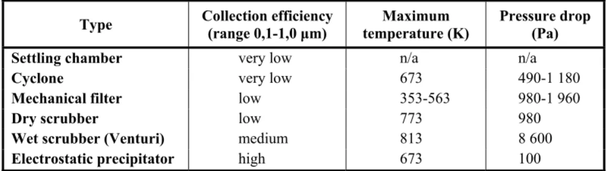
There are currently no known widely available commercial means for particulate emissions control downstream from residential wood stoves in North America. The main emissions control methods discussed in this section are listed in Table 1.2. They are all used by industry, most notably by coal-fired power stations and the cement manufacturing industry, where very large quantities of PM are produced and must be efficiently controlled to prevent widespread environmental problems. Most often, several different control devices are installed in combination. It must be noted that the scale of these control devices is also industrial, and much of the engineering challenge lies in reducing the scale of these devices to the residential scale while retaining their high collection efficiencies.
Mechanical filtration using closely spaced fibres to capture particles is the most common type of filtration for particle sampling. Modern filter designs are highly effective in certain applications. The wide range of different types of filter materials available, each with its own
16
characteristic properties and performance, are one of the reasons for their popularity. Industrial filtration takes the form of a so-called baghouse, large house-sized chambers containing the filter material.
Table 1.2 Summary table of emissions control devices and characteristics Adapted from Vallero (2008)
Type Collection efficiency (range 0,1-1,0 μm) temperature (K) Maximum Pressure drop (Pa)
Settling chamber very low n/a n/a
Cyclone very low 673 490-1 180
Mechanical filter low 353-563 980-1 960
Dry scrubber low 773 980
Wet scrubber (Venturi) medium 813 8 600
Electrostatic precipitator high 673 100
There are however several reasons why filtration is never used as the primary PM control device in coal fired utilities. Firstly, placing a filter into the flue gas flow creates an obstruction to the flow. This in turn causes a pressure drop on either side of the filter, which is proportional to the thickness of the filter. Pressure drop therefore restricts the flow, and if the pressure drop is greater than the normal pressure difference causing the flow, then the flow will be completely obstructed. For obvious reasons, this cannot be allowed to happen in a residential chimney, where the draft created during operation of the wood stove is quite small at less than 100 Pa for a standard residential chimney stack, as calculated using the formula by Perry and Green (1984).
Mechanical filters tend to clog up with use, causing an increase in pressure drop and a decrease in efficiency over time. Regular replacement of filters is normally required in industrial applications, making them unattractive options for residential use. Most common filters are unsuited for use in extreme conditions, such as those that exist in chimney stacks (high temperature, presence of corrosive chemical species, etc.). Therefore, the performance of filters in such conditions is likely to be unsatisfactory. Based on the above facts,
mechanical filtration is not deemed to be a suitable PM control device for residential applications.
Another common control device is the cyclone, which uses the principle of centrifugal separation of particles from the gas flow. Cyclones are systematically installed at coal-fired utilities, and they act as cost efficient pre-cleaners. In a cyclone, the dirty gas enters through a horizontal duct at the top of a vertical cylinder. The gas is forced into a helical downwards motion at first, forming a vortex, the particles are forced outwards to the cyclone walls through the centrifugal force and their own inertia. The particles slide down the walls and are collected at the bottom of the device. Detailed analyses of cyclone collection performance have been carried out in order to maximize their efficiencies. The main result presented by Wark and Warner (1981) is as follows:
(1.3)
where η is the collection efficiency, vp is the particle velocity, ρp is the particle mass density,
Rc is the cyclone radius and μg is the gas viscosity. The collection efficiency is proportional
to the square of the particle diameter so that efficiencies are low for small particles. A low inlet gas/particle velocity, as would be the case for a wood stove flue gas, means low cyclone collection efficiency. In addition, efficiency decreases with increasing gas viscosity, as is the case for high temperature flue gas. From this, it is clear that cyclones are not well suited to collect submicron particles, due mainly to the low inertia of such particles.
Next there are scrubbers, which are devices that pass the flue gases through some filtering medium, which can be solid or liquid, hence the terms wet or dry scrubber. According to the description by Vallero (2008), in a wet scrubber the particle-laden gas stream passes through a liquid spray in order to capture the particles in the liquid. The captured particles are then removed from the gas flow on a collecting surface, which can be a type of inertial collector. The dry scrubber passes the flue gas through a bed of solid matter, such as fine gravel, that is continuously re-circulated by an external mechanism. This matter acts as a filter, cleaning the
18
gas is a similar fashion, but without the problem of clogging. Both wet and dry scrubbers are large, complex devices, which require frequent maintenance and consume power and water (wet scrubber). It is clear that these devices are unsuitable for adaptation to a smaller scale for residential use.
As can be seen from Table 1.2, the electrostatic precipitator (ESP) is the only emissions control device able to capture submicron particles with high efficiency and a low pressure drop from a hot flue gas. It is for these reasons that ESPs have been in use for many decades in essentially all the worlds coal-fired utilities. Industrial ESPs have reached a high degree of sophistication in their design and operation, and they are also large and costly devices. Nonetheless, their operational characteristics mentioned above theoretically make them well suited for use in small scale residential applications.
1.2.4 Electrostatic precipitators
Electrostatic precipitators exist in a wide range of different geometries and scales, from tens of millimetres to tens of meters in size. Some devices are designed only to charge particles and not to capture them hence they have slightly different designs. But one thing they all have in common is a corona discharge region that generates an ion flux that subsequently charges the particles. The most common geometries are the wire-plate and the wire-cylinder.
According to Hinds (1999) in an industrial ESP the particle-laden flue gas is passed through a series of vertical metal collector plates. A high direct-current (DC) voltage is applied to thin vertical wires hung between pairs of grounded collector plates (a wire-plate geometry). The high voltage causes an intense non-uniform electrostatic field to be generated between the wire and plate. In the initial stage, the uncharged particles gain electrical charge through bombardment by ions generated in a thin corona discharge region surrounding the wires. The corona discharge region is essentially a highly ionised gas referred to as plasma. The corona discharge occurs when the electric field strength at the wire surface is above a critical value required to ionise the surrounding air. This creates a self sustaining avalanche of ions and
electrons, which then move with high velocity along the electric field lines towards their opposite polarity source or sink. In the case of a negative wire polarity, the electrons move out of the corona discharge region and attach themselves to electronegative gas (O2)
molecules in air to form high concentrations of negative ions. The particles then gain negative charge as they move through this negative ion flow. If the inner wire polarity is positive, then high concentrations of positive ions will flow to the grounded plate, and the resulting charge on the particles will be positive. This mechanism, first described by Pauthenier and Moreau-Hanot (1932), is known as field charging, and according to Hinds (1999) is the dominant charging mechanism for particles greater than 1 μm in diameter.
The ion generation mechanisms are actually quite complex and very different for positive and negative corona, and this is in itself an entire domain of research. However, for the purposes of this study, the above description is sufficient. All coronas generate ozone from oxygen in the air. Industrial ESPs are usually operated at negative potential since higher voltages can be attained, and hence higher efficiencies, however this results in increased ozone generation. According to Hinds (1999), negative corona produces about ten times as much ozone as positive corona. Obviously this is an important consideration, since ozone is itself a pollutant at low altitudes.
A second mechanism for particle charging in the presence of a unipolar ion flux such as that created by corona discharge is known as diffusion charging, as described by Fuchs (1947). Here, the particles become charged by random collisions with ions due to their Brownian motion. Again according to Hinds (1999), diffusion charging is the dominant mechanism for particles of diameter less than 0,2 μm and a transition zone exists between 0,2 and 1 μm, where both field and diffusion charging mechanisms are operating. Any model dealing with particles in the sub-micron size range must take both mechanisms into account. Creating a unified model for field and diffusion charging in the transition zone has been the subject of much research in this field. However, an analysis of particle charging models carried out by Lawless (1996) determined that a simple sum of charges approach to estimating the total charge on a particle in the transition zone resulted in values which were comparable with
20
experimental data obtained by Fjeld, Gauntt and McFarland (1983) and Kirsch and Zagnit'ko (1990), among others. The sum of charges model presented by Lawless provides a basis for calculating the total charge on a particle of a given diameter in the simulation. Readers are referred to Chapter 2 for more details of this model.
In the second phase, the charged particles are accelerated towards the collector plates by the electrostatic force on them. Bernstein and Crowe (1981) showed that the overall collection efficiency of the device depends on a number of parameters, including: the applied E-field, the particle charge, the gas flow properties and the collector geometry. Finally, the accumulated dust is removed by rapping the collector plates occasionally.
Most current research on ESPs is focussed on large-scale industrial cleaning devices for coal-fired utilities. Many different designs have been tested to try and maximise the collection efficiency and minimize operating cost. In a recent review of ESP research, Jaworek et al. (2007) noted that collection efficiencies reached a minimum (70-80%) in the transition zone between 0,1 and 1 μm. This is known as the penetration window, and is due to reduced charge and increasing mobility of the particle with a decrease in size. Hence finding ways to increase efficiencies in the transition zone is the goal of current and future research in industrial ESP design. The existence of this efficiency trough in the transition zone described above (where particle collection is particularly difficult) is of great importance for this study since, as we have seen in the preceding sections, the peak emission of wood combustion particles often lies in the transition zone, and these are the particles that can penetrate furthest into the alveolar region of the lung and have damaging health effects.
An experimental and theoretical study of small scale ESP performance in the ultra-fine and submicron size range was carried out by Zhuang et al. (2000), where they built and tested a wire-cylinder type ESP with a diameter of 0,03 m and length of 0,15 m. Artificial aerosols (including NaCl, SiO2 and Al2O3) were used to simulate particles at concentrations
comparable to emissions from wood combustion. They measured collection efficiency as a function of particle diameter and found that a maximum efficiency of 80% was reached at a
diameter of 0,085 μm for alumina particles under a given set of charging conditions and flow field parameters.
Only one experimental evaluation of a prototype ESP specifically designed for reducing PM emissions from residential heating appliances could be found in the literature, namely that by Schmatloch and Rauch (2005). This device was tested using emissions from a commercially available pellet boiler. A modified wire-cylinder geometry was used with a positive ionisation voltage of up to 20 kV, resulting in an overall collection efficiency of nearly 90% (by particle number) over a particle size range from 0,02 to 0,6 μm. The details of several important parameters were absent from the paper, including the gas flow velocity.
1.3 Simulation techniques
Experimental setups for PM measurement from wood stoves are often complex, requiring the use of a range of sophisticated sampling and measuring instruments that may not readily be available to researchers. Although numerical simulations cannot replace an experimental study, they do allow different models and parameters to be tested in a relatively short space of time and within a limited budget. The results can then be compared with experiment to assess the validity of the simulation model. Once it has been shown to agree with experiment with some degree of accuracy, it can be used to simulate any number of different setups.
In order to get a good understanding of the operation of an ESP, it is necessary to understand the physical mechanisms at work in the device. The theory is relatively straightforward for particle motion in a vacuum, but is more complicated when we model a real-world situation, such as a particle moving in a turbulent gas flow. Simulation techniques in such situations are limited to numerical techniques that make use of the speed and memory of modern computers. The field of CFD has grown in parallel with the development of the microprocessor, and has become the standard for modeling in the scientific and engineering fields.
22
1.3.1 Computational Fluid Dynamics overview
The field of fluid dynamics is based on the following three fundamental physical principles:
A. Conservation of mass (continuity equation) B. Conservation of energy (energy equation)
C. Conservation of momentum (momentum equation)
The set of equations describing these principles are known as the Navier-Stokes (N-S) equations, the details of which can be found in any book on fluid dynamics, such as that by Hughes and Brighton (1999). These equations are non-linear partial differential equations (PDE), which cannot be solved analytically for most real-world problems. This problem is solved through the use of CFD methods. Commercial CFD software packages are generally very versatile and user friendly and can be put to use on any number of problems and provides rapid results, without the need for major programming and intimate knowledge of the N-S equations involved.
The aim of CFD is to replace the N-S equations with numerical equivalents and use the power of the microprocessor to advance the numerical equivalents step by step in a series of iterations in time until a final numerical description (or solution) of the principal flow-field variables (velocity, pressure, turbulence, temperature, etc.) is obtained. Thus, any solution obtained using CFD is only an approximation, although it can be a very good approximation, depending on the desired precision. It is not the intention of this work to delve into the details of CFD and the reader is referred to Wendt (1995) for details on the basic theory.
1.3.2 CFD simulation of an ESP
Initial attempts to simulate the operation of an ESP using a CFD approach involved the use of numerical methods custom written for the purpose. For example Watanabe (1989) proposed a method for calculating individual fly-ash particle trajectories in a wire-plate ESP. Such custom methods lack the power and flexibility of a commercial CFD package, but
nonetheless produced a basic working model in general agreement with the experimental data. Since then, a number of similar simulations have been presented in the literature, with the more complete models using CFD numerical methods to calculate the turbulent gas flow field, the electric field, and the ion current including their effects on particle trajectories.
A simulation carried out by Choi and Fletcher (1997) made use of a commercial CFD package and took into account the effect of the particle space charge on the electric field and ion current. They concluded that in cases where there is a high mass loading of submicron charged particles, effects on the ion current and E-field distributions are significant and must not be neglected. The effect of a space charge is to restrict the ion current in the ESP resulting in a reduction in the collection efficiency. In a more recent simulation based on the above technique, Skodras et al. (2006) used a commercial CFD package to model an industrial wire-plate ESP over the particle size range 2 – 10 μm. It was found that collection efficiency for the smallest (2 μm) particles was less than 50%. They concluded that, for a given particle diameter, the inlet velocity and the electrical potential of the inner wire are the main factors that influence collection efficiency.
In summary, we will attempt to build a model and carry out a simulation based on the above works, and apply it to an ESP with a wire-cylinder geometry so that the collection efficiency of such a device may be modeled for particle sizes in the range 0,1 - 1,0 μm. This will in turn determine whether such a device is theoretically feasible for use in a residential installation.
CHAPTER 2 METHODOLOGY 2.1 The ESP model
This section will cover the theoretical details and steps involved in building the ESP model. Firstly, the physical basis for the ESP model will be established, followed by a description of the steps involved in applying CFD software to run the simulation and test the model. Finally, the assumptions and limitations of the model will be presented.
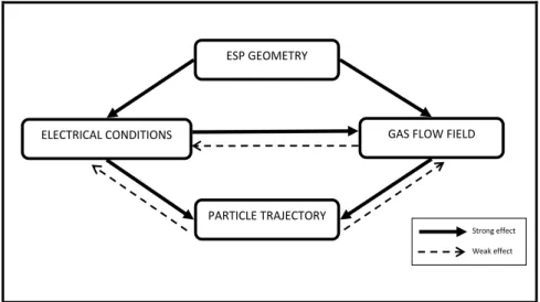
The construction of an ESP model requires an understanding of the processes at work, as well as their interactions. A schematic diagram showing the main processes and their interactions is shown in Figure 2.1.
Strong effect Weak effect
ESP GEOMETRY
GAS FLOW FIELD ELECTRICAL CONDITIONS
PARTICLE TRAJECTORY
Figure 2.1 Schematic diagram of the main components and interactions in an ESP.
Adapted from Schmid and Vogel (2003, p. 119)
As can be seen from Figure 2.1, there are three separate systems that mutually interact, or are coupled, namely the gas flow field, the electrostatic field and charge distribution, and finally the particle flow. What we are ultimately interested in is the individual particle trajectories,
but we cannot solve for this system in isolation of the other two systems if we wish to create a realistic simulation. Each of these three systems must be solved simultaneously since they are coupled, and in this way the different interactions are able to influence the overall solution process in a realistic way. Once the system has converged, it can be said that each system has reached its equilibrium (or steady) state, and the testing of collection efficiencies can proceed. The most effective means of creating such a model without spending an inordinate amount of time on programming is to use commercial simulation software. Since the model must account for the effects of gas flow through the flue pipe and the turbulence generated thereby, only software capable of modeling complex fluid dynamics problems should be used. The software deemed most fit for this purpose is FLUENT, by Fluent Inc. (2006a). The École de technologie supérieure is in possession of a license for this software.
2.1.1 Gas flow field
As mentioned in section 1.3.1, CFD involves the numerical solution of the N-S equations for a given geometry (in 2 or 3 dimensions) and set of initial/boundary conditions. The basic steady state mass continuity equation in the notation of Fluent (2006a) is given as
· ( (2.1)
Where ρ is the gas mass density (kg/m3), U is the gas velocity vector (m/s) and Sm is the mass
source term, usually equal to zero if there are no sources of mass in the volume under consideration.
If we assume the incompressible flow of a Newtonian fluid (as will be the case for this study), the steady state equation for the conservation of momentum as stated by Hughes and Brighton (1999) can be written as
26
where P is the static pressure (Pa), µ is the dynamic viscosity of the fluid (kg/m/s), and B is the sum of body forces per unit volume (N/m3), which, according to Choi and Fletcher (1997), for the case of an ESP can be written as
D (2.3)
where g is the gravitational acceleration (m/s2), F
D is the aerodynamic drag force (N/m3), ρion
is the ion charge density (C/m3) and E is the electrostatic field (N/C). The form of the equation that is solved by FLUENT will depend on the geometry of the system. For example, an axisymmetric geometry requires the addition of an extra term of the form (1/r) to the left hand side of equation 2.2.
The simplest interior (within solid boundaries) flow regime is laminar (plug) flow, where the velocity profile perpendicular to the main flow direction is constant. This simple, if unrealistic, type of flow was used before more sophisticated models were devised, and is useful in certain situations where no turbulence is expected. In most real-world situations however, the use of a turbulence model is required. The turbulence model employed for this study is the realizable k-epsilon (k-ε) model as described by Shih et al. (1995), which was designed to address the deficiencies in the standard k-ε model, and is fully integrated in the FLUENT software. The type of turbulence model chosen will also modify the form of the two equations au-dessus.
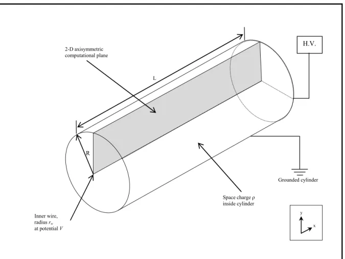
2.1.2 Electrostatics in a 2-D axisymmetric geometry
A commonly used ESP geometry is the wire-cylinder geometry shown in Figure 2.2, which has several practical and computational advantages, such as:
A. Cylindrical symmetry allows the use of a 2-D axisymmetric computational plane for modeling as shown by the shaded rectangular section in the figure;
C. Most residential wood stove flue pipes are cylindrical in shape.
Therefore, the simple wire-cylinder geometry presented here will be used as the reference case for the ESP model to be developed in the following chapters.
R Inner wire, radius rw at potential V L Space charge ρ inside cylinder Grounded cylinder H.V. 2-D axisymmetric computational plane y x
Figure 2.2 Schematic of the wire-cylinder geometry.
As described in section 1.2.4, corona discharge is initiated when the voltage applied to the inner wire exceeds a critical value. The empirical formula developed by Peek (1929) for a smooth, circular wire can be described as
28
where Ec is the critical value of the electric field at the wire surface (V/m), rw is the wire
radius (m) and δ is defined as
(2.5)
where To is the standard temperature (293 K) and p0 is the standard pressure (101 325 Pa), T
and P are the simulation temperature and pressure respectively. Since the current is zero at the critical voltage, the space charge in the cylinder is zero, and the equation for the electric field as a function of radius from the inner wire surface to the outer cylinder can easily be derived as shown by Hinds (1999)
( (2.6)
where V is the applied voltage at the wire (V), r is the radial distance from the wire surface (m), and R is the radius of the outer cylinder (m). This relation is only valid while there is no space charge present, i.e. the ion current is zero. The value of the critical wire voltage, known as the corona inception voltage (Vc) is then given by
(2.7)
Hence the thinner the inner wire, the greater Ec becomes, but a smaller value of Vc is required
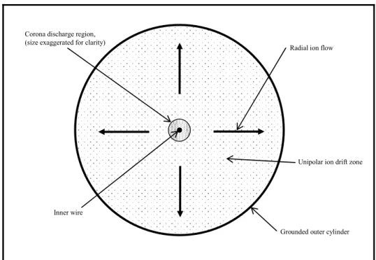
to initiate corona discharge. Once the wire voltage increases beyond the critical voltage, the corona discharge becomes established and an ion current begins to flow from the wire to the grounded collection cylinder. The presence of this ion space charge in turn affects the electrostatic field and an equilibrium condition is reached where there is (for negative wire voltage) an electrically neutral corona region near the wire, free electrons and negative ions in the space between the corona discharge region and the outer cylinder. A simple schematic of a cylindrical ESP is shown in Figure 2.3.