RESEARCH ARTICLE
Tropospheric Ozone Assessment Report: Present-day
distribution and trends of tropospheric ozone relevant
to climate and global atmospheric chemistry model
evaluation
A. Gaudel
1,2, O. R. Cooper
1,2, G. Ancellet
3, B. Barret
4, A. Boynard
3,5, J. P. Burrows
6,
C. Clerbaux
3, P.-F. Coheur
7, J. Cuesta
8, E. Cuevas
9, S. Doniki
7, G. Dufour
8, F. Ebojie
10,
G. Foret
8, O. Garcia
11, M. J. Granados-Muñoz
12,13, J. W. Hannigan
14, F. Hase
15,
B. Hassler
1,2,16, G. Huang
17, D. Hurtmans
7, D. Jaffe
18,19, N. Jones
20, P. Kalabokas
21,
B. Kerridge
22, S. Kulawik
23,24, B. Latter
22, T. Leblanc
12, E. Le Flochmoën
4, W. Lin
25,
J. Liu
26,27, X. Liu
17, E. Mahieu
27, A. McClure-Begley
1,2, J. L. Neu
23, M. Osman
29, M. Palm
6,
H. Petetin
4, I. Petropavlovskikh
1,2, R. Querel
28, N. Rahpoe
23, A. Rozanov
23,
M. G. Schultz
31,32, J. Schwab
33, R. Siddans
22, D. Smale
20, M. Steinbacher
34,
H. Tanimoto
35, D. W. Tarasick
36, V. Thouret
4, A. M. Thompson
37, T. Trickl
38,
E. Weatherhead
1,2, C. Wespes
39, H. M. Worden
40, C. Vigouroux
40, X. Xu
41,
G. Zeng
30, J. Ziemke
42The Tropospheric Ozone Assessment Report (TOAR) is an activity of the International Global Atmospheric Chemistry Project. This paper is a component of the report, focusing on the present-day distribution and trends of tropospheric ozone relevant to climate and global atmospheric chemistry model evaluation. Utilizing the TOAR surface ozone database, several figures present the global distribution and trends of daytime average ozone at 2702 non-urban monitoring sites, highlighting the regions and seasons of the world with the greatest ozone levels. Similarly, ozonesonde and commercial aircraft observations reveal ozone’s distribution throughout the depth of the free troposphere. Long-term surface observations are limited in their global spatial coverage, but data from remote locations indicate that ozone in the 21st
century is greater than during the 1970s and 1980s. While some remote sites and many sites in the heavily polluted regions of East Asia show ozone increases since 2000, many others show decreases and there is no clear global pattern for surface ozone changes since 2000. Two new satellite products provide detailed views of ozone in the lower troposphere across East Asia and Europe, revealing the full spatial extent of the spring and summer ozone enhancements across eastern China that cannot be assessed from limited surface observations. Sufficient data are now available (ozonesondes, satellite, aircraft) across the tropics from South America eastwards to the western Pacific Ocean, to indicate a likely tropospheric column ozone increase since the 1990s. The 2014–2016 mean tropospheric ozone burden (TOB) between 60˚N–60˚S from five satellite products is 300 Tg ± 4%. While this agreement is excellent, the products differ in their quantification of TOB trends and further work is required to reconcile the differences. Satellites can now estimate ozone’s global long-wave radiative effect, but evaluation is difficult due to limited in situ observations where the radiative effect is greatest.
Keywords: tropospheric ozone; ground-level ozone; Tropospheric composition and chemistry; Global tropospheric ozone burden; Ozone trends
1. Introduction
1.1. The Tropospheric Ozone Assessment Report (TOAR)
Tropospheric ozone is a greenhouse gas and pollutant detrimental to human health, and crop and ecosystem productivity (LRTAP Convention, 2015; REVIHAAP, 2013; US EPA, 2013; Monks et al., 2015). Since 1990 a large por-tion of the anthropogenic emissions that react in the atmosphere to produce ozone have shifted from North America and Europe to Asia (Granier et al., 2011; Cooper et al., 2014; Zhang et al., 2016). This rapid shift, coupled with limited monitoring in developing nations, has left scientists unable to answer the most basic questions: Which regions of the world have the greatest human and plant exposure to ozone pollution? Is ozone continuing to decline in nations with strong ozone precursor emissions
controls? To what extent is ozone increasing in the devel-oping world? Are natural sources of tropospheric ozone and its precursors changing? How can the atmospheric sciences community facilitate access to ozone metrics nec-essary for quantifying ozone’s impact on climate, human health and crop/ecosystem productivity?
To answer these questions the International Global Atmospheric Chemistry Project (IGAC) developed the
Tropospheric Ozone Assessment Report (TOAR): Global met-rics for climate change, human health and crop/ecosystem research (www.igacproject.org/activities/TOAR). Initiated
in 2014, TOAR’s mission is to provide the research com-munity with an up-to-date scientific assessment of trop-ospheric ozone’s global distribution and trends from the surface to the tropopause. TOAR’s primary goals are, 1) Produce the first tropospheric ozone assessment
1 Cooperative Institute for Research in Environmental Sciences,
University of Colorado, Boulder, US
2 NOAA Earth System Research Laboratory, Boulder,
Colorado, US
3 LATMOS/IPSL, UPMC Univ. Paris 06 Sorbonne Universités,
UVSQ, CNRS, Paris, FR
4 Laboratoire d’Aérologie, UMR 5560, CNRS and Université de
Toulouse, Toulouse, FR
5 SPASCIA, Ramonville Saint-Agne, 31520, FR 6 Institute of Environmental Physics, University of
Bremen, DE
7 Université libre de Bruxelles (ULB), Atmospheric
Spectroscopy, Service de Chimie Quantique et Photophysique, Brussels, BE
8 Laboratoire Inter-universitaire des Systèmes Atmosphériques
(LISA), UMR7583, Universités Paris-Est Créteil et Paris-Diderot, CNRS, Créteil, FR
9 Izaña Atmospheric Research Centre, AEMET, Santa Cruz de
Tenerife, ES
10 Laboratoire de Physico-Chimie de l’Atmosphère (LPCA), Maison
de la Recherche en Environnement Industriel 2 (MREI 2), Université du Littoral Côte d‘Opale, Dunkerque, FR
11 Izaña Atmospheric Research Centre (IARC), Agencia Estatal
de Meteorología (AEMET), Santa Cruz de Tenerife, ES
12 Table Mountain Facility, Jet Propulsion Laboratory, California
Institute of Technology, Wrightwood, California, US
13 Remote Sensing Laboratory (RSLAB), Department of Signal
Theory and Communications, Universitat Politècnica de Catalunya (UPC), Barcelona, 08034, ES
14 Atmospheric Chemistry, Observations & Modeling (ACOM),
National Center for Atmospheric Research (NCAR), Boulder, Colorado, US
15 Hase: Karlsruhe Institute of Technology (KIT), Institute
for Meteorology and Climate Research (IMK-ASF), Karlsruhe, DE
16 Deutsches Zentrum für Luft- und Raumfahrt, Institut für
Physik der Atmosphäre, Oberpfaffenhofen, DE
17 Harvard‐Smithsonian Center for Astrophysics, Cambridge,
Massachusetts, US
18 University of Washington Bothell, School of STEM, Bothell,
Washington, US
19 University of Washington Seattle, Department of Atmospheric
Sciences, Seattle, Washington, US
20 Centre for Atmospheric Chemistry, University of Wollongong,
Wollongong, AU
21 Academy of Athens, Research Center for Atmospheric Physics
and Climatology, Athens, GR
22 Rutherford Appleton Laboratory, Chilton, Didcot,
Oxfordshire, UK
23 Jet Propulsion Laboratory, California Institute of Technology,
Pasadena, California, US
24 BAER Institute, Mountain View, California, US
25 Meteorological Observation Center, China Meteorological
Administration, Beijing, CN
26 Department of Geography and Planning, University of
Toronto, CA
27 School of Atmospheric Sciences, Nanjing University,
Nanjing, CN
28 Institute of Astrophysics and Geophysics, University of Liège
(ULg), Liège, BE
29 Environment Canada/Cooperative Institute for Mesoscale
Meteorological Studies, The University of Oklahoma, and NOAA/National Severe Storms Laboratory, Norman, US
30 National Institute of Water and Atmospheric Research (NIWA),
Lauder, NZ
31 Institute for Energy and Climate Research – Troposphere
(IEK-8), Forschungszentrum Jülich, DE
32 Jülich Supercomputing Centre, Forschungszentrum Jülich,
Jülich, DE
33 Atmospheric Sciences Research Center, University at
Albany – State University of New York, Albany, New York, US
34 Empa, Swiss Federal Laboratories for Materials Science and
Technology, Duebendorf, CH
35 National Institute for Environmental Studies, Tsukuba, JP 36 Experimental Studies Research Division, MSC/Environment
and Climate Change Canada, Downsview, Ontario, CA
37 NASA/Goddard Space Flight Center, Greenbelt, Maryland, US 38 Karlsruher Institut für Technologie, IMK-IFU,
Garmisch-Parten-kirchen, DE
39 National Center for Atmospheric Research, Boulder,
Colorado, US
40 Royal Belgian Institute for Space Aeronomy, Bruxelles, BE 41 Institute of Atmospheric Composition, Chinese Academy of
Meteorological Sciences, China Meteorological Administration, Beijing, CN
42 Morgan State University, Baltimore, Maryland, US
Corresponding authors: A. Gaudel (audrey.gaudel@noaa.gov), O. R. Cooper (owen.r.cooper@noaa.gov)
report based on all available surface observations, the peer-reviewed literature and new analyses, and 2) Generate easily accessible and documented ozone exposure metrics at thousands of measurement sites around the world. Through the TOAR-Surface Ozone Database (https://join. fz-juelich.de, Schultz et al., 2017) these ozone metrics are freely accessible for research on the global-scale impact of ozone on climate, human health and crop/ecosystem productivity (TOAR-Surface Ozone Database, Schultz et al., 2017).
The assessment report is organized as a series of papers in a Special Feature of Elementa: Science of the Anthropocene. Three of the papers focus on the global distribution and trends of ozone relevant to different aspects of tropo-spheric ozone impacts, utilizing a range of ozone metrics described in the companion paper, TOAR-Metrics (Lefohn et al., 2018). TOAR-Health (Fleming et al., 2018) and
TOAR-Vegetation (Mills et al., 2018) rely on ozone metrics
drawn exclusively from the TOAR-Surface Ozone Database (Schultz et al., 2017). These metrics are of interest to sci-entists and policy-makers who wish to explore the impacts of ozone on human health and vegetation, impacts which typically occur during the warm spring and summer months. In contrast, this paper (hereinafter referred to as
TOAR-Climate) presents seasonal surface ozone metrics
that are designed to understand mean changes of ozone around the world, and that are appropriate for evaluating the global atmospheric chemistry models that calculate ozone’s radiative forcing (Stevenson et al., 2013). In addi-tion, TOAR-Climate summarizes ozone’s global distribu-tion and trends throughout the free troposphere using observations collected from ozonesondes, commercial air-craft, ground-based remote sensing instruments and sat-ellite instruments, and presents the first intercomparison of the global tropospheric ozone burden from multiple satellite instruments. TOAR-Climate focuses on the period from the mid-1970s to the present when measurements from modern UV-absorption instruments are widely avail-able. Further insight on ozone levels around the world from the late 1800s to the early 1970s, when ozone obser-vations were much more limited and based on a variety of methods, is provided by TOAR-Observations (Tarasick et al., 2018). An assessment of the present-day capabilities of the global atmospheric chemistry models used to calcu-late tropospheric ozone’s radiative forcing is provided by
TOAR-Model Performance (Young et al., 2018).
1.2. Tropospheric ozone’s relevance to climate
Due to its relatively short lifetime, tropospheric ozone is considered a ‘near-term climate forcer’, a class of com-pounds whose impact on climate occurs primarily within the first decade after their emission (IPCC AR5: Myhre et al., 2013). The influence of tropospheric ozone on cli-mate is dependent on its radiative forcing (RF) which is the change in the Earth’s energy flux since 1750 (due to changes of tropospheric ozone). The quantity of ozone in the troposphere in 1750 is unknown because observations in those days did not exist. The earliest quantitative obser-vations only began in the late 1800s and even then these
measurements suffered from interferences from other trace gases (see TOAR-Observations, Tarasick et al., 2018). In the absence of observations, global atmospheric chem-istry models are relied upon to estimate ozone in 1750. Based on output from multiple models, tropospheric ozone’s global-average radiative forcing is estimated to be 0.40 ± 0.20 W m–2 (IPCC, 2013). The relatively large error
bars of ± 50% are due to uncertainties in the estimate of pre-industrial ozone levels (Forster et al., 2007; Gauss et al., 2006; Mickley et al., 2001; Young et al., 2013), and uncertainties in the present-day spatial distribution of tropospheric ozone (Gauss et al., 2003; Kiehl et al., 1999; Naik et al., 2005; Portmann et al., 1997; Stevenson et al., 2006; Wu et al., 2007). Ozone can also affect radiative forcing indirectly due to its impact on vegetation, carbon uptake (Sitch et al., 2007; Lombardozzi et al., 2015), and methane lifetime (West et al., 2007; Fiore et al., 2008).
Improvement to the estimate of ozone’s radiative forc-ing requires greater confidence in global atmospheric chemistry model estimates of the tropospheric ozone burden (TOB: the total mass of ozone in the troposphere, Tg) in pre-industrial times, plus an accurate observation-based quantification of the present-day TOB and its hori-zontal and vertical distribution. The vertical distribution is especially critical because the relative greenhouse effect of ozone is greatest in the tropical and sub-tropical upper troposphere (UT), a region with limited ozone observa-tions (Lacis et al., 1990; Forster and Shine, 1997; Berntsen et al., 1997; Worden et al., 2008, 2011; Gauss et al., 2003, 2006; Bowman et al., 2013; Stevenson et al., 2013; Kuai et al., 2017). Current global atmospheric chemistry mod-els vary in their estimates of the quantity of tropospheric ozone originating from the stratosphere or from in situ photochemistry (Wu et al., 2007), but agree that photo-chemistry is the dominant gross source, exceeding the flux from the stratosphere by factors of 7–15 (Young et al., 2013; Banerjee et al., 2016). Most (~90%) of the ozone pro-duced in the atmosphere is also destroyed through photo-chemical loss processes, with the remainder deposited to the surface, which on an annual basis is similar in magni-tude to the flux from the stratosphere. These same mod-els estimate that approximately 30% of the present-day TOB is attributable to human activity and that the average present-day tropospheric ozone lifetime is approximately 22 days (Young et al., 2013). Further details on the tropo-spheric ozone budget are described in the TOAR compan-ion paper by Archibald et al. (2018), hereinafter referred to as TOAR-Ozone Budget.
In addition to changes of ozone precursor emissions, the quantity and distribution of tropospheric ozone is affected by unforced, low-frequency climate variabil-ity and long-term anthropogenic climate change (Jacob and Winner, 2009; Fiore et al., 2015; Barnes et al., 2016). Unforced climate variability refers to cyclical meteorologi-cal and transport patterns that affect tropospheric ozone at a particular location by modulating the frequency of air masses that are either enhanced or depleted in ozone, or by modulating cloud cover or air mass stagnation events which impact ozone photochemical production and loss.
Examples include El Niño/Southern Oscillation (Ziemke et al., 2015), the North Atlantic Oscillation (Eckhardt et al., 2003), the Quasi-Biennial Oscillation (Neu et al., 2014), the Pacific-North American pattern (Lin et al., 2014), and the frequency of synoptic scale heat-waves and mid-lati-tude cyclones (Mickley et al., 2004; Leibensperger et al., 2008; Shen et al., 2017). While climate variability produces interannual variability of observed ozone levels, anthro-pogenic climate change can produce forced long-term ozone trends. Many studies have examined the impacts of anthropogenic climate change on future tropospheric ozone levels and future ozone precursor transport path-ways (Fiore et al., 2015 and references therein; Barnes et al., 2016; Shen et al., 2016; Doherty et al., 2017). The gen-eral ozone response in a warmer climate is an ozone reduc-tion within air masses transported over long distances, due to an increase in water vapor and a decrease in ozone lifetime, but an ozone increase near the surface in regions where heat waves and air mass stagnation allow ozone pre-cursors to accumulate. However, to elicit a strong ozone response in a future climate the simulations require rela-tively high global temperature increases associated with radiative forcings of 4.5 or 8.5 W m–2 and 50 to 100 years
of climate change. On shorter timescales surface ozone trends due to anthropogenic climate change are difficult to detect as 20-yr ozone trends driven by unforced climate variability can be as large as those caused by changes in precursor emissions or anthropogenic climate change (Barnes et al., 2016; Garcia-Menendez et al., 2017). The longest continuous UV-absorption ozone records began in the mid-1970s and since then global temperatures have risen by approximately 0.7°C (Blunden and Arndt, 2017; NASA: www.columbia.edu/~mhs119/Temperature). Given the limited temperature increase so far over the span of the longest continuous surface ozone records, definitive attribution of observed global scale ozone changes due to anthropogenic climate change will likely require several more years of observations.
Previous assessments of tropospheric ozone have pri-marily focused on the processes that control ozone on the regional and global scale, and these works serve as a series of milestones in the scientific community’s collective understanding of tropospheric ozone (National Research Council, 1992; Team N.S., 2000; Brasseur et al., 2003; The Royal Society, 2008; Monks et al., 2015). In contrast,
TOAR-Climate assesses ozone’s global distribution and trends
from the mid-1970s to 2016, with the goal of providing a wide range of in situ and remotely sensed ozone observa-tions for quantifying the present-day TOB and to evaluate the global atmospheric chemistry models that estimate pre-industrial and future-scenario tropospheric ozone. Accordingly, TOAR-Climate studies ozone variability meas-ured at surface sites, but focuses on remote or non-urban sites because they are more easily compared to relatively coarse-scale global atmospheric chemistry models and because they are more broadly representative of regional-scale ozone. TOAR-Climate also explores ozone in the free troposphere (defined as the layer between the atmos-pheric boundary layer and the tropopause) as well as ozone in the full tropospheric column to quantify TOB and
its vertical and horizontal distribution. Another unique aspect of TOAR-Climate is the intercomparison of several near-global ozone products derived from in situ observa-tions and remote sensing. Many of these products, such as TCO from the OMI and IASI satellite-borne instruments, are quite new (Payne et al., 2017, Wespes et al., 2017) and are expected to form a key component of an evolving global ozone observational network (Burrows et al., 2011; Bowman, 2013). TOAR’s emphasis on collaboration has provided an opportunity to compare these satellite prod-ucts for the first time. The purpose of the intercompari-son is to determine if the various products agree in their quantification of TOB, TCO or long-term trends. The most robust results can then be used for global atmospheric chemistry model evaluation as described in TOAR-Model
Performance (Young et al., 2018).
The results of TOAR-Climate are presented as follows. Ozone metrics and statistics have been selected for their relevance to understanding average tropospheric condi-tions and for evaluating the global atmospheric chemistry models used to estimate pre-industrial and future ozone levels. The observations are from a wide range of instru-ments implementing in situ (surface ozone analyzers, air-craft-based instruments and ozonesondes) and remotely sensed techniques (ground-based Umkehr and FTIR, lidar and satellite), and are described in Section 2 and Table 1. The present-day global distribution of ozone at the sur-face, in the free troposphere and in the full tropospheric column is presented in Section 3. Trends in these same regions are presented in Section 4, with time series begin-ning anywhere from the mid-1970s (where data are avail-able) to the year 2000, and extending through 2014, 2015 or 2016, depending on data availability. Finally, Section 5 discusses ozone trends or distributions in several regions of the world and describes how the datasets used in
TOAR-Climate can be accessed.
2. Method
2.1. Surface ozone metrics relevant to climate and global model evaluation
TOAR-Metrics (Lefohn et al., 2018) describes all of the
ozone metrics in the TOAR database. The metrics relevant to climate and global atmospheric chemistry model evalu-ation that were selected for TOAR-Climate are: 1) the sea-sonal daytime average (8:00 to 20:00 local time) for surface observations, 2) seasonal nighttime averages (20:00 to 8:00 local time) at mountaintop sites, 3) monthly and seasonal means for free tropospheric observations from commercial aircraft (IAGOS), ozonesondes and lidars, as well as for TCO retrievals from space and ground-based remote sensing instruments. In some instances 5th, 50th,
95th and 98th percentiles are also shown. The present-day
period is defined as the 5-years between 2010 and 2014. Seasonal ozone values at surface sites are assessed for 2010–2014, with each site required to have at least three years of data during this 5-year period, and data capture of at least 75% in any season (Schultz et al., 2017). At a given surface site the magnitude of the temporal ozone trend is determined with the Theil-Sen (T-S) estimator, and the significance of the trend is determined with the
Table 1: All products discussed in this paper. DOI: https://doi.org/10.1525/elementa.291.t1 Product name
and institution Horizontal resolu-tion of gridded products
Horizontal
coverage Vertical range(tropopause defini-tion) Temporal resolution/time of day Record length Satellite OMI/MLS
NASA GSFC 1° × 1.25° 60°S–60°N Surface to tropopause(WMO 2 K km–1
lapse-rate) Monthly/ Seasonal 13:45 2004–2016, continuing GOME & OMI
Smithsonian Astrophysical Observatory (SAO) 1° × 1.25° 60°S–60°N Surface to tropopause (WMO 2 K km–1 lapse-rate) Monthly/Seasonal OMI: 13:45 GOME: 10:30 GOME: 1995– 6/2003 OMI: 10/2004– 2015, continuing OMI-RAL Rutherford Appleton Laboratory (RAL)1
5° × 5° 60°S–60°N Surface to 450 hPa mole fraction and surface to tropopause column (WMO 2 K km–1 lapse rate)
Monthly/ Seasonal 13:45 1995–2016, continuing IASI-LISA LISA Averaged over 0.25° × 0.25° grids
Regional (Asia) Surface to 6 km and 6–12 km Seasonal 9: 30 2008–2014, continuing IASI+GOME-2
LISA 1° × 1° Regional (Europe, Asia) Surface to 3 km, and 3–9 km Monthly/Seasonal9:30 2009–2010 IASI – FORLI
Université Libre de Bruxelles and LATMOS/IPSL
Averaged over
5° × 5° grids 90°S–90°N Surface to tropopause(WMO 2 K km–1 lapse
rate)
Seasonal
9:30 2008–2016, continuing
IASI – SOFRID
CNRS 5° × 5° 80°S–80°N Surface to tropopause (WMO 2 K km–1 lapse
rate)
Seasonal
9:30 2008–2016, continuing SCIAMACHY Averaged over grids
1° × 1°, 2° × 2°, 5° × 5° 80°S–80°N Tropopause to 60 km (blended tropopause) Monthly 10:00 2002/08–2012/4 Ground-based instrument FTIR
NDACC Point location Various sites around the world Surface to 8 km a.s.l. in this analysis. Retriev-als to 45 km are Retriev-also possible
Monthly/Annual Earliest data from 1995, continuing
Umkehr
Umk04+stray light correction, NOAA processing
Point location Various sites
around the world Surface to 250 hPa Monthly/AnnualMorning and afternoon profiles, averaged profile during measure-ments between 70–90° SZA, lati-tude and season dependent time of measurements
Earliest data from 1956 at Arosa, Switzerland, continuing
TOST 5° × 5° 90°S–90°N Surface to tropopause
(WMO 2 K km–1 lapse rate)
Seasonal/Annual 2008–2012 IAGOS 5° × 5° and airport
location Various airport in the world surface to 12 km Hourly (over Frankfurt) /Monthly /Seasonal
1994–2013
Lidar Point location 2 sites (OHP-France, TMF-California USA)
3 to 14 km (OHP)
4 to 18 km (TMF) Seasonal 1991–2015 (OHP)1999–2014 (TMF)
TOAR surface ozone metrics
Point location 3136 non urban sites
sea level to mountain top
Seasonal Most sites: 2000–2014 Selected sites: 1973–2017
nonparametric Mann-Kendall (M-K) test, as described in
TOAR-Metrics (Lefohn et al., 2018). Statistical significance
is based on an α value of 0.05, and all trends are reported with 95% confidence intervals. For a site to qualify for the 2000–2014 trend analysis, it must have at least 12 years of data and not more than 2 years missing at either end of the interval. In addition, data capture must exceed 75% in any given season.
TOAR uses specific units when describing ozone vations and levels of exposure. When referencing an obser-vation in ambient air, TOAR follows World Meteorological Organization guidelines (Galbally et al., 2013) and uses the mole fraction of ozone in air, expressed in SI units of nmol mol–1. Under tropospheric conditions the nmol
mol–1 is indistinguishable from the volumetric mixing
ratio ppb. The same units are applied to any ozone sta-tistic, such as median or 95th percentile values. In
TOAR-Health (Fleming et al., 2018) and TOAR-Vegetation (Mills
et al., 2018), the volumetric mixing ratio, ppb is used for the ozone exposure metrics discussed in those papers to maintain consistency with the ozone human health and vegetation research communities.
When referring to a TCO value, TOAR uses the Dobson unit (DU), where 1 DU is the number of molecules of ozone per square centimeter required to create a layer of pure ozone 0.01 millimeters thick at standard tempera-ture and pressure (or 2.69 × 10¹⁶ ozone molecules cm–2).
The tropospheric column extends from the surface to the tropopause, which can be defined according to a variety of methods including temperature lapse rate, tempera-ture cold point (tropical tropopause), trace gas thresholds or thermodynamic properties such as isentropic poten-tial vorticity. The choice of tropopause definition varies between research groups and due to the differences in altitude between the various tropopause definitions, inde-pendently calculated TCO values for a given time and loca-tion can differ by several DU. Discrepancies in tropopause altitude are particularly common at mid-latitudes in the region of the subtropical jet stream (Bethan et al., 1996; Wirth, 2000; Rodriguez-Franco and Cuevas, 2013).
2.2. Regionally representative surface sites
The TOAR-Surface Ozone Database (Schultz et al., 2017) contains climate-relevant ozone metrics at hundreds of surface sites around the world, both urban and rural. For this analysis a subset of non-urban surface sites has been selected for the purposes of illustrating the spatial and temporal variability of regionally representative ozone around the globe and for straightforward comparison to global atmospheric chemistry models. Urban sites were not considered because in spatial terms they are not regionally representative and because the local emissions and photochemical and deposition processes are too small-scale to be resolved by global atmospheric chem-istry models, as described by TOAR-Model Performance (Young et al., 2018). Sites were classified as urban if they exceeded thresholds for human population and satellite-detected nighttime lights intensity (see TOAR-Surface
Ozone Database for a detailed description of the site
clas-sification algorithm, Schultz et al., 2017). This selection
algorithm was applied to objectively identify the most highly urbanized sites, with approximately one quarter of all sites in the database classified as urban. The non-urban sites considered in this paper include suburban sites as well as rural sites surrounded by heavily urbanized areas. At the other extreme, some of the sites are considered to be remote, either located in unpopulated coastal regions, on islands, on top of high mountains, or in low-elevation, land-locked areas remote from anthropogenic emissions.
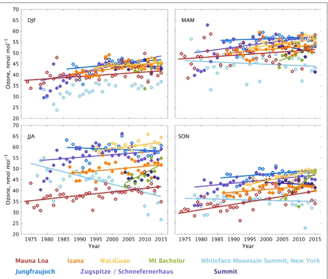
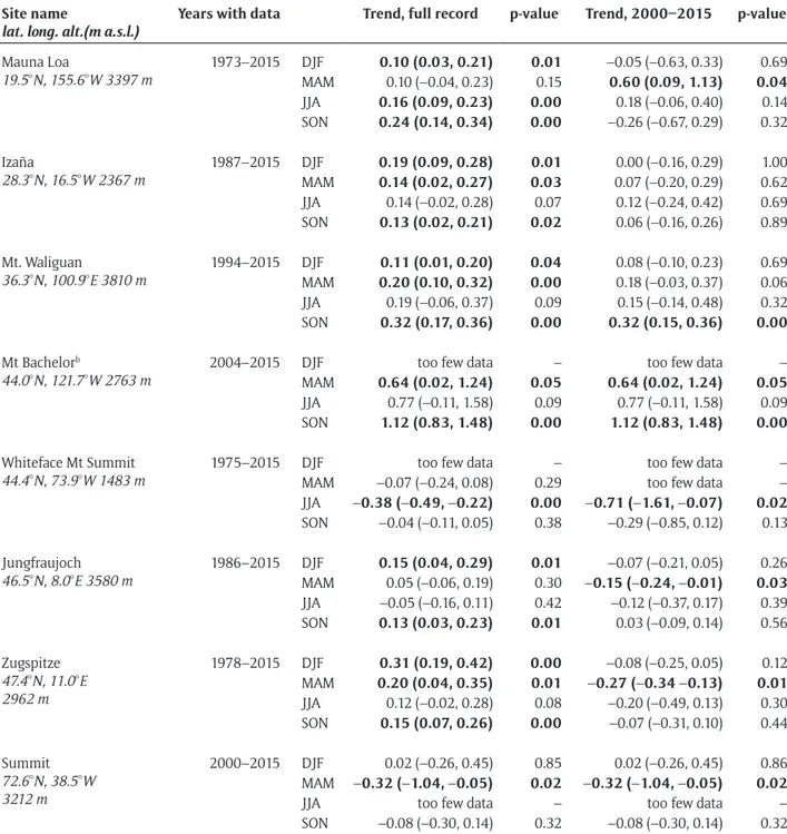
Another subset of sites was selected to explore long term trends in air masses characteristic of the lower free troposphere. This subset consists of eight mountaintop or very high elevation sites in the Northern Hemisphere. One of these sites, Mauna Loa Observatory (MLO) on the Big Island of Hawaii in the central North Pacific Ocean (19.5°N, 155.6°W, 3397 m), receives further analysis because of its location at the northern edge of the tropics. MLO is impacted by mid-latitude air masses which originate to the north and west and tropical air masses that originate to the south and east (Harris and Kahl, 1990; Oltmans et al., 2006). Ozone is typically greater in the mid-latitude air masses and the long term trend at MLO is affected by the relative frequency of air mass transport from high and low latitudes in response to climate variability driven by ENSO and the Pacific Decadal Oscillation (Lin et al., 2014). To reduce the noise in the trend due to climate variability we apply a new method for examining ozone trends at MLO (Ziemke and Cooper, 2017). Co-located dewpoint obser-vations are used to separate the ozone obserobser-vations into dry air samples, representative of mid-latitude air masses from higher altitudes and higher latitudes, and moist air samples, representative of tropical air masses from lower latitudes and lower altitudes. The dry/moist classification is performed for each month of the 1974–2016 time series using only nighttime data to avoid times with upslope winds. Each month must have at least 50% nighttime data availability. Dry air masses are those with a dewpoint value less than the monthly climatological 40th percentile, while
moist air masses are those with a dewpoint value greater than the monthly climatological 60th percentile. A dry or
moist category in any given month must have a sample size of at least 24 individual hourly nighttime observations. 2.3. Tropospheric ozone profiles: Ozonesondes, TOST, IAGOS, lidar
2.3.1. Ozonesondes
Ozonesondes are the most important source of verti-cally-resolved tropospheric ozone data for long-term cli-mate studies due to their very long record, with regular soundings beginning in the early 1960s (Hering, 1964; Hering and Borden, 1964, 1965, 1967; Komhyr and Sticksel, 1967a, b; Attmannspacher and Dütsch, 1970). Using KI-based electrochemical detection methods simi-lar to those developed for surface monitoring, they show good accuracy and reasonable stability over a 50-year period (Tanimoto et al., 2015; TOAR-Observations, Tarasick et al., 2018), and provide vertical resolution of about 100 m. Ozonesondes can be launched under cloudy conditions and therefore are not biased towards clear-sky conditions. Ozonesonde data are particularly valuable in the upper
troposphere-lower stratosphere (UTLS) region, especially in the tropics where much of the UT is not sampled by instrumented commercial aircraft. The UTLS is not highly-resolved by satellite instruments either.
However, ozonesonde data are temporally sparse and unevenly distributed, with only about 60 sites worldwide making regular soundings, most only once per week. Therefore TOAR-Climate uses a derived product that addresses these issues by taking advantage of the long lifetime of ozone in the free troposphere. This product is known as the Trajectory-mapped Ozonesonde dataset for the Stratosphere and Troposphere (TOST) and is described in Section 2.3.2. Ozone observations at individual ozone-sonde sites, for example, Lauder, New Zealand, are only assessed by TOAR-Climate for the purposes of evaluating remotely sensed TCO.
2.3.2. TOST
The Trajectory-mapped Ozonesonde dataset for the Strato-sphere and TropoStrato-sphere (TOST) is a 3-dimensional, long-term ozone dataset derived from ozone soundings using a trajectory-based ozone mapping methodology (Tarasick et al., 2010; Liu, G. et al., 2013; Liu, J. et al., 2013). TOST is derived from over 67,000 ozonesonde profiles at over 100 stations from the 1960s to 2010s. Locations of these sta-tions for the period 2008–2012 are shown in Figure S-1. The Hybrid Single-Particle Lagrangian Integrated Trajec-tory (HYSPLIT) model (Draxler and Hess, 1998), driven by the National Centers for Environmental Prediction (NCEP) reanalysis data, is applied to extend each ozone record along its trajectory path forward and backward for four days, as ozone lifetime in the free troposphere is a few weeks. Then, all ozone values along these trajectory paths are binned into grids of 5° × 5° × 1 km (latitude, longitude, and altitude), from sea level or ground level up to 26 km. TCO is integrated from the ozone concentrations below the tropopause, which is defined by the NCEP reanalysis data (Table 1). TOST provides a more accurate ozone dis-tribution than simple linear or polynomial interpolation of ozonesonde data. It depends on neither a priori data nor photochemical modeling and reveals ozone variations in three dimensions. It covers a longer term and higher latitudes than some satellite-derived tropospheric ozone data. TOST has been evaluated by comparing with indi-vidual ozonesondes (removed from TOST one by one). The agreement is generally quite good. Biases are larger near the tropopause, over mountainous regions and in areas with sparse soundings.
2.3.3. IAGOS
The In-Service Aircraft for the Global Observing System (IAGOS) program conducts long-term observations of atmospheric trace gases, aerosols and cloud particles on the global scale using commercial aircraft of internation-ally operating airlines. The origins of IAGOS lie with the MOZAIC (Measurements of OZone and water vapor on Airbus In-service airCraft) program, in which as many as five long-range Airbus A340 commercial aircraft provided in-situ measurements of ozone (as well as other species and thermodynamic parameters) along their flight routes
in various regions of the world (Marenco et al., 1998). Ini-tiated in August 1994, MOZAIC continuously measured tropospheric vertical profiles (landing and takeoff phase) and monitored the UTLS (cruise phase), until November 2014. Ozone measurements were performed using a dual-beam ultra violet (UV)-absorption monitor (time resolu-tion of 4 seconds) with an accuracy estimated at about ± (2 nmol mol–1 +2 %) (Thouret et al., 1998). As the
succes-sor to MOZAIC, with the objective of long-term sustainable operations, the first IAGOS aircraft became operational in July 2011 (Petzold et al., 2015; Nédélec et al., 2015). As of 2017, eight IAGOS aircraft from six airlines (Air France, Lufthansa, China Airlines, Cathay Pacific, Iberia and Hawaiian Airlines) are in operation. The 4-year overlap of MOZAIC and IAGOS has demonstrated that the new sys-tem provides data with the same quality as the former, per-mitting the reliable calculation of temporal trends from 1994 to the present (Nédélec et al., 2015). The MOZAIC-IAGOS data record (referred to as MOZAIC-IAGOS hereafter) now contains over 50,000 flights, freely available through the open-access central database (http://www.iagos.org). In this study, we use IAGOS data averaged in 5° × 5° grids in the UT and profiles over USA, Europe and Asia (Table 1).
2.3.4. Lidar
Differential Absorption Lidar (DIAL) is a well-known tech-nique to measure tropospheric and stratospheric ozone. The two DIAL systems described below contribute routine measurements 2–4 times per week to the Network for the Detection of Atmospheric Composition Change (NDACC).
The DIAL system located at the Observatoire de Haute Provence, France (OHP, 44°N, 6°E, 690 m) has operated since 1991 (Ancellet et al., 1997). The instrument measures ozone between 3 and 14 km above sea level (a.s.l.) with a vertical resolution ranging from 200 m at 2 km to 1000 m at 12 km. Precision remains within 9% at all altitudes, and accuracy is 5 ± 5 nmol mol–1. For this analysis, the
lidar data set is combined with data from Electrochemical Concentration Cell (ECC) ozonesondes launched weekly from OHP. Because the number of lidar profiles is 2 to 3 times higher than the number of ECC profiles, the combina-tion of both data sets improves the trend estimate obtained in the yearly ozone trend analysis (Gaudel et al., 2015).
The second DIAL used here is the tropospheric ozone lidar operated since 1999 at the Jet Propulsion Laboratory Table Mountain Facility in California (McDermid et al., 2002). The measurements cover altitudes between 4 and 18 km with an effective vertical resolution between 150 m and 3 km. Starting in 2006, the profile range was extended to 25 km by using a channel from a co-located water vapor lidar (Leblanc et al., 2012). The standard uncertainty is 5–10% throughout most of the profile, increasing to 15% at the top (Granados-Muñoz and Leblanc, 2016; Leblanc et al., 2016a).
2.4. Tropospheric Column Ozone from the ground 2.4.1. Ground-based FTIR
Observations from solar viewing ground-based Fourier Transform Infrared (FTIR) instruments are taken within the framework of the Network for the Detection of
Atmospheric Composition Change (NDACC, www.ndacc. org) and conform with the guidelines set by the Infrared Working Group (IRWG, https://www2.acom.ucar.edu/ irwg). They achieve a spectral resolution of 0.005 cm–1
or better. The ozone retrievals are performed using the 10µ spectral region and described in Vigouroux et al., 2015. Using the Optimal Estimation technique (Rodgers, 2000), up to 5 independent layers (or degrees of freedom of signal, DOFS) can be resolved to 45 km (see TOAR-
Observations, Tarasick et al., 2018). There is at least one
tropospheric layer (to 8 km a.s.l.), as defined as having DOFS of 0.8 to 1.0, depending on the station. This ozone partial column has expected random and systematic uncertainties of 11% and 4%, respectively (see
TOAR-Observations, Tarasick et al., 2018). The dominant
system-atic uncertainty are spectroscopic parameters. The total uncertainty is nominally 14%.
Among the NDACC FTIR stations, a subset provides time-series longer than 10 years (up to 23 years) for ozone trend studies (Vigouroux et al. 2008; García et al., 2012; Vigouroux et al., 2015; WMO, 2010; WMO, 2014). A list of the stations used in Climate is provided in
TOAR-Observations (Tarasick et al., 2018). The observations are
limited to clear sky daytime conditions, which excludes the polar night observations for the highest latitude stations. For all stations the average number of measurements is 2.5, 7, and 15 per day, week and month, respectively, but with high variability depending upon station location. 2.4.2. Umkehr Dobson and Brewer ozone profile retrievals Dobson (Dobson, 1968a, 1968b) and Brewer spectrome-ters (Kerr et al., 1981) are capable of ozone profile retriev-als from zenith sky measurements (so-called Umkehr curve method, Mateer, 1964; Mateer and DeLuisi, 1992; Petropavlovskikh et al., 2005). Details of the method and ozone uncertainties are discussed in TOAR-Observations (Tarasick et al., 2018). Tropospheric ozone variability cap-tured by the Umkehr method is determined by relative contributions of the a priori information and the measure-ment. The AK describes the mapping of the vertically dis-tributed sensitivity of the measurement into the retrieved ozone profile. Although the tropospheric Umkehr layer is defined between the surface and 250 hPa, a small but non-negligible contribution from the lower stratosphere has to be taken into account. Therefore, attribution of the lowest Umkehr layer information to TCO (below the trop-opause) variability is not well-defined and can be influ-enced by ozone variability in the lower stratosphere. The bias between Umkehr and other measurements, includ-ing ozonesondes and lidar has been identified (Komhyr et al, 1995; Fioletov et al., 2006; Nair et al., 2011). The bias between ozonesondes and Umkehr in the troposphere (~10–20%) is reduced by almost half when the ozone-sonde profiles are smoothed with the Umkehr AKs. Cor-rection for the out-of-band stray light error reduces the bias by about 5% (Petropavlovskikh et al., 2011), and the Umkehr tropospheric ozone data for this study are treated for stray light error (ftp://aftp.cmdl.noaa.gov/data/ozwv/ DobsonUmkehr/Stray%20light%20corrected/). The data have been deseasonalized prior to trend analysis.
2.5. Tropospheric Column Ozone from Space
TOAR-Climate provides an intercomparison of several
remotely sensed TCO products, as measured by satellite-borne instruments: OMI (Ozone Monitoring Instrument)/ MLS (Microwave Limb Sounder), GOME (Global Ozone Monitoring Experiment) and OMI-SOA (Smithsonian Astrophysical Observatory), OMI-RAL (Rutherford Apple-ton Laboratory), IASI (Infrared Atmospheric Sounding Interferometer)-FORLI (Fast Optimal Retrievals on Layers), IASI-SOFRID (SOftware for a Fast Retrieval of IASI Data), IASI-LISA (Laboratoire Interuniversitaire des Systèmes Atmosphériques), IASI+GOME-2, and SCIAMACHY (SCan-ning Imaging Absorption SpectroMeter for Atmospheric CHartographY). Details of each product are described below with key parameters listed in Tables 2 and 3.
As for ground-based remote sensing (section 2.4), sat-ellite data rely on retrieval algorithms that model the expected measured radiance with a forward model and then invert this model using the measurement, usually with optimal estimation (Rodgers et al., 2000), to pro-duce an estimated vertical distribution of abundance (nmol mol–1) or sub-columns (DU) along with a
posteri-ori error covariance and averaging kernel (AK) matrices. The AK quantifies the relative sensitivity of the radiance and retrieval to the “true state” for vertical retrieval layers and varies with observation type (land/ocean, day/night), the spectral range being measured (thermal infrared or UV), spectral resolution, measurement noise and choice of a priori covariance. For example, OMI/MLS, OMI-SOA, IASI-FORLI and IASI-SOFRID are more sensitive to the UT, while OMI-RAL is more sensitive to the lower half of the troposphere (Figures S-2, S-3 and S-4). In this report, we have taken care to use common parameters, where possible, such as tropopause height to determine TCO. However, fundamental differences remain due to the different measurement techniques and retrieval algo-rithms. Algorithm implementation details in addition to the choice of a priori, such as the choice of spectroscopic data and other forward model parameters can also have significant impacts on the retrievals, even for the same measurements using the same inversion technique (Liu et al., 2007; Liu et al., 2013). Finally, satellite ozone retrievals from various instruments differ due to sampling strategy, both spatially and diurnally (see Table 1).
2.5.1. OMI/MLS
Daily measurements of TCO and tropospheric ozone mean mole fraction were determined from the NASA Aura satel-lite’s OMI v8.5 total ozone (http://disc.sci.gsfc.nasa.gov/ Aura/data-holdings/OMI) and MLS v3.3 stratospheric column ozone (SCO) (Livesey et al., 2011). Calculation of TCO (Ziemke et al., 2006) requires subtraction of MLS SCO from OMI total ozone (TO) for near clear-sky scenes (OMI radiative cloud fractions less than 30%) yielding a 1° latitude × 1.25° longitude gridded product. SCO was first calculated along orbit paths using standard vertical pres-sure integration of MLS ozone mole fraction profiles from 0.0215 hPa to the tropopause pressure (determined from NCEP reanalyses using the WMO 2 K km–1 lapse-rate
hori-zontally (Gaussian + linear) between orbit paths to obtain gridded SCO fields at the 1° × 1.25° horizontal resolution of OMI, and then subtracted from the gridded OMI total ozone to derive daily gridded TCO fields.
Biases and long-term stability of OMI and MLS ozone measurements have been evaluated in detail (e.g. Hubert et al., 2016; Schenkeveld et al., 2016). OMI/MLS TCO calibration was tested here against ozonesondes and screened for cross-instrumental drift issues including the OMI row anomaly error (http://www.knmi.nl/omi/ research/product/rowanomaly-background.php). A small drift correction of –0.5 DU-decade–1 and a small offset
cor-rection of +2 DU was applied to this TCO product. The OMI/MLS tropospheric ozone mass burden calculated for 60°S–60°N was an average of 291 Tg in year 2004 and 306 Tg for 2016, a statistically significant net increase of about 5%.
2.5.2. GOME and OMI (SAO)
Ozone profiles with 24 layers (~2.5 km thick) from the sur-face to 60 km are retrieved from Global Ozone Monitoring Experiment (GOME; Burrows et al., 1999) and OMI (Levelt et al., 2006) radiances in the Hartley and Huggins bands using the optimal estimation technique (Liu et al., 2005, 2007, 2010; Huang et al., 2017). NCEP daily tropopause height based on the WMO 2 K km–1 lapse-rate definition
is used as one of the retrieval levels, allowing TCO, with its retrieval errors, to be derived from the retrieved pro-files. The time series from GOME (7/1995–6/2003) and OMI (10/2004–2015) are combined to produce a nearly 20-year record. GOME data prior to March 1996 are sys-tematically higher due to a shorter integration time and are not used in this study. To generate monthly GOME and OMI data to a common grid of 1° latitude × 1.25° longi-tude, only retrievals with good quality flags under near clear-sky conditions (with effective cloud fraction < 0.3) were used.
The individual retrieval TCO errors due to precision and smoothing errors are typically within 2–5 DU (14% on average), and average total errors including other system-atic and forward model errors are estimated to be ~21%. Both GOME and OMI TCOs typically show good agreement with ozonesonde TCO to within 3 DU. However, accurate radiometric calibration of Level 1b data as a function of time is critical to producing a long-term consistent data record. The degradation correction in GOME data might cause time-dependent systematic biases in the retrievals and no time-dependent correction is applied to OMI data even during the occurrence of the serious row anomaly since 2009. In addition, small GOME/OMI biases are expected due to some small algorithm differences and dif-ferent overpass times. As shown in Figure S-5, the time Table 2: Characteristics associated with IASI products used in this study. DOI: https://doi.org/10.1525/elementa.291.t2
IASI-SOFRID IASI-FORLI IASI-LISA IASI+GOME-2 (LISA)
Spectral range 1025–1075 cm–1 1025–1075 cm–1 7 wavelengths in
[975–1100 cm–1]
7 in [980–1070 cm–1]
2 in [290–345 nm]
RTMa SOFRID/
RTTOV FORLI KOPRA-KOPRAFIT KOPRAVLIDORT
Retrieval
method OEM
a OEMa Altitude dependent
TPa Altitude dependent TPa A priori Obs.a in 2008: Ozonesondes MOZAIC-IAGOS MLS
McPeters et al. (2007) McPeters et al.
(2007) McPeters et al. (2007)
Tropopause
Calculation Based on temperature profile from ECMWF analysis
(WMO thermal definitiona)
Based on IASI temperature from Eumetsat Level-2 products
(WMO thermal definitiona)
No use of tropopause
height estimation No use of tropopause height estimation
Vertical range Surface to tropopause Surface to tropopause surface to 6 km
6 to 12 km surface to 3 km
Cloud filter 20% 13% 15% 30%
Pressure level of peak of vertical sensitivity
500–400 hPa ~ 500 hPa 700–540 hPa 800–700 hPa
Reference Barret et al. (2011) Boynard et al. (2016,
2017), Hurtmans et al. (2012)
Dufour et al. (2012) Cuesta et al. (2013)
a RTM: Radiative Transfer Model; OEM: optimal estimation method; TP: Tikhonov-Philips; Obs.: Observations; WMO thermal
defini-tion: the thermal tropopause is defined as the lowest level at which the lapse rate is 2K km–1 or less, provided also that the average
series of GOME and OMI retrievals show clear systematic biases as some similar temporal patterns occur for differ-ent latitude bands, even though the seasonal variations are expected to be different (Liu et al., 2005, 2007, 2010; Huang et al., 2017).
2.5.3. OMI-RAL
Global height-resolved ozone distributions spanning the stratosphere and troposphere are retrieved from satel-lite UV nadir sounders by the RAL’s optimal estimation scheme (Miles et al., 2015). Data sets spanning 1995–2016 are being produced from a series of five instruments for ESA’s Climate Change Initiative (CCI) and will be updated in coming years for the EU’s Copernicus Climate Change Service (C3S). RAL’s scheme was the first to demonstrate tropospheric sensitivity (Munro et al., 1998). This is achieved through a three-step approach: firstly, the strong wavelength dependence of ozone absorption in the
Hart-ley band (260–307 nm) is exploited in fitting the ratio of backscattered to direct-sun spectra to retrieve height-resolved information principally in the stratosphere; secondly, an effective surface albedo is retrieved in the 335–340 nm interval and, thirdly, temperature depend-ent ozone absorption in the Huggins bands (323–334 nm) is fitted to high precision (<0.1% RMS) to extend the profile retrieval into the troposphere. Ozone prior infor-mation for the first step is from a zonal mean monthly climatology (McPeters et al., 2007). Retrieval outputs from the first and second steps improve the prior constraints for the third step. Precision on the 1013–450 hPa layer retrieved from an individual sounding is typically ~4 DU. This requires key instrument spectral and radiometric parameters to be pre-retrieved from direct-sun spectra and some instrumental and geophysical parameters to be co-retrieved with the ozone profile. The on-line forward-model is a modified version of GOMETRAN (Rozanov et Table 3: Characteristics associated with OMI and SCIAMACHY products used in this study. DOI: https://doi.org/10.1525/
elementa.291.t3
OMI/MLS GOME-OMI OMI-RAL SCIAMACHY
Spectral range OMI:
UV-1: 270–314 nm UV-2: 306–380 nm MLS: 240 GHz radiances GOME: 289–307 nm 325–340 nm OMI: 269–309 nm 312–330 nm UV-1: 266–307 nm UV-2: 323–336 nm 326–335 nm 264–675 nm
RTM TOMRAD VLIDORT Modified
GOME-TRAN++ SCIATRAN
Retrieval method LNMa OEMa OEMa LNMa
A priori Ozonesondes
SAGE/MLS
(McPeters et al., 2007)
McPeters et al. (2007) McPeters et al. (2007) Nadir: TOMS V7 ozone profile shape climatology (Wellemeyer et al., 1997)
Limb: Climatology generated with a chemical transport model (McLinden et al., 2000)
Tropopause
Calculation Based on temperature from NCEP Reanalysis (WMO thermal definitiona)
Based on temperature from NCEP Reanalysis (WMO thermal definitiona)
Based on tempera-ture from ERA-Interim Reanalysis (WMO thermal defi-nitiona)
Based on temperature and potential vorticity from ECMWF reanalysis, ERA-Interim (Both WMO thermal and dynamical definitiona)
Vertical range Surface to tropopause Surface to tropopause Surface to tropopause Surface to tropopause
Cloud filter 30% 30% 20% 30%
Pressure level of peak of vertical sensitivity
~500–300 hPa ~600 hPa ~800 hPa
Reference Ziemke et al. (2006) Liu et al. (2005, 2007,
2010)
Huang et al. (2017)
Miles et al. (2015) Ebojie et al. (2014)
aRTM: Radiative Transfer Model; OEM: optimal estimation method; LNM: Limb-Nadir-Match; WMO thermal definition: the thermal
tropopause is defined as the lowest level at which the lapse rate is 2K km–1 or less, provided also that the average lapse rate
between this level and all higher levels within 2 km does not exceed 2K km–1 (WMO, 1957); Dynamical definition: the dynamical
tropopause is characterized by a sharp gradient in potential vorticity (PV). The value used in the paper to define the tropopause is for PV = 2 pvu.
al., 1997). Developments since Miles et al. (2015) include: height-dependent treatment of rotational Raman scat-tering in ozone absorption lines and modifications for OMI’s 2-D detector array in place of across-track scanning by GOME-class sensors. Spectral coverage in the Huggins bands has also been extended to 321.5–334 nm. Develop-ments are in progress to improve near-surface sensitivity through addition of the ozone visible band (Chappuis) and, for GOME-2 on Metop, improvement of UTLS verti-cal resolution by addition of co-located IR measurements by IASI. The scheme as adapted for OMI will be applied to Sentinel-5 Precursor, launched in 2017, and subsequently to Sentinel-5 on Eumetsat’s Metop-SG series, planned for 2021–40.
2.5.4. IASI
IASI is a nadir viewing Fourier transform spectrometer that sounds the Earth-atmosphere system in the ther-mal infrared region. It operates from the Metop satellite series (Metop-A launched in 2006 and Metop-B launched in 2012) and provides global distributions twice a day for numerous trace gases (e.g. Clerbaux et al., 2009; Hilton et al., 2012). Four IASI ozone products are described below.
IASI-FORLI: Ozone vertical profiles are retrieved on the global scale in near real time with the FORLI-O3 (for IASI– v20151001) processing chain set up by the Université Libre de Bruxelles (U.L.B.) and LATMOS teams (Hurtmans et al., 2012). FORLI-O3 relies on a fast radiative transfer and on the optimal estimation method and provides profiles on a uniform 1 km vertical grid on 41 layers from the sur-face. FORLI-O3 uses only one single a priori profile and variance-covariance matrix which are built from a clima-tology. The code is implemented in the Eumetsat ground-based facility to become the official IASI ozone product to be distributed by Eumetcast in 2017. The FORLI-O3 product has undergone a series of validations against independent measurements (e.g. Boynard et al., 2018). The sensitivity of IASI in the troposphere maximizes around 4–8 km for most scenes. Negative ozone trends in the troposphere at mid-high northern latitudes have been reported, especially in summer (Wespes et al., 2018). For the present study, the daily tropopause height used to generate the IASI-FORLI TCO dataset relies on the WMO definition applied to the IASI level 2 temperature profiles provided through the Eumetcast operational processing system (August et al., 2012). Only daytime and clear-sky measurements characterized by a good spectral fit have been considered. Similar to other products, the IASI data were mapped on a daily basis to a grid of 5° latitude × 5° longitude, and then averaged to produce seasonal and annual means.
IASI-SOFRID: SOFRID retrieves global ozone (Barret et al., 2011) and CO (De Wachter et al., 2012) profiles from IASI radiances. SOFRID is built on the RTTOV (Radiative Transfer for TOVS) operational radiative transfer model (Saunders et al., 1999, Matricardi et al., 2004) jointly developed by ECMWF, Meteo-France, UKMO and KNMI within the NWPSAF. The RTTOV regression coefficients are based on line-by-line computations performed using the HITRAN2004 spectroscopic database (Rothman et al.,
2005) and the land surface emissivity is computed with the RTTOV UW-IRemis module (Borbas et al., 2010). We use the IASI-L2 temperature profiles from EUMETSAT for radiative transfer computation. The retrievals are per-formed with the UKMO 1D-Var algorithm (Pavelin, et al., 2008) based on the optimal estimation method (Rodgers, 2000). The results presented here are based on the IASI-SOFRID v1.5 ozone product (Barret et al., 2011). In this data version, SOFRID uses a single a priori ozone profile and associated covariance matrix based on one year (2008) of ozonesondes from the WOUDC network. The retrievals are performed for clear-sky conditions (cloud cover frac-tion < 20%). IASI-SOFRID ozone retrievals enable almost independent retrievals in the lower-middle troposphere (below 225 hPa), the UTLS (225–70 hPa) and the strato-sphere (above 70 hPa) (Barret et al., 2011). Dufour et al. (2012) have shown that IASI-SOFRID ozone tropospheric columns were in good agreement with coincident ozone columns from ozonesondes for the year 2008, with cor-relation coefficient of 0.82 (0.93) and 4 ± 4% at mid-lati-tudes and 5 ± 3% in the tropics.
IASI-LISA: The retrieval of the IASI-LISA ozone vertical profiles is performed using the radiative transfer model KOPRA (Karlsruhe Optimised and Precise Radiative trans-fer Algorithm), its inversion module KOPRAFIT, and a Tikhonov-Phillips (TP) altitude-dependent regularization (Eremenko et al., 2008). The retrieval constraints are opti-mized to enhance sensitivity in the lower troposphere (Dufour et al., 2012). Three different a priori profiles and constraint matrices are used depending on the tropopause height (for polar, midlatitude and tropical situations; see Dufour et al., 2015). Two semi-independent partial col-umns of ozone can be determined between the surface and 12 km (especially in the case of positive thermal con-trasts): the lower-tropospheric column, integrating the ozone profile from the surface to 6 km a.s.l.; the upper-tropospheric column, integrating the ozone profile from 6–12 km a.s.l. (Dufour et al., 2010, 2012). The lower-tropo-spheric column has a maximum sensitivity between 3 and 4 km with a limited sensitivity at the surface (Dufour et al., 2012). The retrieval algorithm is not optimized to provide near-real-time global data, and at present only regional data above Europe and Asia are available. For this study, only morning observations for clear-sky conditions (cloud fraction less than 15%) and high-quality pixels (based on quality flags) are used. The IASI-LISA product was mapped on a daily basis to a grid of 0.25° latitude × 0.25° longi-tude, and then averaged to produce seasonal means over the 2008–2014 period.
IASI+GOME-2 (LISA): In order to better characterize the vertical distribution of tropospheric ozone down to the lowermost troposphere (LMT, surface to 3 km a.s.l.), a new multispectral approach called IASI+GOME-2 combines the information provided by thermal IR radiances measured by the IASI instrument and Earth reflectance UV spectra from GOME-2 (Cuesta et al., 2013). Both co-located spectra are fitted simultaneously for deriving vertical profiles of ozone (for effective cloud cover < 0.3), providing multi-spectral retrievals at the IASI horizontal resolution (12-km diameter pixels spaced by 25 km at nadir). Both IASI and
GOME-2 are onboard the Metop satellites and they offer scanning capabilities with daily global coverage. Altitude-dependent Tikhonov–Phillips-type constraints optimize sensitivity in the lowermost troposphere, which exhibits a relative maximum around 2 to 2.5 km a.s.l. over land (where thermal contrast is positive). Further details are provided in TOAR-Observations (Tarasick et al., 2018). The multispectral synergism of IASI and GOME-2 enhances the vertical resolution of the retrieval so as to consistently resolve ozone levels in the lower/middle troposphere, the middle/upper troposphere and lower stratosphere. Since January 2017, global scale IASI+GOME-2 observations are routinely produced at the ESPRI French National data center (http://cds-espri.ipsl.fr) of the AERIS data center (http://www.aeris-data.fr) and will be available soon for the scientific community. For the current paper, the new capability of the recent IASI+GOME2 product is illustrated with the dataset available before 2017 (the year 2010 for East Asia and August 2009 for Europe).
2.5.5. SCIAMACHY
SCIAMACHY is a passive UV-Vis-NIR-SWIR spectrom-eter operated on board the European Envisat satellite from March 2002 to April 2012 (Burrows et al., 1995; Bovensmann et al., 1999). The instrument alternated between limb and nadir geometries so that the region probed during the limb scan was observed about 7 min-utes later during the nadir scan. TOCs are retrieved apply-ing the Limb-Nadir-Matchapply-ing (LNM) technique (Ebojie et al., 2014; Ebojie, 2014; Jia et al., 2017) to coincident limb and nadir measurements from SCIAMACHY. Thereby, the total ozone columns are derived from nadir observations while the limb measurements are used to retrieve strato-spheric ozone profiles. The latter are integrated down to the tropopause to obtain stratospheric ozone columns. TCO is calculated by subtracting the stratospheric ozone columns from its total column. The tropopause height was determined from the ECMWF ERA-Interim reanalysis, using a blended definition that transitions from a ther-mal tropopause definition in the tropics to a potential vorticity definition in the extra-tropics (Hoinke, 1998; Wilcox et al., 2012). As the lowermost altitude of the stratospheric O3 profiles used in this study (V2.9) is 12 km, extrapolation using ozonesonde climatologies was performed where needed. Only cloud free limb scenes and nadir pixels with cloud fraction < 30% were used. The analysis was restricted to solar zenith angles smaller than 80° and to the descending part of the orbit. The total error of the TCO data is estimated to be about 5 DU and is dominated by the error of the stratospheric ozone column.
2.6. Satellite observations of tropospheric ozone as a greenhouse gas
TES (Tropospheric Emission Spectrometer) operated on the NASA EOS-Aura satellite from 2004 to 2018 and measured vertical ozone profiles using thermal infrared spectra, similar to IASI, using Fourier Transform Spectrom-etry (Beer et al., 2001). TES obtained global observations
from 2004 to 2009 but shifted to a smaller latitude range following instrument failures associated with continu-ous operation. Seasonal mean TCO as measured by TES is shown for the years 2004–2008 in Figure S-6. Since IASI observations will continue into the next decade with identical IASI instruments on Metop-B and -C, there have been efforts to combine the TES and IASI data records by accounting for differences in spatial coverage, spectral resolution, and a priori information in the optimal esti-mation retrievals (Oetjen et al., 2014, 2016).
Radiative forcing due to tropospheric ozone has sig-nificant regional variability (Shindell and Faluvegi, 2009). While satellite observations cannot measure pre-indus-trial to present-day radiative forcing of tropospheric ozone, they can measure the ozone greenhouse effect of reduced TOA flux due to ozone radiance absorption. Long-wave (thermal infrared) measurements from TES and IASI are used to compute instantaneous radiative kernels (IRK) for ozone in W m–2 per nmol mol–1 for each vertical
pres-sure level. IRKs are computed along with the retrieved ozone vertical profiles using the Jacobians, K, which
quantify the sensitivity of the TOA radiance to each verti-cal profile (Worden et al., 2008, 2011; Doniki et al., 2015). Multiplying the IRK by the tropospheric ozone profile and summing the values from the surface to the tropopause gives the long-wave radiative effect (LWRE) in W m–2.
3. Present-day distribution of tropospheric ozone
3.1. Surface ozone
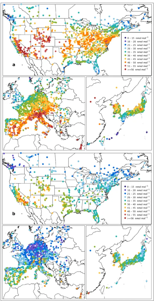
Non-urban surface ozone observations for the present-day (2010–2014) are mostly found in North America, Europe and East Asia (Korea and Japan); observations beyond these regions are relatively sparse. Figure 1 shows daytime average surface ozone mole fractions at all available non-urban sites in December–January–February (DJF) and in June–July–August (JJA), the minimum and maximum sea-sons of ozone production in the NH mid-latitudes (note that many US sites only operate during April–September, hence the fewer number of sites in DJF). In NH winter (DJF) high ozone (>40 nmol mol–1) is mainly confined
to high elevation regions: western USA, Western Europe (Alps, Apennines and Pyrenees), central Japan, central China, Himalayas, Greenland, southern Algeria and Izaña (Canary Islands). Such high ozone values are less frequent at low elevations, limited to western Canada, southern California, northeastern Utah (in a region of intense oil and natural gas extraction (Oltmans et al., 2016)), Israel, islands in the Mediterranean Sea and island/coastal sites in the vicinity of South Korea, Japan, Hong Kong and Taiwan. During NH summer, high ozone values (>50 nmol mol–1) are concentrated in northern mid-latitudes
at both high and low elevations, primarily in the western USA, southern Europe, China, South Korea and Japan. Ozone in the SH is more difficult to assess due to the sparse data coverage. The available observations indicate that SH ozone is much lower than in the NH, with only one region (the high elevation Highveld of South Africa (Balashov et al., 2014)) exceeding 40 nmol mol–1. These
high ozone events occur in DJF, and also in September– October–November (SON), which is springtime and the peak ozone season in the SH.
Figures 2 and 3 focus on the three regions with dense sur-face networks (North America, Europe, East Asia) and show daytime averages for all four seasons. In each region, maximum ozone is observed in spring/summer and the minimum ozone
is observed in autumn/winter. Notably, maximum ozone values in southeastern China, South Korea and Japan occur in spring, not summer. However, ozone in the Beijing region peaks in sum-mer. Finally, to illustrate the distribution of extreme ozone val-ues, Figure S-7 shows 98th percentile ozone at all available sites
around the world (urban and non-urban) for the 6-month warm season (April–September in the NH, and October–March in the Figure 1: Present-day global daytime average ozone (nmol mol–1). Global daytime average ozone (nmol mol–1)
at 2702 non-urban surface sites in December–January–February (top) and 3136 non-urban sites in June–July–August ( bottom) for the present-day period, 2010–2014. DOI: https://doi.org/10.1525/elementa.291.f1
Figure 2: Present-day regional daytime average ozone (nmol mol–1). Regional daytime average ozone (nmol mol–1)
at all available non-urban surface sites for December–January–February (DJF, a), March–April–May (MAM, b) for the present-day period, 2010–2014. Panel (a) shows the same data as Figure 1 (top), but focuses on the three regions with dense surface networks. DOI: https://doi.org/10.1525/elementa.291.f2
Figure 3: Present-day regional daytime average ozone (nmol mol–1). As Figure 2 but for June–July–August (JJA, a) and September–October–November (SON, b). DOI: https://doi.org/10.1525/elementa.291.f3
SH). Greatest values in North America are found in California and Mexico City. Europe has a strong north-south gradient with highest values in northern Italy, Spain and Greece. On the east-ern edge of the Mediterranean a monitoring site at 1 km a.s.l. in the West Bank has ozone values as great as those found in the heavily urbanized regions of Europe. Across Asia very high ozone values (>80 nmol mol–1) are widespread (northern India,
eastern mainland China, Hong Kong, Taiwan, South Korea, and Japan) despite a limited number of monitoring sites.
3.2. Free tropospheric ozone
3.2.1. Global ozone distribution in the free troposphere from aircraft and ozonesondes
Figures 4 and 5 show seasonal mean ozone in the UT as measured by IAGOS commercial aircraft and aver-aged using the methodology developed by Thouret et al. (2006). Measurements are obtained from aircraft cruising altitude (9–12 km a.s.l.), and cover a large portion of the NH mid-latitudes and tropics, and some areas of the SH.
Figure 4: Seasonal mean ozone (nmol mol–1) as measured by IAGOS commercial aircraft and by ozonesondes (TOST). Mean ozone (nmol mol–1) at four levels in the free troposphere as measured by IAGOS commercial aircraft
(2009–2013) at 9–12 km (UT), but below the dynamical tropopause (top row), and from ozonesondes (ozonesonde data from 2008–2012 spatially interpolated by trajectory-mapping in TOST) at 7–9 km (2nd row), 5–7 km (3rd row) and 2–3 km (bottom row). White areas indicate no data. Data are displayed seasonally for December–January– February (DJF, left) and March–April–May (MAM, right). DOI: https://doi.org/10.1525/elementa.291.f4
In the extra-tropics (30°S–90°S and 30°N–90°N), the UT is considered to be a layer 15–75 hPa below the local tropo-pause, defined as the 2 pvu (pvu = potential vorticity units) potential vorticity surface extracted from the European Centre for Medium-Range Weather Forecasts (ECMWF) operational analyses and forecasts. In tropical regions (30°S–30°N), where the tropopause is typically above the aircraft cruising altitude, all observations above 8 km are assigned to the UT. Mean ozone is calculated on 5° × 5° cells containing at least 300 observations over the 2009– 2013 period.
The seasonal distributions of ozone in the UT show a summer maximum that coincides with the maximum photochemical activity in the NH. Clear seasonal varia-tions are highlighted in the northern extra-tropics, with maximum values (>100 nmol mol–1) occurring in boreal
summer, and minimum values in boreal winter (<60 nmol mol–1). This is consistent with the seasonal pattern
previously observed over Europe, eastern North America and the North Atlantic Ocean, based on 1994–2003 MOZAIC observations (Thouret et al., 2006). The highest ozone is observed over Eurasia (including the Middle East) Figure 5: Seasonal mean ozone (nmol mol–1) as measured by IAGOS commercial aircraft and by ozonesondes (TOST). As Figure 5 but for June–July–August (JJA, left) and September–October–November (SON, right). DOI: https://doi.org/10.1525/elementa.291.f5