An Ant Colony System
for Responsive Dynamic Vehicle Routing
M. Schyns
∗Abstract. We present an algorithm based on an Ant Colony System to deal with a broad range of Dynamic Capacitated Vehicle Routing Problems with Time Windows, (partial) Split Delivery and Heterogeneous fleets (DVRPTWSD). We address the important case of responsiveness. Responsiveness is defined here as completing a delivery as soon as possible, within the time window, such that the client or the vehicle may restart its activities. We develop an interactive solution to allow dispatchers to take new information into account in real-time. The algorithm and its parametrization were tested on real and artificial instances. We first illustrate our approach with a problem submitted by Liege Airport, the 8th biggest cargo airport in Europe. The goal is to develop a decision system to optimize the journey of the refueling trucks. We then consider some classical VRP benchmarks with extensions to the responsiveness context.
Keywords. DVRPTW, heuristics, ant colony system, airport application, responsive-ness criterion.
1
Introduction
The starting point of this work is a problem submitted by Liege Airport (LGG), the 8th largest cargo airport in Europe. The goal is to develop a decision system that is able to optimize the journey of the airport’s refueling trucks. The trucks must deliver a standardized product, fuel, to aircrafts during predefined time windows corresponding to a sub period of the time on the ground. There are different types of trucks, operating at different speeds, and some of them are not capable of adequately serving certain models of aircraft. As is sometimes currently done, a delivery may be split between several trucks under certain conditions.
In this paper, we give special attention to optimizing a responsiveness objective in a dynamic environment. Indeed, while minimizing traveled distance is a classical objective in Vehicle Routing Problems (VRP), the highest priority for an airport is to complete the deliveries as soon as possible, allowing the aircrafts to return to operations. Airline companies have to pay for the time spent by aircrafts on the ground. As a result, inactive aircrafts not only fail to make money, but cost a lot too. Furthermore, flights must satisfy strict schedules and any delays will lead to financial penalties. In the worst cases, take-off or landing slots may be lost so that the flight has to be rescheduled or canceled. Since unexpected events may occur at any time, there is a strong reason to not only perform all the jobs in the allowed time window, but as soon as possible. This responsiveness is also crucial for many production or service activities in different fields: express parcel deliveries, taxi services, Just in Time production, express repair services, medical care, petrol station replenishment, etc.
∗QuantOM, HEC Management School, University of Liege, Rue Louvrex 14 (N1), 4000 Li`ege, Belgium.
The second challenge in this area is the uncertain dynamic environment. An airport operates continuously seven days a week. There is no clear end of the planning horizon nor perfect time to start an optimization. Moreover, the airport environment is highly uncer-tain; flights could be delayed or canceled, for example due to the weather or a breakdown. Similarly, quantities for fuel deliveries are initially only expectations, which will need to be tuned at the last moment depending on the load and weather conditions. We develop an interactive solution to allow dispatchers to take new information into account in real-time.
Our goal is therefore to present an approach to dealing with a broad range of Dynamic Capacitated Vehicle Routing Problems with Time Windows, (partial) Split Delivery and Heterogeneous fleets, in which this airport refueling problem belongs. Finding the optimal solution for a real size vehicle routing problem remains a challenge. VRPs are complex combinatorial problems, known to be NP-Hard. It is why exact methods in the literature typically focus on well-defined categories with restricted sets of constraints. This work is unique in that it simultaneously takes into account all the previously mentioned constraints, using an ant colony approach. This metaheuristic had already been adapted and proved to be a good strategy for solving the standard VRP and some extensions. In this research, we took inspiration from Gambardella et al. (1999) for the Vehicle Routing Problem with Time Windows (VRPTW) and from Montemanni et al. (2005) for the added dynamic dimension. We illustrate our approach with a specific instance provided by Liege Airport. We also test our algorithm on sets of popular VRPTW benchmarks. We start from the work by Montemanni et al. (2005) and use the same VRPTW datasets in a dynamic context. We also perform experiments utilizing some Solomon’s benchmarks. We compare different dynamic strategies and the impact of the responsiveness criterion.
Section 2 provides a brief literature review. In section 3, the main components of the problem are described in further details. In section 4, a classical Ant Colony System (ACS) algorithm for solving VRPTW is briefly revisited. In section 5, our extensions for addressing responsiveness and richer problems are described. Next, section 6 contains various strategies for improving the quality of the results. The results for the Liege Airport case and for the other benchmarks are presented and commented on section 7. Finally, conclusions are drawn in the last section.
2
Literature review
The problem under consideration belongs to the family of Vehicle Routing Problems. These problems are of crucial importance in practice for logistic and supply chain management. They are also complex combinatorial problems, known to be NP-Hard, which have aroused the interest of researchers for decades. Laporte (Laporte, 1992, 2009) highlighted the main contributions since the first paper on this topic, written in 1959 by Dantzig and Ramser (Dantzig and Ramser, 1959). Finding the optimal solution for a real-world problem remains a challenge. The most common approach in the literature is therefore to focus on simplified problems dealing with specific constraints one at a time. At the opposite, the first contri-bution of our work is to simultaneously integrate a very large set of characteristics so as to allow companies to easily use our framework for real-life problems. More precisely, we have simultaneously integrated in our framework the constraints separately studied in the following VRP subfields: Capacitated VRP (CVRP), VRP with Time Windows (VRPTW) (see, e.g., Br¨aysy and Gendreau, 2005; Cordeau et al., 2002; Kallehauge et al., 2005), VRP
with heterogeneous fleet (see, e.g., Choi and Tcha, 2007; Seixas and Mendes, 2013), VRP with multi-trips and Split Deliveries (see, e.g.,Archetti and Speranza, 2012; Dror et al., 1994; Salani and Vacca, 2011). Other constraints for variations like VRP with Backhauls or with Pickup and Delivery, VRP with multi-depots, Dial-A-Ride Problems are not included in our approach, even if it would be a natural and possible extension.
A second contribution of our work is linked to the nature of data. One of our main concerns is the uncertain dynamic environment. Following Ghiani et al. (2003), VRPs may be classified along two dimensions: static versus dynamic and deterministic versus stochastic. A VRP is said to be static if its input data do not depend explicitly on time, otherwise it is dynamic. A VRP is deterministic if all input data are known when designing vehicle routes, otherwise it is stochastic. The deterministic static cases are the most studied. Dynamic stochastic problems, also called real-time problems are more complex and less studied. Our work belongs to this last category. In this context, uncertain data is revealed during the course of the operational day and new plans have to be computed or adjusted after the new information arrives. As stated in Giaglis et al. (2004), this approach is requested in practice. While an initial planning minimizing the risk is necessary, we need methods to respond to unforeseen events when they happen. It is only more recently that technology has allowed consideration of such applications. Indeed, real-time applications require a powerful information system, such as systems based on GPS, to locate the vehicles and to communicate with them. Repeatedly computing new solutions also requires powerful computers or systems of computers (parallel computing as in Ghiani et al., 2003) and state-of-the art algorithms. In our framework, we accept and immediately react to any unexpected events, without relying on probability distributions and without identifying beforehand sets of possible future, as would be typically done in static stochastic approaches. The dynamic dimension of our work was inspired by the work of Montemanni et al. (2005) and is adapted to include the reoptimization strategy proposed by Gendreau et al. (1999). Our work also departs from these two papers by the extensive list of constraints we consider. Moreover, we believe that our third and main contribution is to propose a new objective criterion, i.e. responsiveness, especially adapted in such dynamic contexts. To the best of our knowledge, this approach is new and original.
State of the art methods to exactly solve VRPs are very complex. They typically rely on branch-and-cut-and-price algorithms and route relaxations strategies (see Baldacci et al., 2012). Richer and medium-sized problems generally remain intractable or too lengthy to solve with exact methods. In this context, the development of heuristics is the tradi-tional and often only reasonable approach. Many strategies are described in the liter-ature (see, e.g., Archetti and Speranza, 2012; Br¨aysy and Gendreau, 2005; Laporte, 2009 for a description of methods and surveys). Tabu search is probably the most often cited method, either alone or to expedite exact methods. Many authors also tackle VRP vari-ants using ant colonies. Other papers rely on ad-hoc heuristics, adaptive large neighbor-hood search or genetic algorithms. Our fourth contribution is to analyze the performances of an Ant Colony System (ACS) approach. We selected this metaheuristic based on the promising results described in the literature for the standard VPRTW (Gambardella et al., 1999). Note that many of our developments could be adapted to other local search meth-ods. Ant Colony Optimization (ACO), as explained in Dorigo et al. (1996), is inspired by the collaborative behavior of naturally independent agents: ants. This algorithm has been modified to solve many different discrete optimization problems (Dorigo et al., 1999). In particular, ACO was applied to graph optimization problems including the Traveling
Salesman Problem (Dorigo and Gambardella, 1997), which can be seen as a VRP with only one vehicle. This leads to the ACS, an improved version of the ACO. The ACO algorithm is very flexible, and other characteristics such as time dependency, uncertainty, real-time conditions, backhauls, pickup and delivery, heterogeneous fleet or other improve-ments were introduced one at a time in the literature (Benslimane and Benadada, 2013; Bin et al., 2009; Donati et al., 2008; Gajpal and Abad, 2009; Gambardella et al., 2003, 1999; Montemanni et al., 2005; Reimann et al., 2004; Rizzoli et al., 2007). In this research, we took inspiration from Gambardella et al. (1999) for the ant framework.
3
Problem description
We present an approach to dealing with a broad range of Dynamic Capacitated Vehicle Routing Problems with Time Windows, (partial) Split Delivery and Heterogeneous fleets (DVRPTWSD). Formally, this problem can be represented by a digraph G = (N, A) where N = {D, 1, . . . , n} is the set of nodes and A = {(i, j)|i, j ∈ N, i 6= j} is the set of arcs. The nodes in N \ {D} denote the clients to serve and D represents the depot. For each customer i in N \ {D}, we have a positive quantity qi to be delivered within a particular time window
[ai, bi]. This is a hard time window within which the service must be entirely completed. This
is a strong constraint justified by the huge penalties encountered by the companies when these windows are not respected, such as in the context of the airports. Note, however, that this constraint is essentially restrictive at the upper bound bi. As usually accepted for
VRPTW, a vehicle is allowed to arrive in advance but has to wait until the beginning of the time windows to start the service. No penalty is incurred in this case. We consider a single depot D from which each vehicle starts and must return. We assume that there is no demand at D and that the depot is always open. For algorithmic reasons, the depot D is duplicated once for each vehicle. Distances between copies of the depot are set to zero. Let V = {1, . . . , v} be the set of vehicles, Dk with k ∈ V is the virtual copy of the depot from
which vehicle k starts. dij and tij represent respectively the distance and the travel time
along the arc (i, j) ∈ A. We assume that tij is directly proportional to dij and that each
vehicle travels at the same speed.
The fleet of vehicles V is heterogeneous. Each vehicle k ∈ V is characterized by a specific capacity Ck, a service operating time and an incompatibility list. The operating time for
serving client j with vehicle k is defined as ok
j = ck + vkqj, where ck is the constant time
required by vehicle k for setup and post-operations, and vk is the variable time required by
vehicle k to deliver one unit of product. The incompatibility list takes into account that some vehicles are not allowed or not appropriate to serve some clients. For example, in the case of an airport, some trucks are too big to serve some small types of aircraft or are prohibited from delivering fuel to some specific flights. We also make the assumption that the fleet of vehicles belongs to the fleet handler. The size of such a fleet cannot vary dynamically with respect to the demand, and reducing the number of trucks operating simultaneously does not have a strong impact on the cost structure. We therefore do not attempt to minimize the number of vehicles in use.
We are concerned by situations where the responsiveness is more critical than the dis-tance traveled. Responsiveness is defined here as completing a delivery as soon as possible, within the time window, such that the client or vehicle are able to operate again. Note that minimizing the arrival time within the time window is not the only way to improve
responsiveness. The duration of the service, depending on the vehicle, must also be taken into account. The global objective to minimize becomes R =Pjsj+ ok(j)j − aj where sj ≥ aj
is the start of service time for client j and where the superscript k(j) is used to express that a specific vehicle k is determined by the algorithm to serve client j. By definition, since the operating service time is a strictly positive value, so is R. A lower bound can be computed beforehand. This objective is in contrast to the cost function computed in traditional VRPs where the goal is to minimize the total distance T =P(i,j)∈Adijxij (or a related function).
In this last function, xij is a binary variable that indicates if arc (i, j) is traveled in the
solution. Note that, in our context, when two solutions with the same responsiveness are found, the one with the shortest distance T is preferred.
In the VRP with split deliveries, a single customer can be served by different vehicles. The basic case is one in which the quantities requested by the clients are larger than the capacity of the vehicles. This can also occur in certain specific situations when the overall cost is decreased by splitting the delivery. A typical case is when the remaining capacity of a vehicle at the end of its trip is no longer large enough to serve another client. Instead of sending this vehicle back to the depot with a positive remaining capacity, it may be beneficial to empty the vehicle by visiting a final client before sending another vehicle to complete, either totally or partially, the delivery. In the airport context, this is the usual technique. Following our approach, a split delivery can only occur when the remaining capacity is not large enough to serve an attractive client. This covers the basic case where the vehicle capacities are smaller than the demands. However, it excludes a split delivery between vehicles which would have been able to fully serve a client on their own. This last strategy is rarely optimal due to the travel costs and the fixed amount of time required for any service. Moreover, several vehicles may be banned from serving the same client simultaneously. Such operations are often prevented by infrastructure constraints such as a limited number of unloading docks or an aircraft with one tank and one main inlet.
Our problem is a multi-trip VRP. The planning horizon may be extremely long, or even infinite, while at the same time the fleet size is limited. The same vehicle must be allowed to replenish to start a new tour afterward, if needed. Each time a vehicle comes back to the depot, we automatically load it again at full capacity. The time required for reloading vehicle k follows a scheme similar to the one for serving the clients : ok
D = ckD+ vDk(Ck− rk).
Specific constant and variable times, ck
D and vkD, are allowed for the depot. The quantity to
load is the difference between the full capacity Ck and the remaining capacity rk at the end
of the previous tour. As soon as the replenishment is complete, the vehicle is again available. Note that this multi-trip possibility also implies that a split delivery could be performed by a single vehicle.
Finally, we consider a stochastic dynamic environment. Many companies operate con-tinuously seven days a week. It is therefore not possible to precisely determine the end or the beginning of the planning horizon. Moreover, the world is uncertain: delivery quanti-ties might only be based on expectations and time windows may be shifted; flights could be delayed or canceled due to the weather or a breakdown. In Dynamic Vehicle Routing Problems, new events and new information can be integrated into the process. We are able to respond to any change of the data at any moment: client cancellation, new time windows, new quantities to deliver, new clients, lateness or breakdown of a vehicle, new incompatibil-ity lists and new locations of the clients or of the vehicles. As in Gendreau et al. (1999), our strategy is to reconsider the plan each time new information is available.
in Gendreau et al. (1999), we assume that a driver may accept a new instruction only when he has completed the previous operation. Second, while all the vehicles start initially from the depot, they can be anywhere at the time of a new optimization. Each client location, not only the depot, could become the starting point of the updated route. Finally, the routes are closed loops. When we start the optimization of a new plan we consider that the final operation of a vehicle is to return to the depot. This could be suboptimal in a dynamic context. Indeed, imagine that in the current planning a vehicle is serving a final client i before returning to the depot with a large remaining capacity. If a new order appears immediately afterwards for a client in the vicinity of i, then going back to the depot in between was an erroneous decision. Instead, we could have considered open routes ending with clients instead of the depot. In this case, the vehicles wait at client locations for new orders. This approach also has drawbacks since it could be optimal to immediately return to the depot at each period of inactivity to replenish and to be again available to operate large tours. The optimal location or relocation of vehicles during the inactivity period is itself another separate research question and is not developed here. We believe that the closed routes approach is more realistic and will adhere to it.
An important question to address concerns the existence of a feasible solution, especially in a dynamic context. In our multi-trip framework and under a weak assumption guarantying the existence of at least one compatible truck for each client, the sole critical constraints are the time windows. Three main scenarios can be considered to fix this problem. In the first one, the total demand is predictable and stable, and the size of the fleet is initially determined to match any peak of demand. Agreements may also exist with other transporters to temporarily extend the size of the fleet, if needed. In the second case, the decision process implies that the firm must decide which orders to accept and which orders to reject before starting the optimization of the tours. Some authors have studied the feasibility of families of VRPs in the dynamic context and propose mechanisms to identify the orders to reject (see, e.g., Berbeglia et al., 2010, 2011, 2012). In the last scenario, we consider soft windows where penalties proportional to the violations are added to the cost function in order to minimize it.
The starting point of this work is a problem submitted by an airport. In this context, as in many other ones, the demand is predictable and the fleet size is typically large enough. Moreover, rejecting an order is not an option, there is only one service provider and each flight must be served. We therefore focus in this work on the first scenario. Note however that the soft time windows approach is extremely easy to implement when the criterion to optimize is responsiveness. Indeed, in a basic scheme, we only need to ignore the upper bounds of the time windows since the definition of responsiveness implies that any late completion of service, within or outside the time windows, costs more. This approach has nevertheless the disadvantage to drastically increase the size of the solution space. Note also that our dynamic approach allows us to adjust the hard time windows based on the actual conditions (even if it is likely to induce a penalty for the company) when no feasible solutions exist.
4
The ACS algorithm for the VRPTW
Ant colony algorithms are inspired by the collaborative behavior of ants in real life. The ants wander randomly when looking for food but they are attracted to a substance, called
pheromone, left by other ants. Pheromone is generated by the ants on their way back to the colony after reaching food. When several ants use a path to reach food, pheromone levels increase up and a path becomes more and more attractive to other ants. However, pheromone evaporates with time. As it takes a longer period of time to travel along a long path, the intensity of pheromone is lower than for a shorter path. This mechanism has the double advantage of favoring shorter paths and reducing the attraction to local optima.
We first briefly recall the basic ant colony algorithm for the classical VRPTW with one vehicle and a distance minimization objective. A route is constructed iteratively by moving one ant, namely the vehicle, from one client to the next one. A route starts from the depot, must serve all clients, and comes back to the depot. A typical criterion is the minimization of the total distance (or of the travel time as a function of the distance). Starting from client i, the next client j is probabilistically selected in the set of clients reachable from client i. This set is denoted Ni . For the VRPTW, a client belongs to Ni if it has not yet been visited, if
the remaining vehicle capacity is large enough to serve it and if the vehicle can arrive before the end of the time window. This definition is extended later for the DVRPTWSD. Two measures of attractiveness are attached to each feasible move: the closeness ηij, which is
typically the inverse of the distance between the two clients, and the pheromone trail τij. In
Gambardella et al. (1999), the closeness measure is based on time, and distance is redefined for the closeness measure as distance = (sj− wi)(bj− wi) where wi = si+ oi, or the time at
which the vehicle is again available after serving client i.
The selection of the next client to serve is done in two steps. First, we select at random either, with a probability q0, an exploitation strategy or, with a probability (1 − q0), an
exploration strategy. During exploitation, the most attractive client j is selected, that is to say the one with the highest τijηijβ where β is a parameter weighting the importance of the
closeness criterion. During exploration, any client j within Ni can be selected but with a
probability pij still depending on its attractiveness. There is no warranty that the ant will
be able to visit all the clients but this process is repeated using m ants. pij = τijηijβ P l∈Niτilη β il
It was found empirically that a good initial value for all the τij is given by τ0 = nL10,
where n is the number of clients and L0 is the best known length of the route found by a
heuristic. In ACS, the pheromone trail is updated both locally and globally. Locally, each time an ant moves along an edge, the corresponding trail is decreased using the formula τij = (1 − ρ)τij + ρτ0, where ρ(0 ≤ ρ ≤ 1) is a parameter. This corresponds to evaporation
and favors diversification. Globally, each time the m ants have completed their search, the pheromone trails τij associated with the best solution encountered since the beginning are
increased by τij = (1 − ρ)τij + ρL∗, where L∗ is the length of the new optimal route.
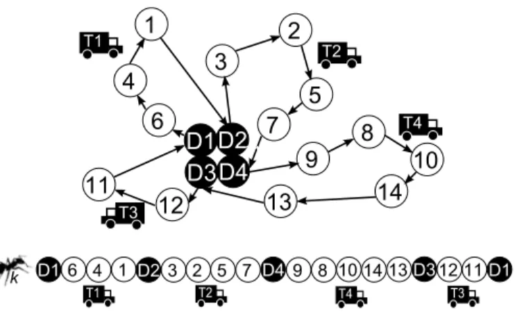
This scheme is easily extendable to the multi-vehicles case as follows. A virtual depot Dk
is created for each vehicle k. They are considered as new possible “clients” to visit, without demand and with a large time window. All the copies have the same coordinates. When the ant leaves a depot Dk, it corresponds to the beginning of a route for vehicle k, which
becomes the current vehicle. When the ant arrives in a depot Dk, it corresponds to the end
of the route of the current vehicle. If a depot Dk is not visited, then the associated vehicle k
is not used. A solution, denoted ψ, can be represented as a sorted list of clients and depots Dk to visit.
4 1 3 D1 D2 D3 D4 6 5 7 2 9 8 10 14 13 11 12 D1 6 4 1 D2 3 2 5 7 D4 9 8 10 14 13D312 11D1 T4 T1 T3 T1 T2 T4 T3 T1 T2 k
Figure 1: Structure of a route for one ant
When vehicle k leaves Dk, the corresponding vehicle properties are associated to the ant
and the clock is reset to the beginning of the planning horizon. While ψ is constructed successively one vehicle at a time, the time sequence is not strictly increasing. Each segment of the path between two copies Dk corresponds to one parallel time sequence. Time and
capacity usages are then computed as usual. If client j belongs to Ni,we get:
sj = max (si+ oi+ tij, aj) rj = ri− qj
where ri is initialized at the vehicle capacity C.
5
The ACS algorithm for the DVRPTWSD with
re-sponsiveness
We give first the outline of the algorithm and leave the details of the adaptations with respect to the standard ACS for the next subsections. We also provide a basic example at the end of the section to illustrate how all the characteristics are handled.
5.1
From the standard VRPTW to the DVRPTWSD with
re-sponsiveness
The algorithm for the problem at hand, limited first to the static context, is depicted in Algorithm 1. The general scheme of the ACS presented in the previous section is preserved. Until a time limit is reached (line 3), one ant at a time leaves the colony (line 4) to sequentially construct a tentative path ψ. A move from one location to the next one may be considered while there exists at least one client who can still be visited within the time window by a non-empty and compatible truck (loop starting line 10). Otherwise, the ant stops its attempt and the post-treatments start (line 13). Each move from the current location to the next one implies two steps. First, the next location is determined (lines 11) by calling the function SelectNextLocation (see Algorithm 2). Second, the move is executed from i to j (line 12) by calling the function MoveTo (see Algorithm 3). Next, if the final ant path does not go through all the clients, a procedure attempts to insert the missing customers (line 13). Some post-treatments occur (lines 14-18) each time one ant founds a path serving all the clients. It includes local search improvements, the update of the best solution and the pheromone
1 (R∗, ψ∗) ← Greedy heuristic ; // Initialization
2 τ0 ← 1
nR∗; τij ← τ0 ∀i, j ∈ N ; 3 while ¬ Time limit do
4 foreach Ant do // Main loop: one ant looks for a solution 5 Draw vehicle k ∈ V at random ;
6 Read vehicle status;
7 ψ ← {Dk} ; // Path initialization
8 i ← D ; // First location
9 wi ← 1st time of availability for k;
10 while ∃ client j who can be reached within its TW by a compatible truck do 11 j ← SelectNextLocation(i);
12 i ← MoveTo(j);
13 if All clients are not served then ψ ← Insertion procedure(ψ);
14 if All clients are served then // A solution ψ exists→ post-treatments 15 Update ψ to bring all the vehicles back to D;
16 Local search to eventually improve the current solution ψ;
17 if (Rψ < R∗) OR ((Rψ == R∗) AND (Tψ < T∗)) then (R∗, ψ∗) ← (Rψ, ψ); 18 foreach arc (i, j) ∈ ψ do τij = (1 − ρ)τij + ρτ0;// Update trail locally 19 foreach arc (i, j) ∈ ψ∗ do τij = (1 − ρ)τij+ ρ
R∗; // Update trail globally
Algorithm 1: Static ant colony algorithm
1 Function SelectNextLocation(i) 2 if (Ni == {D}) then j ← D;
3 else
4 foreach j ∈ Ni\ {D} do ηij ← 1
max(wi+tij,aj)+ok(j)j −aj
;
5 With probability d0, j ← D ; // Depot strategy 6 else With probability q0, j ← arg max
lτilηβil; // Exploitation 7 else Select j ∈ Ni\ {D} with probability
τijηijβ
P
l∈Niτilηβil ; // Exploration
8 Return j;
Algorithm 2: SelectNextLocation()
evaporation. Finally (line 19), when a group of ants has completed the search, the trail is globally updated based on the best current solution. In the dynamic context, the same algorithm is called repeatedly with a proper initialization of the inputs.
SelectNextLocation selects the next visit using the ant colony mechanisms: trail intensity, closeness, exploration and exploitation. A vehicle is only allowed to move to a feasible neighbor ∈ Ni. A client belongs to Ni if it has not yet been (fully) served, if the remaining
vehicle capacity is large enough to serve it and if the vehicle can be served before the end of the time window. This last constraint may be relaxed when considering soft time windows. We remove from this set the list of incompatible clients for the vehicle visiting i. MoveTo performs the move. The path ψ, the client status and the vehicle status are updated. The procedure differs when the next location is the depot (lines 2-8), or a client (lines 9-19).
1 Function MoveTo(j)
2 if (j == D) then // Either return to depot
3 rk← Ck;
4 New time of availability for k ← wi+ tiD+ ok D; 5 With probability ζ, restart with the same vehicle k; 6 else Draw vehicle k ∈ V at random;
7 ψ ← ψ + {Dk};
8 wD ← 1st time of availability for k;
9 else // ...or serve a client
10 ψ ← ψ + {j};
11 if (qj > rk) then // If this is a split delivery
12 wj ← wi+ tij + ok(j)
j with qj in ok(j) replaced by rk; 13 qj ← qj− rk for this ant;
14 aj ← wj for this ant;
15 rk← 0;
16 else // ... or not a split delivery
17 wj ← wi+ tij + ok(j)
j ;
18 rk← rk− qj;
19 j is marked as fully served; 20 Return j;
Algorithm 3: MoveTo()
5.2
Responsiveness criterion
We are concerned by situations where responsiveness is more critical than the distance traveled. The global objective, as defined in the problem description section, is to minimize the responsivenessPjsj+ o
k(j)
j − aj. In the ACS, the optimization of the objective function
is achieved through the closeness measure that we redefine as: ηij =
1 Rij
= 1
sj+ ok(j)j − aj
where Rij is the marginal responsiveness attached to the move from client i to client j.
A drawback to this measure is that the standard mechanism for determining the next move can no longer be used as such. In the previous mechanism, the closeness measure is used without differentiating between the depot and the clients. In our context, however, the depot and the clients have different structures for the time windows. For the depot, the window includes the entire planning horizon. Therefore, the depot is always eligible and the related closeness measure strictly increases with time. The more time goes into the construction of the path, the more the algorithm would suggest to bring the vehicle back to the depot. We can easily solve this issue by removing all the depots from the neighborhoods Ni and by
adapting the displacement strategy. Two cases occur. When there are no more clients in Ni,
the only feasible next move is going to the depot (line 11). Otherwise, we may allow, with a probability of d0 (line 14), the vehicle to go back early to the depot, or, with a probability
d0 is a parameter and could be left at zero to send the vehicles back to the depot only when
truly required. This is the typical strategy in practice in many cases. We suggest here to allow anticipated returns for two reasons. The first is in the context of a multi-trip strategy. We may hope that a vehicle fully replenished during intermediate periods (when the demand would be less intense) could be able to serve successively more clients later (during periods with more intense demand). Second, anticipated returns may allow construction of more balanced routes. Indeed, within the responsiveness framework, each vehicle is considered successively for constructing routes. It increases the probability that longer routes, in terms of number of clients, would be affected to the first selected vehicles. The sequence of vehicles is drawn at random and no vehicle is actually disadvantaged, but the process could still end with unbalanced routes. Note, however, that the local search described later, based on cross exchanges, naturally corrects this phenomenon. The anticipated return strategy remains an option in an attempt to improve the process at the level of the ACS. On the other hand, requiring the vehicles to come back in advance to the depot may prevent the construction of unbalanced routes. This question is solved by applying this strategy only to a subset of ants and by defining a dynamic value of d0. Any static value for d0 could be defined by the
user depending on the problem at hand. We propose a more dynamic strategy. Based on the first multi-trip motivation, sending back a vehicle is senseless if its remaining capacity is large. We first associate d0 with the percentage of emptiness ((Ck− rk)/Ck). Sending back
a vehicle every two moves on average when it is at half capacity would remain excessive. We next associate d0 with the average number of moves a vehicle would perform before being
empty. With q denoting the average demand, the typical number of moves would be Ck/q.
This leads to our proposal: d0 = q(CCk−r2 k) k .
In connection with the responsiveness criterion, there is another major difference between our approach and the traditional one: the size of the fleet. We consider fleets of vehicles belonging to the operator. The size of such a fleet cannot vary dynamically with respect to the demand and reducing the number of vehicles operating simultaneously does not have a strong impact on the cost structure. We therefore don’t try to minimize the number of vehicles in use. By contrast, an optimal solution in the context of the responsiveness criterion would naturally put as many vehicles to work as possible . Initializing the algorithm with a realistic fleet size limit is therefore compulsory. This contrasts with the results obtained when the criterion is based on the distance and where using fewer vehicles could be a way of reducing the distances. Note also that the responsiveness objective is not always contradictory to the minimization of the distances. Short distances imply short travel times, and short travel times facilitate an arrival at the beginning of the time windows. This becomes even more significant when responsiveness includes the travel time; for example when the beginning of a time window corresponds to the demand notification in the dynamic case. The shortest route is, however, not guaranteed to be the optimal one. We check this assertion in the experiments.
5.3
Heterogeneous fleet
The main adaptation of the algorithm for the heterogeneous fleet, beside the definition of the closeness measure as a function of ok
j, is done at the level of the neighborhoods Ni
constructions. Before considering the addition of client j to Ni, we must ensure that client
j doesn’t belong to the list of incompatible clients for the vehicle leaving i. The specific operating time ok
on the departure times from each client j, a specific vehicle k may or may not be able to reach another client in time. For all three of these components, we need to know which vehicle is arriving at client j. Since one depot Dk was created as a starting point for each
vehicle k, it suffices to check which was the last parking visited by the ant.
When dealing with a heterogeneous fleet, another concern is the allocation process of the depots during the construction of the route. Until now, the depots were considered equivalent and it made no difference for an ant to start or to come back to one or another depot. This is no longer the case with a heterogeneous fleet. Considering all the depots successively in one sequence would always favor the same vehicles which is not optimal. Therefore, to allow full exploration, each vehicle is drawn at random at the beginning of a new tour (lines 5 and 21).
5.4
Multi-trip
Lots of companies operate continuously seven days a week. The operating day can be long or even unbounded. Therefore, the vehicles are allowed to come back to the depot for replenishment (lines 17-23). The depot is managed as a client to be served and the service corresponds to the replenishment. A specific operating time for replenishment, still with constant and variable parts, is associated to each vehicle (ok
D line 19). After this operation,
the vehicle is available again and can start a new trip to a new client. While in the basic algorithm the initial departure time from the depot is set to the beginning of the planning horizon, this can no longer be the case when the same vehicle is allowed to start new trips. After each replenishment and before a new eventual departure, the initial time associated to the vehicle must be reset to the time of completion of the last replenishment (lines 19 and 23).
Note that the next vehicle to be considered by default for departure after a replenishment in Algorithm 1 is drawn at random. Another strategy would be to restart with the vehicle which was just replenished. This would lead to a more intensive use of the same vehicles and, in some extreme cases, possibly to a reduction in the number of vehicles operating. In our context, the fleet belongs to the operator and its size cannot be instantaneously adapted. Minimizing the number of vehicles on the road does not lead to significant benefits since it has no impact on the fixed costs. Moreover, it could be a counterproductive strategy when the fleet and the demands are highly heterogeneous. We have therefore integrated a mechanism in the ACS algorithm to permit the intensification of the use of the same vehicles. When selecting the next Dk as a starting point, the last vehicle used in the current solution
is selected with a probability ζ; otherwise, another vehicle is drawn at random. By setting ζ to zero, we obtain the original algorithm.
5.5
Split delivery
Split delivery also requires some adaptations of the ACS algorithm (lines 26-30). First, a client j is no longer rejected from the neighborhood Niwhen the only constraint unsatisfied is
a remaining capacity inferior to the demand. However, to speed up the optimization process, we still reject vehicles that would not be able to deliver a quantity larger than a minimal threshold set by the operator. Due to the initialization and travel times, such solutions would later be discarded and the work of the ant lost. Next, the client is not marked visited (to be opposed to line 34)and its demand is reduced by the quantity already delivered (line
28). Moreover, if we don’t want to allow several simultaneous deliveries, the beginning of the time window for client j is set to the time of the end of the last partial delivery (line 29). To the process, client j appears as a “new” classical client yet to be served. This strategy is valid since only one ant is used to construct all the routes for each vehicle and the construction process is sequential. Finally the first vehicle has no other alternative (due to line 30) than to next go back to the depot, where, thanks to the multi-trip strategy, it can reset its capacity and hit the road again to serve any unserved client.
5.6
Dynamic stochastic environment
We now extend the previous algorithm to the dynamic stochastic context. In our ap-proach, new events and new information can be integrated into the process over time. As in Gendreau et al. (1999), our strategy is to restart the optimizer each time new information is available. Another strategy, as in Montemanni et al. (2005), would be to slice the days into sub-periods and to optimize again only at these moments. The former has the advan-tage of taking into account any change immediately. Since responsiveness is the main goal, delaying the use of information would be counterproductive. On the other hand, if the pro-cess requires a long computation time to get a good (local) optimum, optimizing too often with a strict limit on computation time would risk reducing the quality of the intermediate plannings. Fortunately, our heuristic is fast and, at least for our experiments, good results can be achieved very quickly on modern computers.
Implementing dynamism into the ACS requires several adaptations. First, for each opti-mization, vehicles can be anywhere and not only at the depot. Second, we must keep track of the remaining capacity of each vehicle for each new start. The vehicle capacity and loca-tion quesloca-tions are simply solved by a correct initializaloca-tion of the ACS parameters (line 6). Instead of the full nominal capacity, each vehicle starts with the real current capacity. In-stead of starting from the depots (lines 7-8,22), we set the departure locations at the current observed location for each vehicle. If a new piece of information requesting an optimization arrives while a vehicle is still serving a client or moving to another location, then this vehicle is marked available only after completing this current operation. It is therefore important to associate with each vehicle the time wi at which it becomes available again (with i being
the vehicle location after completing the current operation). This time can be later than the time at which the new optimization occurs. We also have to determine the location i and the remaining capacity rk of each vehicle after the completion of the operation in progress.
In order to facilitate these reoptimizations and to handle stochasticity, we designed a PhP interface. Before each new optimization, the code computes the theoretical situation according to the previous planning i.e. the locations of the vehicles, the remaining capacities and the demands still to satisfy. The dispatcher only has to adjust the data, if necessary, based on new information he has received since the last optimization.
5.7
A small illustration
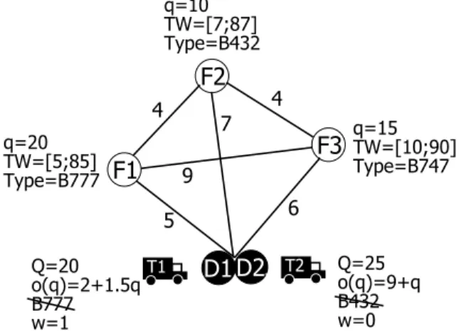
To illustrate the previous mechanisms, imagine that two trucks are available to serve three flights as depicted in Figure 2. The distances, corresponding to the travel times, are indicated on each arc. The quantities q, time windows and types of the aircrafts are indicated beside each node. The fleet is heterogeneous. Truck 1 has a lower capacity (Q = 20) than Truck 2 (Q = 25) but has a faster service time when the quantity to deliver is less than 14 units.
Truck 1 (resp. Truck 2) is not convenient and cannot be used for Boeing 777 aircrafts (resp. Boeing 432). This implies that Flight 1 (resp. Flight 2) can only be served by Truck 2 (resp. Truck 1). Moreover, we assume in this example that Truck 1 is initially still operating somewhere and cannot be used before one unit of time has passed. Split deliveries are allowed, but any delivery must be larger than five units when the demand is larger.
Figure 2: A small illustration
When constructing a path, an ant could consider up to 60 distinct sequences of moves before reaching a feasible solution or a first infeasibility. If the trucks are allowed to return to the depot for replenishment only when there are no more flights in their neighborhood, then only two paths are feasible. These two solutions are represented in the top right corner of Figure 2 (Ants 1 and 2). Four other solutions are feasible when the trucks may come back to the depot at any time (d0 > 0 - Ants 3 up to 6). Solution 1 is detailed in Table 1.
In solution 1, a first truck, Truck 1, is initially selected at random to take into account the heterogeneity of the fleet. Truck 1 leaves the depot (D1) to first serve Flight 2 and then
Flight 3. Responsiveness after serving Flight 2 is equal to 18; the difference between the completion time w (25) and the start of the time window (7). When arriving at Flight 3’s location, its remaining capacity is 10 units while the demand is larger (15 units). A split delivery occurs for 10 units. Truck 1 completes this first part of the delivery at time 46. The second part of the delivery cannot start before the completion of the first part. Flight 3 will appear in the sequel as a new client with a time window starting at time 46 and with a demand of 5 units of fuel. Truck 1 must then go back, empty, to the depot. Truck 2 is then considered. It leaves at time 0 (w = 0) to reach Flight 1’s location. After serving Flight 1, it goes to Flight 3 to serve the five remaining units of fuel. It arrives at Flight 3’s location at time 43 but has to wait until time 46 because Truck 1 is, according to the time line, still serving Flight 3 (new time window). All the services (s) started after the beginning a of each time window and were completed before the end b. The responsiveness R amounts to 97 units of time and the traveled distance T to 37 units.
Ant 2 illustrates a multi-trip solution. The ant first starts with Truck 2 and visits Flight 1. The remaining capacity (five units of fuel) is not large enough to serve any other flights and the truck must come back to the depot for replenishment. Truck 1 is then operated to fully serve Flight 2 and partially serve Flight 3. To complete Flight 3’s delivery, Truck 2 restarts a new trip after replenishment. As for Ant 1, the first part of Flight 3’s delivery ends at time 46. Due to its first tour and the replenishment, Truck 2 may only arrive at time
Path sequence D1 2 3 [D1] D2 1 3 [D2]
Time window: start (a) 0 7 10 0 0 5 10→46 0
Time window: end (b) 96 87 90 96 96 85 90 96
Travel time (t) 0 7 4 6 0 5 9 6
Service starts at (s) 0 8 29 52 0 5 43→46 66
Service duration (o) 0 17 17 32 0 29 14 34
Service completed at (w) 1 25 46 84 0 34 60 100
Quantity delivered (q) 0 10 10 -20 0 20 5 -25
Truck remaining capacity (r) 20 10 0 20 25 5 0 25
Responsiveness (R) 0 18 18 18 18 47 97 97
Distance (T ) 0 7 11 17 17 22 31 37
Table 1: Feasible path for ant 1
74 for completing Flight 3’s delivery, significantly increasing the final responsiveness (125). Ants number three through six consider anticipated returns to the depot. These solutions appear less natural and are indeed not beneficial, at least for this example.
All other sequences of visits are eluded by the ant optimization process. Indeed, the neighborhood definitions prevent such paths. Three cases are illustrated in Figure 2 by the ants 7, 8 and 9. Ant 7 attempts to start with Truck 1. Visiting Flight 1 after leaving D1 is
rejected since this aircraft, a B777, is incompatible with Truck 1. Ant 8 illustrates a violation of a time window. It is not possible to visit Flight 3 after replenishing Truck 1 since Truck 1 would not be able to complete the operation before time 99.5, i.e. after the end of the time window (90). Ant 9 illustrates a problem of insufficient capacity. No flight is in the neighborhood of Flight 1 for Truck 2 since its remaining capacity is five units of fuel at this time, which is less than the minimal allowed quantity for a split delivery and less than what is required by the other flights (10 and 15).
Another important insight from this illustration is that optimizing responsiveness or distance does not lead to equivalent solutions. The path for the most responsive solution (Ant 1) is longer (37 units) than the shortest solution (36 units). Conversely, the responsiveness for the shortest solution (116.5 units of time) is far less attractive than the most responsive solution (97). Note also that the shortest path would not have been encountered without allowing trucks to return in advance to the depot (d0 > 0).
5.8
Back to the distance criterion
Considering responsiveness instead of distance is of critical importance in many applications. Thus, the focus of this work is on responsiveness. Minimizing the length of routes obviously remains an attractive question in many other contexts. It is also scientifically interesting to compare routes obtained with these two different objectives. While Algorithm 1 was developed with a responsiveness criterion in mind, it can easily be adapted to use the distance criterion instead,; going back to the procedures defined in Section 4 for the objective and the closeness measure. The implementation of all the other constraints remains valid. Primarily, the closeness measure must be replaced based on the distance (line 13), each Ni\ {D} by Ni
(lines 11 and 16) and the probabilistic return to the depot (line 14) suppressed. Finally, R has to be replaced by T . In the results section, the two versions are executed on benchmarks found in the literature in order to compare the responsive routes with the shortest ones.
6
Initialization and improvements
We discuss here how to initialize the ACS and, as a side effect, how to get some benchmarks for the responsiveness criterion. We also present some methods to improve the solutions provided by the ants.
6.1
Initial solutions
A first feasible solution is required to initialize τ0. A classical approach is to use a nearest
neighbor heuristic. A sequence of visits is constructed one at a time for each vehicle. In the sequence, the nearest client of i in the feasible neighborhood Ni is selected. Ni is defined
as in the ant colony algorithm and therefore takes into account all the dimensions of the problem. The nearest client is defined as the one for which the client responsiveness is the smallest. If two clients have the same responsiveness, the tie is broken by minimizing the distance. When we replace the objective of responsiveness by a traditional criterion, the nearest client remains the closest one.
This first heuristic does not adequately suit a responsiveness criterion. In practice, dis-patchers in airports use another basic approach, simply serveing the clients by order of arrival. The main loop is therefore no longer on the vehicles, but on the clients. Within the pool of vehicles available and compatible at the start of a client time window, we select the one which is idle for the longest time. This heuristic, named F IF O for First In First Out, may serve as a tool to identify an initial feasible solution and to compute τ0, but it is
also a benchmark with which to compare our results to standard practice. Note that this benchmark assumes, in the dynamic case, that the vehicle starts to move to reach a client i only after ai since a dispatcher typically waits until the start of the time window for all the
latest information. It therefore implies that the client will always have to wait, at least for the travel time. In a deterministic case and to better take into account the heterogeneity of the fleet, a variation of this heuristic allows the vehicle to start to the client as soon as the vehicle is available, and the preferred vehicle is the one which incurs the smallest responsive-ness for the client. This variant, denoted F IF O2, is used to compute the initial solution. If we want to replace the responsiveness criterion with a more traditional minimization of the distance, the same heuristic remains valid. The preferred vehicle for a client simply becomes the nearest one. One additional approach is sometimes considered in practice. The dispatch-ers initially plan the journey deterministically as in the F IF O approach. A list of clients is then associated with each driver, but here he has to follow this list even if new events occur. Along the course of the operating day and with the arrival of new information, each driver adapts the plan using the F IF O heuristic but only considering his vehicle and his list of clients. This second strategy is clearly less efficient than the F IF O one but corresponds to another reality of operations. Since it will always provide a larger value for the objective function, we do not use it in the sequel.
6.2
Local searches
When an ant has completed its search (line 36 of Algorithm 1), the solution might be in-complete. As suggested in Gambardella et al. (1999), the algorithm attempts to reconstruct a local solution by inserting the remaining clients in the path . For each client, the best insertion in the current tours is kept if such an insertion exists. Gambardella et al. (1999)
considers each client by decreasing demand. In our responsiveness and richer context, we ob-tained better results by selecting the clients in a random order. Finally, to preserve the spirit of the ant colony and to avoid spending too much time here, the insertion procedure is only started when the ant provides a significantly long solution (for our numerical experiments, at least 75% of the clients must be visited by the ant before initiating insertions).
Even when the ant, with or without insertions, provides a local feasible optimum, it is well known that performance can generally be improved by combining the ACS with local search procedures (line 39). As suggested again in Gambardella et al. (1999), we developed a local search basic heuristic based on CROSS exchanges (Taillard et al. (1997)). Such an operation consists of permuting two sub-chains of clients belonging to two different vehicles. One of the sub-chains could be empty, leading to a more traditional insertion. Both sub-chains could also end at the depot leading to a 2-opt edges exchange. In our na¨ıve algorithm, we only apply a few CROSS exchanges such that it improves the objective each time. Each vehicle is tested in a random order in conjunction with a second one. Since CROSS exchanges imply two vehicles, we also tested a local search limited to one vehicle at a time. Each client is successively moved to another position in the same tour. The best move, if any, is kept.
6.3
Pheromone conservation
As a final improvement, we have included in the algorithm the pheromone conservation procedure developed by Montemanni et al. (2005). The idea is to pass valuable information from one optimization to the next one in the dynamic context. Indeed, the problems under consideration from one optimization to the next one generally share lots of characteristics since the most recent one is an adaptation of the previous one. The optimal paths of the first problem are therefore good candidates for the next problem. Since the attractiveness of a path is stored in the pheromone matrix, the idea is to stop initializing this matrix by only using the results of a heuristic, but instead by mixing it with past information. For each pair of clients which appear both in the old and in the new problem, the corresponding pheromone matrix entry is initialized to the following value:
τij = (1 − γ)τijold+ γτ0
where τold
ij is the pheromone intensity associated to the path between client i and client j
at the end of the previous optimization, τ0 is the default pheromone value computed by the
initialization heuristic and γ is a parameter controlling the level of conservation. We slightly adapt this scheme. Since the clients are typically not exactly the same from one optimization to the next, the orders of magnitude of τold
ij and τ0 could be different. We therefore use this
formula instead: τij = (1 − γ)τijold τ0 τold 0 + γτ0 where τold
0 is the initial value of the pheromones in the previous optimization. τ0old is used in
the local updating scheme and can be seen as the basic or neutral level of pheromones. τ0
τold 0
can then be interpreted as a scaling factor to the new context.
7
Results
The approach is tested on real and simulated instances. The code is written in Java. All results were obtained on a standard laptop operating Windows 8. An online web interface
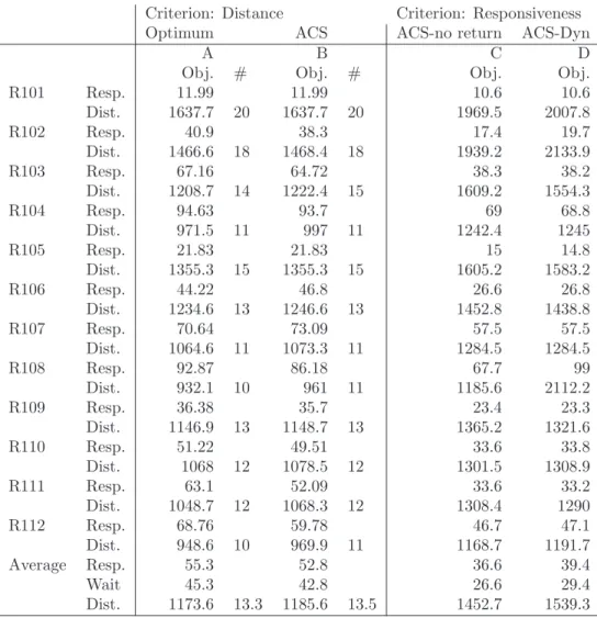
written in PhP is also available. We further analyze the performance of the ACS using two sets of benchmarks. To our knowledge, no benchmark exists that allows us to simultaneously consider all the characteristics of the types of problems we are faced with here, especially in regard to the responsiveness criterion. We therefore start from a set of well-known VRP benchmarks used in the literature and initially designed for the distance criterion. Each of these two sets of benchmarks exhibits some of the characteristics of our problem. In the first case, we analyze the impact of a dynamic strategy when new events/demands are added into the schedule during operations. In the second case, we work in a static context on VRPs with time windows using one set of Solomon’s benchmarks. In both cases, we endeavor to replicate results found in the literature when the criterion is distance, and we extend them to responsiveness.
7.1
Airport problem
We first test the ACS on a real case provided by our partner: Liege Airport (LGG). LGG is the 8th biggest cargo airport in Europe and received the World’s Best Cargo Airport Airport of the Year Award for the quality of its management in Singapore in 2013. The goal is to develop a decision system to optimize the journey of the refueling trucks. We consider a representative night of operations. 30 aircrafts, of seven different models, are expected during the next three hours and must be refueled within one hour of landing. During this tight schedule, there are many time window overlaps and possibilities to plan the truck journeys. Up to five trucks were used during this night but some of them are not able to serve certain types of aircraft. The service operating time depends on the aircraft and on the selected truck and takes ten minutes on average. The parking spaces are mainly along a straight road, which induces lots of symmetries in the problem. Split deliveries may occur if the truck can serve at least 1500L. For confidentiality reasons, the flight names are replaced by fake names and we set the start of the operations at time zero. Data is available on our website.
The ACS algorithm is initialized with standard values for VRP. Exploration (q), closeness weight (β) and pheromone update (ρ) parameters are respectively set to 0.9, 1 and 0.1. The longer the optimization process runs, the higher the probability is to find the optimal or at least an improved solution. However, there is a limited amount of time available in practice to find a solution. It is especially limited in the dynamic context. We therefore limit the computation time in all the experiments. We test different reasonable limits as specified in the next tables. Ten ants start from the colony at each iteration.
Many simulations were conducted using this configuration and some variations. The most representative ones are displayed in Table 2 and Table 3. The selected parameters are given in the first five lines of each table, while the next lines are the corresponding results. Table 2 summaries the results for the responsiveness criterion in a deterministic context. Table 3 provides results when the criterion is distance. Table 3 also contains results for the responsiveness criterion in a dynamic case where new information is provided throughout the day and new optimizations occur. Responsiveness is the total time the 30 aircrafts must stay on the ground before refueling is completed. It includes the operating service time and the idle time, where the idle time is the time spent by the aircraft waiting for the arrival of a truck. We provide the average and maximal idle time per aircraft. We also provide the safety time as a measure, on average and as a minimum, of time left before the theoretical departure. This can be seen as a buffer that could absorb an unexpected event or as an
opportunity to reduce the time on the ground, therefore saving costs.
A B C D E F G H
Objective: Resp. Resp. Resp. Resp. Resp. Resp. Resp. Resp.
Algorithm: FIFO FIFO2 ACS ACS ACS ACS ACS ACS
Max CPU time : - - 1h 5’ 5’ 30” 30” 30”
Local searches: No No Yes No Yes Yes Yes Yes
Back to depot: - - Dynamic Dynamic Dynamic Dynamic None Dynamic
Truck intensity: 0 0 0 0 0 0 0 1
Responsiveness: 11h33 10h00 9h00 9h08 9h03 9h03 9h04 9h03
Distance (m): 35550 32253 26984 27252.8 27928.2 27928.2 25422.6 27129.3
Average idle time: 9.1’ 6.2’ 4.2’ 4.4’ 4.2’ 4.2’ 4.2’ 4.2’
Max idle time: 25.1’ 30.1’ 32.5’ 28.9’ 34’ 34’ 34’ 34’
Average safety time: 37.1’ 40’ 41.9’ 41.7’ 41.9’ 41.9’ 41.8’ 41.9’
Min safety time: 17.2’ 13.8’ 3.7’ 5.6’ 2.2’ 2.2’ 2.2’ 2.2’
Table 2: Airport case: responsiveness criterion in a deterministic context
Some general comments may be made regarding these simulations. First, thanks to the ACS, it is always possible to organize the trips so that each flight is served on time, so that the average idle time is low and so that the average safety time is high. This is already a significant outcome for the airports. This instance is complex. Many flights arrive in the same short interval of time and the total demand corresponds roughly to the total fleet capacity. In this context, multiple trips have a high cost and each truck should therefore be used at its maximum capacity during each tour. We observe that each of the five trucks are operated. We also observe that split deliveries never occur in the optimal solutions, which can be explained by the extra (constant) time required to operate more than one truck for a same client that makes this operation unattractive. Note, however, that one truck returns to the depot for replenishment before restarting for serving a late flight. Applying local searches always improves the quality of the solutions and speeds up the process (compare case E vs. case D). Allowing the trucks to come back to the depot at any time (d0 > 0 and a dynamic strategy based on the remaining vehicle capacity) has a slightly positive impact (compare case F vs. case G). Actually, there is no major difference in the quality of the solutions if the optimization process is allowed to run longer, but this simulation and the tests on the Solomon’s benchmarks later indicate that the process often converges faster. As mentioned previously in the illustration with a small example, it also important in order to cover all the domain. Finally, the impact of intensifying the use of a same truck is not clear. It has no significant impact for this instance when responsiveness is the main criterion (case F vs. case H), and it has a slightly negative impact when the criterion is distance (case K vs. case L).
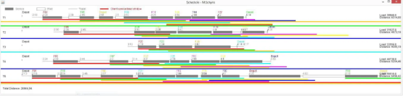
Table 2 provides more details with regard to the operational quality of the results in the deterministic context for the responsiveness criterion. Case F provides a solution with an objective value of only 9h03 in 30 seconds of CPU computation time. Very few new improved solutions are found when the allocated CPU time increases. A similar result is obtained in five minutes (case E). 9h00 is the best solution found (case C) but it requires one hour of computation time. This solution is depicted in Figure 3. This is a strong performance with respect to three benchmarks. First, imagine that the airport applies a traditional FIFO strategy (case A) as described in the previous section. The total responsiveness would
Figure 3: Optimal schedule (Case C)
amount for 11h33, meaning that the ACS approach is able to improve responsiveness by 22%. Second, if it was possible to apply the second strategy FIFO2, which is not realistic in a dynamic context, FIFO2 would perform better than the FIFO strategy but would still remain far less attractive at 10h00, than the ACS solution. It shows that a very basic heuristic can already provide an interesting solution with respect to the FIFO rule, at least when the objective is responsiveness optimization, but also that an Ant Colony can still make a significant difference. Finally, we can investigate whether 9h00 is the global optimum. Unfortunately we have no tool to prove this. We can still compute a lower bound. Assuming that the fastest operating truck is able to serve an aircraft immediately without generating idle time, then, based on the quantities to be delivered, it would require at least 6h30 of operations (i.e. responsiveness). This corresponds to an average difference of five minutes per aircraft in comparison with the best ACS solution. Note also that it is a very optimistic lower bound since we made two strong assumptions that can clearly not be satisfied in this context of intense demand.
Analyzing the performances of the ACS approach when the objective is to minimize the distance rather than optimizing the responsiveness is also enlightening. Cases I to L indicate that the ACS algorithm is able to find good solutions with respect to this other criterion. The best result with a distance of 17877m is obtained after one hour (case I). A very close result, 17968m, is already obtained after 30 seconds (case K). More interestingly, we can compare the solutions when we use distance instead of responsiveness as the criterion. These two different objectives lead to drastically different tours. Assuming that optimizing the responsiveness is of crucial importance for some companies, minimizing the distance in the hope that a shorter set of routes will imply a higher speed of service and a better responsiveness is erroneous. In our case, the shortest tour (case I) is associated with a responsiveness of 16h03, which is far inferior to the most responsive solution (case C: 9h00). Even the typical FIFO strategy (case A) does better with 11h33. We also observe a large variation of the responsiveness for solutions of approximately the same length, which in itself shows that responsiveness is not directly linked to distance. When (tight) time windows exist, two elements explain this difference. First, the time associated with a trip is no longer calculated as the distance divided by the speed since the vehicles have to wait if they arrive in advance by a client. Distance divided by speed is only a lower bound. Second, responsiveness time is also lower than the time for the fastest tour since responsiveness is measured with respect to the start of the client time window and not with respect to the time of departure from the previous client; i.e. a subset of this last interval. Conversely, when optimizing the distance is of crucial importance, optimizing the responsiveness is not an adequate strategy. It leads to solutions 50% longer for this instance (17876m vs. 27253m) or as high as two times longer
if we compare with the FIFO strategy (35550m). When responsiveness is the criterion in opposition to distance, we also observe that the aircrafts do not need to wait as long before being served, and that there is a vast buffer period before planned departure. Moreover, the average idle time per aircraft is reduced by a factor four when responsiveness is considered instead of distance. This is an important and attractive operational result.
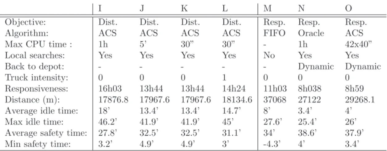
I J K L M N O
Objective: Dist. Dist. Dist. Dist. Resp. Resp. Resp.
Algorithm: ACS ACS ACS ACS FIFO Oracle ACS
Max CPU time : 1h 5’ 30” 30” - 1h 42x40”
Local searches: Yes Yes Yes Yes No Yes Yes
Back to depot: - - - Dynamic Dynamic
Truck intensity: 0 0 0 1 0 0 0
Responsiveness: 16h03 13h44 13h44 14h24 11h03 8h038 8h59
Distance (m): 17876.8 17967.6 17967.6 18134.6 37068 27122 29268.1
Average idle time: 18’ 13.4’ 13.4’ 14.7’ 8’ 3.4’ 4’
Max idle time: 46.2’ 41.9’ 41.9’ 45’ 27.6’ 25.4’ 26’
Average safety time: 27.8’ 32.5’ 32.5’ 31.1’ 34’ 38.6’ 37.9’
Min safety time: 3.2’ 4.9’ 4.9’ 3’ -4.3’ 4’ 3.4’
Table 3: Airport case: distance and dynamic contexts
The previous results only discuss the algorithm in a static context for which all the information is known precisely in advance. With cases M, N and O, we now discuss the performances of the approach in a stochastic environment. Throughout the operating day, new events occur. The landing time and the beginning of each time window are not known with certainty. To simulate this, we draw at random the beginning of each time windows ai. We use a Gaussian probability distribution centered on the previously used expectation
time and with a standard deviation corresponding to fifteen minutes. When the size of the time windows after shifting its beginning becomes greater than one hour or smaller than 30 minutes, the (expected) end of the time window is adjusted to maintain a standard one hour window for the operations. If the resulting ai is smaller than the previously expected time,
the dispatcher is informed ten minutes before ai. Otherwise, he gets the new information
at the initially expected time of arrival. The true quantities to deliver are communicated precisely at the beginning of each (new) time window. They are computed thanks to a normal distribution centered on the expected quantities and with a standard deviation corresponding to 10% of the expected quantities. Finally, the service time is sometimes faster and sometimes slower than expected by a value distributed once more according to a normal distribution N(0,3). This information is made available during the service. All in all, in this simulation scheme, new information appears at 42 different moments during the operating day of the 30 flights.
Case O provides the final results obtained when a new optimization is performed each time a new piece of information appears, leading to 42 runs. The shortest delay between the arrival of two new pieces of information was one minute. Due to this level of granularity, each new optimization was allowed to run for only a fraction of one minute, more precisely 40 seconds. This ensures real time operations. Thanks to our approach, it was always possible to adapt the planning to serve all the flights in time. We also observe that the results are very good. To determine this, first note that the average idle time is very low and the safety time very large, which is attractive to the airports. The minimum safety time of only 3.4