Calibrating Activity-Based Models with External OD Information: Overview Of Different Possibilities

1 2 3 4 5 6 7 8 9 10

CALIBRATING ACTIVITY-BASED MODELS

11

WITH EXTERNAL OD INFORMATION:

12

AN OVERVIEW OF DIFFERENT POSSIBILITIES

13 14 15

Mario Cools, Elke Moons, Geert Wets* 16

17

Transportation Research Institute 18 Hasselt University 19 Wetenschapspark 5, bus 6 20 BE-3590 Diepenbeek 21 Belgium 22 Fax.:+32(0)11 26 91 99 23 Tel.:+32(0)11 26 91{31, 26, 58} 24

Email: {mario.cools, elke.moons, geert.wets}@uhasselt.be 25 26 27 28 * Corresponding author 29 30 31 Number of words = 5670 32 Number of Figures = 3 33 Number of Tables = 7 34

Words counted: 5670+ 10*250 = 7670 words 35

36

Revised paper submitted: November 15, 2009 37

38 39 40 41

ABSTRACT

1 2

Many practitioners question the advantages of activity-based models over conventional four-step 3

models in terms of replication of traffic counts. Therefore, in this paper, a framework is 4

highlighted that actively links travel demand models in general, and activity-based models in 5

particular, with traffic counts. Two approaches are presented that calibrate activity-based models 6

with traffic counts, namely an indirect and a direct approach. The indirect approach tries to 7

incorporate findings, based on the analysis of traffic counts, into the model components of the 8

activity-based models. The direct approach calibrates the parameters of the travel demand model 9

in such a way that the model replicates the observed traffic counts (quasi-)perfectly. A practical 10

example is provided to illustrate the direct approach. The study area for this practical example is 11

Hasselt, a Belgian city of about 70,000 residents, and its surrounding municipalities. The 12

practical examples revealed that there is not a single roadway to success in calibrating activity-13

based models, but that different options exist in fine-tuning the activity-based model. 14

Notwithstanding, it is important to recognize some open issues and avenues for further research. 15

First, it is not always appropriate to assume that traffic counts are completely correct. Setting up 16

some belief-structure might increase the responsiveness of the activity-based model. In addition, 17

the OD-matrix calibration that optimizes the correspondence between estimated and observed 18

screen-line counts could negatively impact the correspondence to other measures such as vehicle 19

miles traveled. To conclude, formulation of a multi-objective calibration method is a key 20

challenge for further research. 21

1 BACKGROUND

1 2

Due to an increased environmental awareness, current travel demand models pursue higher 3

levels of behavioral realism. Four periods can be distinguished in this evolution of travel demand 4

modeling approaches. The first period, the late 1950’s, is a period typified by a steep increase in 5

car use. During this period, trip-based models were developed to make long term projections of 6

travel demand in order to assess major investments in road infrastructure. These first generation 7

models assumed that travel is the result from four consecutive steps, namely trip generation, trip 8

distribution, mode choice and route choice (1). From the mid 1970’s until the 1990’s, the focus 9

shifted towards the travel needs of a single person. The original four-step models were replaced 10

by theories about utility maximizing behavior and individual choice behavior. Discrete choice 11

models such as multinomial logit models and more advanced statistical techniques formed the 12

core of so-called tour-based systems (2). From the mid 1990’s and early 2000’s activity-based 13

travel demand models became a rising modeling paradigm. The basic premise of these third 14

generation models is the fact that travel behavior is a derivative from the activities that an 15

individual performs (1). Current dynamic activity-based models, such as Aurora and Feathers 16

(3), taking into account different forms of learning could be seen as a fourth generation of travel 17

demand models. 18

Although modern activity-based travel demand models have clear theoretical advantages 19

over conventional four-step models – the most important ones are the fact that all basic travel 20

decisions can be applied in a disaggregate fashion, the explicit linkages between the travel 21

decisions of members of a single household, the consistent choices for a single person across all 22

travel decisions and the disaggregate way of handling the time-of-day of travel decisions – 23

conventional models still dominate the travel demand modeling paradigm (4,5). Davidson et al. 24

(6) highlighted several reasons that explain the acceptance of and resistance to more 25

sophisticated model frameworks. They can be broadly categorized as the degree of resistance to 26

new modeling technology and the size of encouragement forces. The reasons include the size of 27

the public agency, the size of the jurisdiction, the level of institutional history and the level of 28

state support for travel demand forecasting. Davidson et al. (6) also stressed that in order to 29

reinforce the transition from conventional models towards activity-based models, it is imperative 30

that the objective theoretical advantages of activity-based models are better explained to 31

practitioners and communicated more actively. 32

This paper focuses on a concern that stems from misunderstanding and mistrust by 33

practitioners. Although researchers have acknowledged the advantages of an exhibited 34

behavioral realism to policy analysis, many practitioners question the advantages of activity-35

based models over conventional four-step models in terms of replication of traffic counts, as it is 36

in many respects easier to adjust a conventional travel demand model to fit base level traffic 37

counts exactly than an activity-based micro-simulation model (6). In this regard, it is important 38

to stress the distinction between static model accuracy in terms of the replication of the base-39

year observed data, and the responsive properties of the model that are related to the quality of 40

the travel forecasts for future and changed conditions, as these two model properties do not 41

necessarily coincide. Therefore, in this paper, different techniques are highlighted that actively 42

link activity-based models in particular, and travel demand models in general, with traffic counts 43

in order to achieve the desired responsive properties – the model being sensitive to demographic 44

changes and policy measures – of the travel demand models as well as the replication of traffic 45

counts. Note that proper calibration is a crucial step in simulation models as findings based on 46

inappropriately calibrated models could be misleading and even erroneous (7). An overview of 1

new calibration and validation standards, as well as best practice examples for travel demand 2

modeling, is provided by Schiffer and Rossi (8). Bare in mind that the calibration of an activity-3

based model is not unlike calibrating a conventional four-step model (5). A thorough example of 4

the calibration of a conventional four-step model with traffic counts is provided by Cascetta and 5

Russo (9). For an excellent example concerning the calibration of an activity-based travel 6

demand model (i.e. the Sacramento activity-based travel demand model) the reader is referred to 7

Bowman et al. (10). 8

The remainder of the text is organized as follows. Section 2 provides an outline of the 9

suggested techniques that are implemented in a practical example, which are thoroughly 10

discussed in Section 3. Finally, some general conclusions and avenues for further research are 11

indicated. 12

13

2 LINKAGES BETWEEN ACTIVITY-BASED MODELS AND TRAFFIC COUNTS

14 15

There are two possible approaches to link activity-based models in particular, and travel demand 16

models in general, with traffic counts, namely an indirect and a direct approach. The first 17

approach tries to incorporate findings, based on the analysis of traffic counts, into the model 18

components of the activity-based models. The second approach calibrates the model parameters 19

of the activity-based model in such way that the model replicates the observed traffic counts 20

(quasi-)perfectly (less than 5% error on average). The following subsections will elaborate and 21

further clarify the two methods of linking activity-based models with traffic counts. 22

23

2.1 Indirect Linkage

24 25

The ‘indirect linkage’-approach tries to identify events that affect travel behavior and resulting 26

traffic patterns. Analysis of traffic counts for instance can be used to identify effects of holidays 27

and weather events (11). These traffic swaying events can then be used to alter the impedance 28

functions used in route choice modules. When events such as holidays and weather conditions 29

are identified, their impact on travel behavior can even be further elucidated by analyzing 30

activity diary data. Utility functions that express the propensity of performing certain activities – 31

note that basically the utility functions of all elements of the activity-pattern generation can be 32

modified in this way – can then explicitly incorporate explanatory variables to account for the 33

events that were analyzed. In this regard, activity-diary collection tools that integrate 34

geographical information logging, such as the PARROTS-tool (12) provide the required data to 35

perform detailed analysis, for instance on route choice. It can be expected that the explicit 36

incorporation of events that account for the variability in revealed traffic patterns and their 37

underlying reasons, will result in both an improved responsiveness of the activity-based model 38

and a better replication of traffic counts. 39

40

2.2 Direct Linkage

41 42

The ‘direct linkage’-approach tries to fine-tune the model parameters of the activity-based (AB) 43

model in such a way that the model-based traffic counts correspond maximally to the observed 44

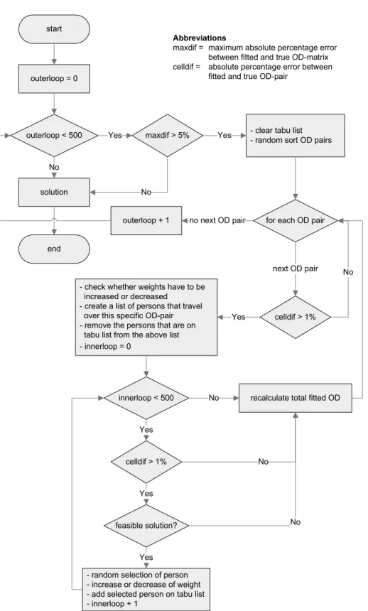
ones on the network. Calibration opportunities exist at four levels (Figure 1): the data level, the 45

model level, the OD-matrix level and the assignment level. 46

1 2

FIGURE 1 Four levels of calibration opportunities.

3 4

Two approaches can be followed when considering calibration at the data level: a ‘crude’ 5

approach, where data (personal/household information, zonal information) is altered in order to 6

achieve a better correspondence to the benchmark measures, and a ‘fine’ approach where agents 7

(individuals or households) are weighted. The first approach immediately raises questions 8

concerning the validity and the credibility: adjusting fields or adding or deleting records 9

undermines the validity of the model and should be avoided. The latter approach attributes 10

weights to the different agents. For the practical example discussed in Section 3, the weights are 11

chosen to be natural numbers (including zero) such that these weights correspond to exact 12

counterparts in the real population. Fractional weights like 0.8 or 1.2 would also have been 13

feasible, but the interpretation of these weights would be a probability of this agent to have an 14

exact counterpart in the real population (0.8 would correspond to a change of 80% of having an 15

exact counterpart in the real population, and 1.2 would be interpreted as 80% chance of having 16

one counterpart in the real population, 20% of having two counterparts in the real population). 17

The use of weights can be justified by the fact that there exist groups of individuals with similar 18

travel behavior that can be captured in representative activity patterns (RAPs). By using these 19

RAPs, the complete activity-generation can be performed in a hands-on manner (13). McNally 20

(14) and Wang (15) have even further advocated the use of RAP’s by showing that RAP’s are 21

relatively stable over conventional planning horizons (up to 10 years). Weighting agents thus 22

seems to be a worthwhile path to follow. Notwithstanding, the weighting procedure can become 23

computationally very intensive as the number of possible weights increases with the number of 24

simulated agents. 25

A second calibration possibility arises at the model level. The activity schedule 26

generation could be altered in such a way that the obtained OD-matrix optimally reproduces the 27

observed traffic counts. One solution to achieve this optimal state is an ‘updating’-process which 28

alters the scheduling rules that are derived from the available travel survey data. In addition, 29

zone-specific rules can be introduced: for instance increasing the probability of certain 30

destination choices, or increasing the probability of performing a certain activity. In that way, 31

the production and attraction of these zones can be fine-tuned. When different forecasting 32

scenarios are desired, it is necessary to keep the updated rules that were defined by the updating-33

process in the baseline year. In that manner the AB-model is constructed in a consistent way. 34

Hence, linking activity-based models with traffic counts by making behavioral adjustments 35

(altering rules) might prove to be a valid way of overcoming practitioners’ mistrust. 36

The matrix level is the third level at which calibration opportunities arise. The OD-37

matrix is obtained by the simultaneous activity schedule execution of all agents. This OD-matrix 38

can then be benchmarked in function of the screen-line counts. Different techniques exist to 39

estimate OD-matrices from traffic counts. In practice, most models assume or require that a 40

target OD-matrix is available. This target OD-matrix (the OD-matrix resulting from the activity-41

based model) is a crucial part of prior information. In statistical approaches, the target OD-42

matrix is typically assumed to stem from a sample survey and is regarded as an observation of 43

the “true” OD-matrix. The observed set of traffic count data may also be assumed to be an 44

observation of the “true” traffic count data, and therefore (small) deviations between estimated 45

counts and observed counts may be accepted. Thus, the purpose of the calibration process is to 1

find an OD-matrix which produces “small” differences between the estimated link flows and the 2

observed flows. Three modeling philosophies are postulated in the transportation literature (16): 3

traffic modeling based approaches, statistical inference approaches and gradient based solution 4

techniques. 5

The traffic assignment module is the last level where calibration is possible. Obviously 6

the way of attributing origin-destination flows to the network plays a crucial role in how well the 7

model-based traffic counts correspond to the benchmark measures. Ortúzar and Willumsen (17) 8

classify traffic assignment methods according to their treatment of congestion (inclusion of 9

capacity restraints) and their treatment of differences in objectives and perceptions by agents 10

(inclusion of stochastic effects). 11

12

3 PRACTICAL EXAMPLE

13 14

In this section, a numerical example is provided to further illuminate the ‘direct linkage’-15

approach. The study area for this numerical example is Hasselt, a Belgian city of about 70,000 16

residents, and its surrounding municipalities. Activity-travel information derived from census 17

data, from the Flemish travel survey and from the origin-destination (OD) matrix assigned in the 18

multimodal travel demand model Flanders, is combined to generate a simulated “true” 19

population and its corresponding travel behavior. The data from this true population is assumed 20

to be unbiased and precise. For generating the “true” representative activity patterns (RAPs) at 21

population level, people are supposed to perform activities in a predefined order: first, people 22

perform a work or school activity, then they go shopping, afterwards they perform a leisure trip, 23

and finally, they perform other type of activities. In addition to this predefined order, it is 24

presumed that people perform a specific type of activity at most once (the exact chances to 25

perform a specific activity are given in the upper part of Table 1). Furthermore, it is assumed 26

that residents return home after their last activity. 27

To focus on the general ideas behind the different calibration techniques presented, and 28

to reduce model complexity, route choice modeling (traffic assignment) and mode choice 29

modeling were not taken into account. Thus, the practical example focuses on the first three 30

levels of calibration. Assuming perfect knowledge about these aspects procures the property that 31

the quality of the output of the (activity-based) travel demand model is completely related to the 32

aggregated OD-matrix resulting from the individual activity patterns. In addition, owing to the 33

perfect knowledge of these aspects, traffic counts on the different roads form an identity match 34

to the destination flows. Note that the assumption of perfect knowledge about origin-35

destination relationships nowadays become a more viable option. When privacy issues are 36

explicitly addressed, data from a mobile phone network can be used to derive origin-destination 37

patterns (18). Results from Caceres et al. (19) and González et al. (20) indicate that extracting 38

OD-information from mobile phone records has great potential and is much more cost-efficient 39

that those generated with traditional techniques. 40

As complete information about all activity-patterns seldom is available, the starting point 41

for the calibration exercises is a 2.5% stratified random sample of the “true” population 42

(municipality is taken as the stratification variable). The lower part of Table 1 provides more 43

information about the 2.5% sample: the number of residents in each municipality, as well as the 44

municipality specific propensities to perform different activities, are displayed. 45

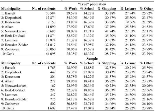
TABLE 1 Number of Residents and Propensities of Activity Participation

1 2

“True” population

Municipality No. of residents % Work % School % Shopping % Leisure % Other

1: Hasselt 70 584 29.59% 14.22% 33.28% 27.94% 25.92% 2: Diepenbeek 17 874 34.30% 30.49% 30.47% 25.30% 23.47% 3: Kortessem 8 153 33.83% 16.39% 33.88% 19.66% 21.59% 4: Alken 11 090 27.92% 17.60% 37.76% 25.35% 24.82% 5: Nieuwerkerken 6 685 28.02% 17.71% 41.74% 22.03% 22.11% 6: Herk-De-Stad 11 874 32.52% 21.32% 35.20% 21.10% 23.61% 7: Lummen 13 874 31.38% 16.38% 37.03% 21.19% 21.77% 8: Heusden-Zolder 31 017 24.54% 17.95% 32.19% 24.18% 23.63% 9: Zonhoven 20 060 30.06% 17.57% 31.42% 24.32% 24.79% 10: Genk 64 095 25.35% 18.32% 28.77% 25.85% 23.79% Sample

Municipality No. of residents % Work % School % Shopping % Leisure % Other

1: Hasselt 1 765 28.90% 13.88% 32.52% 30.71% 25.89% 2: Diepenbeek 447 35.35% 27.07% 30.43% 23.27% 23.94% 3: Kortessem 204 35.78% 14.22% 31.37% 25.98% 21.57% 4: Alken 277 29.96% 18.41% 36.82% 24.55% 23.83% 5: Nieuwerkerken 167 23.95% 20.36% 40.72% 23.35% 20.96% 6: Herk-De-Stad 297 32.32% 18.86% 36.03% 21.55% 22.56% 7: Lummen 347 28.82% 20.46% 35.73% 24.50% 20.46% 8: Heusden-Zolder 775 24.13% 16.52% 33.29% 25.81% 21.16% 9: Zonhoven 502 30.88% 22.71% 34.06% 26.89% 26.10% 10: Genk 1 602 27.47% 17.04% 28.34% 25.22% 23.78% 3

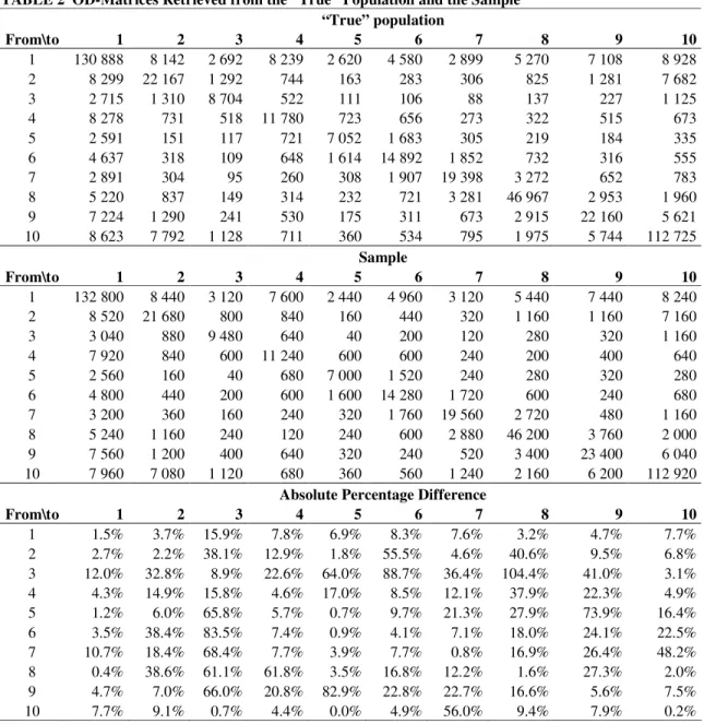
Table 2 presents the OD-matrix obtained from aggregating the individual activity persons 4

from all people in the population (upper part of the Table 2) and the sample (lower part of the 5

Table 2). The OD-information from the sample is scaled up to the population level for 6

comparison purposes. A side-note has to be made concerning the “true” population origin- 7

destination matrix. When the origin-destination flows of this matrix are compared to flows really 8

observed in practice, the population OD-matrix overestimates the flows observed in practice. 9

This is due to the fact that all residents from the municipalities in this practical example are 10

assumed to perform their activities within the entire study area. 11

The absolute percentage difference (APE) between the true population and the sample is 12

displayed in the lower part of Table 2. Many of these APEs are larger than 5% indicating that 13

some extra calibration is needed to improve the correspondence with the “true” observed values. 14

The absolute percentage is defined as: 15

(

)

where T_ij represents the number of trips from municipality i to municipality j, pop indicates that 17

the flow corresponds to the population, and sa that the flow corresponds to the sample. A 18

possible infinity value could be one, indicating that you are of the target by 100%. Such an 1

infinity value has to be defined, as many calculations are infeasible when values are divided by 2

zero (and thus mathematically are equal to infinity). Since the “true” population OD-matrix 3

contains no zero cells, no infinity value had to be defined in the practical example. 4

5

TABLE 2 OD-Matrices Retrieved from the “True” Population and the Sample

6 “True” population From\to 1 2 3 4 5 6 7 8 9 10 1 130 888 8 142 2 692 8 239 2 620 4 580 2 899 5 270 7 108 8 928 2 8 299 22 167 1 292 744 163 283 306 825 1 281 7 682 3 2 715 1 310 8 704 522 111 106 88 137 227 1 125 4 8 278 731 518 11 780 723 656 273 322 515 673 5 2 591 151 117 721 7 052 1 683 305 219 184 335 6 4 637 318 109 648 1 614 14 892 1 852 732 316 555 7 2 891 304 95 260 308 1 907 19 398 3 272 652 783 8 5 220 837 149 314 232 721 3 281 46 967 2 953 1 960 9 7 224 1 290 241 530 175 311 673 2 915 22 160 5 621 10 8 623 7 792 1 128 711 360 534 795 1 975 5 744 112 725 Sample From\to 1 2 3 4 5 6 7 8 9 10 1 132 800 8 440 3 120 7 600 2 440 4 960 3 120 5 440 7 440 8 240 2 8 520 21 680 800 840 160 440 320 1 160 1 160 7 160 3 3 040 880 9 480 640 40 200 120 280 320 1 160 4 7 920 840 600 11 240 600 600 240 200 400 640 5 2 560 160 40 680 7 000 1 520 240 280 320 280 6 4 800 440 200 600 1 600 14 280 1 720 600 240 680 7 3 200 360 160 240 320 1 760 19 560 2 720 480 1 160 8 5 240 1 160 240 120 240 600 2 880 46 200 3 760 2 000 9 7 560 1 200 400 640 320 240 520 3 400 23 400 6 040 10 7 960 7 080 1 120 680 360 560 1 240 2 160 6 200 112 920

Absolute Percentage Difference

From\to 1 2 3 4 5 6 7 8 9 10 1 1.5% 3.7% 15.9% 7.8% 6.9% 8.3% 7.6% 3.2% 4.7% 7.7% 2 2.7% 2.2% 38.1% 12.9% 1.8% 55.5% 4.6% 40.6% 9.5% 6.8% 3 12.0% 32.8% 8.9% 22.6% 64.0% 88.7% 36.4% 104.4% 41.0% 3.1% 4 4.3% 14.9% 15.8% 4.6% 17.0% 8.5% 12.1% 37.9% 22.3% 4.9% 5 1.2% 6.0% 65.8% 5.7% 0.7% 9.7% 21.3% 27.9% 73.9% 16.4% 6 3.5% 38.4% 83.5% 7.4% 0.9% 4.1% 7.1% 18.0% 24.1% 22.5% 7 10.7% 18.4% 68.4% 7.7% 3.9% 7.7% 0.8% 16.9% 26.4% 48.2% 8 0.4% 38.6% 61.1% 61.8% 3.5% 16.8% 12.2% 1.6% 27.3% 2.0% 9 4.7% 7.0% 66.0% 20.8% 82.9% 22.8% 22.7% 16.6% 5.6% 7.5% 10 7.7% 9.1% 0.7% 4.4% 0.0% 4.9% 56.0% 9.4% 7.9% 0.2% 7

3.1 Calibration at the Data Level

8 9

The goal of weighting agents is to procure the highest possible resemblance between the 10

observed traffic counts on the network and the predicted traffic counts by the activity-based 11

model. In the non-calibrated model all agents are equally weighted (weights equal to the inverse 12

of the sample size). By iteratively altering the weights, an optimal correspondence can be found 13

using meta-heuristics (a meta-heuristic is a general algorithmic framework that can be used to 1

guide heuristic methods to search for feasible solutions to different optimization problems). Two 2

different approaches can be distinguished when agents have to be weighted. The first approach 3

weights the agents before their activity pattern is generated. Since agents are duplicated before 4

the activity patterns are generated, the activity patterns of the replicated agents - created by the 5

weights – can differ from the ones of the “true” agents. Thus, the convergence of the iterative 6

process of weighting persons and calculating the activity patterns of the “agents” and their 7

replicates is not necessarily guaranteed. The second approach solves this convergence problem 8

by weighting the activity patterns instead of the agents themselves. Take for example a resident 9

in Hasselt, who only performs a work activity in Diepenbeek. From Table 2 one can see that if 10

this persons weight would be decreased, both the estimated OD-flows from Hasselt to 11

Diepenbeek and Diepenbeek to Hasselt would be reduced, and thus be closer to the “true” OD-12

flows for the population. 13

To illustrate the calibration of OD-matrices at the data levels, the second approach, the 14

weighting of activity patterns, is followed. The RAPs of the residents in the sample are weighted 15

using the algorithm displayed in Figure 2. Note that the algorithm that is implemented includes 16

an element originating from tabu search meta-heuristics, namely the concept of a tabu list. A 17

tabu list is a short-term memory where, in this case, the persons whose weights have been 18

altered, are stored (21). The tabu list ensures that these weights are not altered multiple times 19

within the same iteration, thus preventing situations like for instance the repetitive increasing 20

and decreasing of the weight of a specific person. Two versions of the algorithm were 21

implemented. The first one changed the weights by adding or subtracting one. The second one 22

altered the weights by increasing or reducing the weights by a random number between one and 23

ten, reducing the risk of converging towards the same saddle point (i.e. the same (sub)-24

optimum). A safeguard was included, procuring non-negative weights. 25

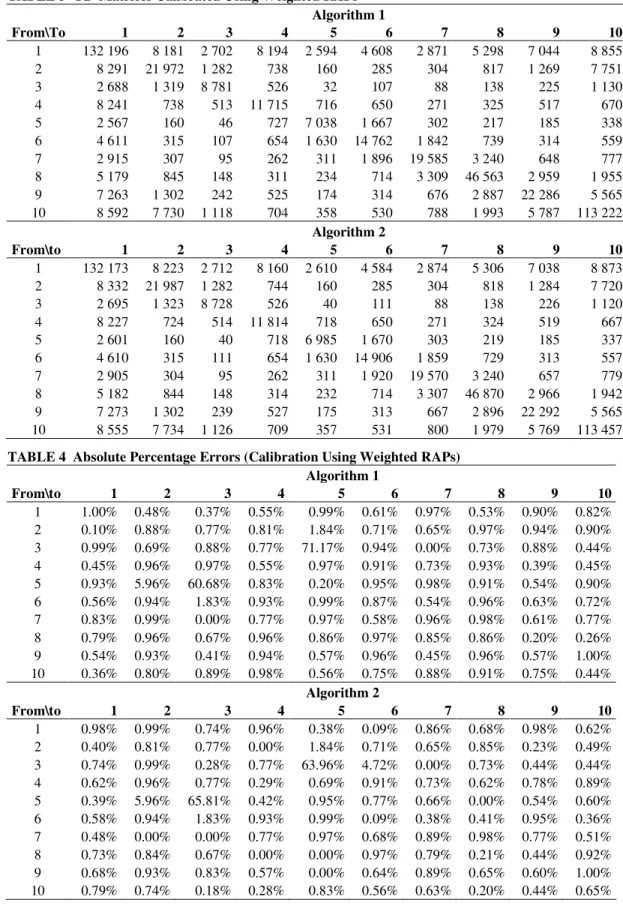
The estimated OD-matrices are provided in Table 3. The mean absolute percentage error 26

(MAPE) of the estimated matrix using the first algorithm equals 2.12%, whereas the second 27

matrix has a MAPE of 2.02%. From Table 4 one could notice that for two cells in both matrices 28

the APE is higher than 0.5. This is due to the fact that the very few people are traveling between 29

these two locations (Kortessem and Nieuwerkerken), and in line with this, that the persons in the 30

sample travelling between these locations, also travel between other uncommon OD-pairs 31

(Kortessem – Herk-De-Stad and Kortessem – Lummen). This underlines the importance of 32

including a stop criterion in the algorithms to avoid an endless computation. 33

outerloop = 0

solution

- random selection of person - increase or decrease of weight - add selected person on tabu list - innerloop + 1

outerloop < 500

for each OD pair

innerloop < 500 No

maxdif > 5% Yes

- check whether weights have to be increased or decreased

- create a list of persons that travel over this specific OD-pair - remove the persons that are on

tabu list from the above list - innerloop = 0

recalculate total fitted OD - clear tabu list

- random sort OD pairs

No Yes no next OD pair celldif > 1% feasible solution? celldif > 1% next OD pair _No Yes Yes Yes Yes No No No start outerloop + 1 end Abbreviations

maxdif = maximum absolute percentage error between fitted and true OD-matrix celldif = absolute percentage error between

fitted and true OD-pair

1

FIGURE 2 Calibration algorithm to weight representative activity patterns.

2 3 4

TABLE 3 OD-Matrices Calibrated Using Weighted RAPs 1 Algorithm 1 From\To 1 2 3 4 5 6 7 8 9 10 1 132 196 8 181 2 702 8 194 2 594 4 608 2 871 5 298 7 044 8 855 2 8 291 21 972 1 282 738 160 285 304 817 1 269 7 751 3 2 688 1 319 8 781 526 32 107 88 138 225 1 130 4 8 241 738 513 11 715 716 650 271 325 517 670 5 2 567 160 46 727 7 038 1 667 302 217 185 338 6 4 611 315 107 654 1 630 14 762 1 842 739 314 559 7 2 915 307 95 262 311 1 896 19 585 3 240 648 777 8 5 179 845 148 311 234 714 3 309 46 563 2 959 1 955 9 7 263 1 302 242 525 174 314 676 2 887 22 286 5 565 10 8 592 7 730 1 118 704 358 530 788 1 993 5 787 113 222 Algorithm 2 From\to 1 2 3 4 5 6 7 8 9 10 1 132 173 8 223 2 712 8 160 2 610 4 584 2 874 5 306 7 038 8 873 2 8 332 21 987 1 282 744 160 285 304 818 1 284 7 720 3 2 695 1 323 8 728 526 40 111 88 138 226 1 120 4 8 227 724 514 11 814 718 650 271 324 519 667 5 2 601 160 40 718 6 985 1 670 303 219 185 337 6 4 610 315 111 654 1 630 14 906 1 859 729 313 557 7 2 905 304 95 262 311 1 920 19 570 3 240 657 779 8 5 182 844 148 314 232 714 3 307 46 870 2 966 1 942 9 7 273 1 302 239 527 175 313 667 2 896 22 292 5 565 10 8 555 7 734 1 126 709 357 531 800 1 979 5 769 113 457 2

TABLE 4 Absolute Percentage Errors (Calibration Using Weighted RAPs)

3 Algorithm 1 From\to 1 2 3 4 5 6 7 8 9 10 1 1.00% 0.48% 0.37% 0.55% 0.99% 0.61% 0.97% 0.53% 0.90% 0.82% 2 0.10% 0.88% 0.77% 0.81% 1.84% 0.71% 0.65% 0.97% 0.94% 0.90% 3 0.99% 0.69% 0.88% 0.77% 71.17% 0.94% 0.00% 0.73% 0.88% 0.44% 4 0.45% 0.96% 0.97% 0.55% 0.97% 0.91% 0.73% 0.93% 0.39% 0.45% 5 0.93% 5.96% 60.68% 0.83% 0.20% 0.95% 0.98% 0.91% 0.54% 0.90% 6 0.56% 0.94% 1.83% 0.93% 0.99% 0.87% 0.54% 0.96% 0.63% 0.72% 7 0.83% 0.99% 0.00% 0.77% 0.97% 0.58% 0.96% 0.98% 0.61% 0.77% 8 0.79% 0.96% 0.67% 0.96% 0.86% 0.97% 0.85% 0.86% 0.20% 0.26% 9 0.54% 0.93% 0.41% 0.94% 0.57% 0.96% 0.45% 0.96% 0.57% 1.00% 10 0.36% 0.80% 0.89% 0.98% 0.56% 0.75% 0.88% 0.91% 0.75% 0.44% Algorithm 2 From\to 1 2 3 4 5 6 7 8 9 10 1 0.98% 0.99% 0.74% 0.96% 0.38% 0.09% 0.86% 0.68% 0.98% 0.62% 2 0.40% 0.81% 0.77% 0.00% 1.84% 0.71% 0.65% 0.85% 0.23% 0.49% 3 0.74% 0.99% 0.28% 0.77% 63.96% 4.72% 0.00% 0.73% 0.44% 0.44% 4 0.62% 0.96% 0.77% 0.29% 0.69% 0.91% 0.73% 0.62% 0.78% 0.89% 5 0.39% 5.96% 65.81% 0.42% 0.95% 0.77% 0.66% 0.00% 0.54% 0.60% 6 0.58% 0.94% 1.83% 0.93% 0.99% 0.09% 0.38% 0.41% 0.95% 0.36% 7 0.48% 0.00% 0.00% 0.77% 0.97% 0.68% 0.89% 0.98% 0.77% 0.51% 8 0.73% 0.84% 0.67% 0.00% 0.00% 0.97% 0.79% 0.21% 0.44% 0.92% 9 0.68% 0.93% 0.83% 0.57% 0.00% 0.64% 0.89% 0.65% 0.60% 1.00% 10 0.79% 0.74% 0.18% 0.28% 0.83% 0.56% 0.63% 0.20% 0.44% 0.65%

3.2 Calibration at the Model Level

1 2

The basic model that will be calibrated, first predicts activity chains for all persons (the 3

proportions of the different activity chains have been fixed to the population proportions), and 4

then predicts the locations where the different activities will be performed. Note that the 5

proportions of the different activity chains have been fixed to the population proportions. This 6

ensures that discrepancies between the “true population” matrix, and the calibrated OD-7

matrix are only due to differences in destination choices (location probabilities). Thus, at the 8

model-level, the activity schedule generation could be altered by iteratively updating the 9

probabilities of certain destination choices (related to their respective activity purposes). The 10

adjustment of the model parameters is straightforward in this case as only one dimension is 11

considered at a time (i.e. the location probabilities). After all, the other parameters (such as the 12

chances of performing certain activities) are kept constant. For real activity-based models in 13

practice, a chain of interlinked choices with feedbacks are modeled, and thus multiple 14

parameters have to be changed simultaneously. This would seriously augment the complexity of 15

the model, but the basic framework elucidated in this paper, still could be used. 16

The updating process will attain a quasi-perfect match when the updated sample 17

probabilities of the destination choices are equal to the unknown population probabilities. 18

Nonetheless, a full search of the solution space (investigating all possible combinations of 19

location probabilities for the different activities) is not a feasible option, as the number of 20

possible combinations approaches infinity. The number of possible combinations can be 21

computed as follows: 22

(

)

(

)

1/ 1-precision of location probability × ,

23

which for the practical example discussed in this paper (applying a precision of 1%) would yield 24

a total number of possible combinations of 10500 (approximating infinity). Therefore, an 25

algorithm that explores the solution space for a ‘good’ solution instead of the optimal solution 26

should be implemented. 27

In order to calibrate the activity-based travel demand model, and to ensure convergence 28

of optimization algorithms, it is essential that the variability caused by the activity-generation 29

process is reduced as much as possible. Stability of the activity-generation can be ensured by 30

taking averages over multiple (activity-generation) runs, so that differences between the 31

estimated OD-matrix and the true population OD-matrix are not the result of random variations, 32

but of the altered location probabilities. However, guaranteeing the stability of the activity 33

generation diminishes the performances, as computation times are significantly increased. The 34

algorithm that is used is shown in Figure 3. 35

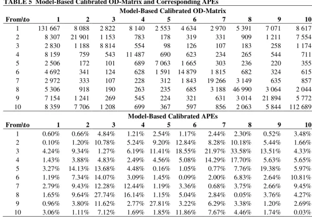
Table 5 presents the OD-matrix and corresponding APEs for the model-based calibration 36

results. From these results, one could see that here is a decrease in the mean absolute percentage 37

error from 20,27% in the up-scaled sample matrix to 6,29% in the model-calibrated OD-38

matrix (after 100 iterations). Nevertheless, as multiple activity-generations are required in each 39

step of the algorithm, model-based calibration is the most computer-intensive calibration option, 40

favoring other calibration techniques. 41

solution loop < 100 No best maxdif > 5% Yes No start end Abbreviations

maxdif = maximum absolute percentage error between fitted and true OD-matrix mape = mean absolute percentage error

between fitted and true OD-matrix locprob = activity location probabilities - loop = 0

- calculate locprob sample - calculate maxdif sample - calculate mape sample - best mape = mape sample - best maxdif = maxdif sample - best OD-matrix = OD-matrix sample - best locprob = locprob sample random sort activity types best mape > 2% Yes No

- random select OD-pair - load best locprob - increase locprob of

selected OD-pair - equalize sum locprob to 1 - actvity regeneration - calculate mape - calculate maxdif Yes for each activity type

next activity type

mape < best mape yes

no next activity type - best mape = mape

- best maxdif = maxdif - best locprob = locprob - best OD-matrix =

OD-matrix

- load best locprob - decrease locprob of

selected OD-pair with opposite of increase - locprob minimum 1 - equalize sum locprob to 1 - activity regeneration - calculate mape - calculate maxdif

no

mape < best mape yes no

loop + 1

1

FIGURE 3 Calibration algorithm to adjust activity location probabilities.

TABLE 5 Model-Based Calibrated OD-Matrix and Corresponding APEs

1

Model-Based Calibrated OD-Matrix

From\to 1 2 3 4 5 6 7 8 9 10 1 131 667 8 088 2 822 8 140 2 553 4 634 2 970 5 391 7 071 8 617 2 8 307 21 901 1 153 783 178 319 331 909 1 211 7 554 3 2 830 1 188 8 814 554 98 126 107 183 258 1 174 4 8 159 759 543 11 487 690 623 234 265 544 711 5 2 506 172 101 689 7 063 1 665 303 236 220 355 6 4 692 341 124 628 1 591 14 879 1 815 682 324 615 7 2 972 333 107 228 312 1 843 19 266 3 149 635 857 8 5 306 918 190 263 235 685 3 188 46 990 3 064 2 044 9 7 154 1 241 269 545 224 321 631 3 014 21 894 5 772 10 8 359 7 706 1 208 699 367 597 856 2 063 5 844 112 689

Model-Based Calibrated APEs

From\to 1 2 3 4 5 6 7 8 9 10 1 0.60% 0.66% 4.84% 1.21% 2.54% 1.17% 2.44% 2.30% 0.52% 3.48% 2 0.10% 1.20% 10.78% 5.24% 9.20% 12.84% 8.28% 10.18% 5.44% 1.66% 3 4.24% 9.34% 1.27% 6.19% 11.41% 18.55% 21.97% 33.58% 13.51% 4.33% 4 1.43% 3.88% 4.83% 2.49% 4.56% 5.08% 14.29% 17.70% 5.63% 5.65% 5 3.27% 14.13% 13.68% 4.48% 0.16% 1.05% 0.77% 7.76% 19.38% 5.97% 6 1.19% 7.34% 14.07% 3.09% 1.45% 0.09% 2.00% 6.83% 2.64% 10.81% 7 2.79% 9.43% 12.28% 12.44% 1.19% 3.36% 0.68% 3.75% 2.66% 9.45% 8 1.65% 9.64% 27.74% 16.14% 1.15% 5.04% 2.84% 0.05% 3.76% 4.27% 9 0.96% 3.80% 11.62% 2.77% 27.81% 3.22% 6.29% 3.38% 1.20% 2.69% 10 3.06% 1.11% 7.12% 1.69% 1.85% 11.86% 7.67% 4.46% 1.74% 0.03% 2 3

3.3 Calibration at the Matrix Level

4 5

The third level of calibration tackled in this study is the matrix level. Recall that perfect 6

knowledge about route choice and mode choice is assumed, and that an identity match is 7

presumed between traffic counts and origin-destination flows. Therefore the calibration at the 8

matrix level, like the two previous calibration levels discussed, is illustrated using OD-pair 9

information. The reader is referred to Abrahamsson (16) for a thorough literature review 10

concerning the calibration of OD-matrices using traffic counts. Three situations are explored in 11

order to calibrate the survey OD-matrix. 12

13

3.3.1 Perfect Knowledge about Inter-Zonal Traffic 14

15

In the first situation, it is assumed that “perfect” knowledge is available about all inter-zonal 16

traffic flows, but that information about intra-zonal traffic is only available at survey level. Let 17

i ij j

P =

∑

i

A =

∑

number of trips arriving in municipality j (attraction), and T_ij the number of trips from zone i to 19

zone j. Then the intra-zonal traffic flows (T_{ij i j,}= ) could be approached by the following formula:

20

(

)

(

)

(

)

, 1

est pop est pop

ij i j i i j j

T λ P P∗ λ A A∗

= = − + − − ,

where λ∈

[ ]

in a municipality, compared to the number of trips arriving in a municipality, where est indicates 2

that the quantity is derived from the estimated (survey) OD-matrix, and pop indicates that the 3

quantity is derived from the population “true” OD-matrix. The asterisk underlines that the fact 4

that the intra-zonal traffic flows are not included in the population row ( ,

, pop pop i ij j j i P∗ T ≠ =

∑

=

∑

accurately than attraction (17), in this practical example three times more confidence is placed in 7

the estimation of productions than in the estimation of attractions. Thus, the intra-zonal origin-8

destination flows are calculated as follows: 9

(

)

(

)

, 0.75 0.25

est pop est pop

ij i j i i j j

T = = P −P∗ + A −A∗ .

10

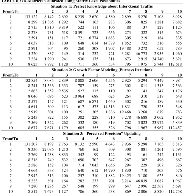
The resulting OD-matrix is given in the upper part of Table 6. Note that when it is assumed that 11

the activity-travel pattern of people begin and end in the home location (like it is the case for the 12

practical applications described in this paper), the number of trips originating from a 13

municipality equals the number of trips arriving in that municipality. In this case the choice of λ

14

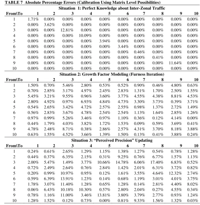
is irrelevant. From Table 7 it is clear that only the intra-zonal trips are altered (APEs for inter-15

zonal trips equal zero). 16

17

3.3.2 Growth Factor Modeling (Furness Iteration) 18

19

The second situation considers the case in which two OD-matrices (one on population level and 20

one derived from the sample) are available. Information from these OD-matrices can be 21

combined using growth factor modeling. One option is to take the cell information from the 22

population (e.g. retrieved from GPS tracks) and the trip totals (column and row totals of the OD-23

matrix) from the survey. A second option is the reverse, namely taking the cell information from 24

the survey, and the trip totals from the population. To illustrate the technique, the first option is 25

implemented. This option is the more realistic one, as in practice precise OD-pair information 26

can be derived using cell phone information at fairly low costs, while surveys capture well the 27

total travel demand. The doubly constrained growth factor model is estimated using Furness 28

iterations. Formally, the number of trips from municipality i to j (T_ij) is calculated as follows: 29

ij ij i j T =t ×a ×b , 30

where t_ij is the number of trips (in the population OD-matrix), and where a_i and b_j are 31

balancing factors. These balancing factors are a set of correction coefficients which are 32

appropriately applied to the cell entries in each row or column. The iterative procedure starts 33

with setting all b_j equal to one. In the second step, the a_i are solved for b_j to satisfy the trip 34

production constraint (row totals of the cell entries of the population OD matrix have to equal 35

the productions derived from the survey). Subsequently, in the third step, the b_j are solved for 36

the a_i, calculated in the previous step, to satisfy the trip attraction constraint (column totals of 37

the cell entries of the population OD matrix have to equal the attractions derived from the 38

survey). Then, the OD matrix is updated. This consecutive calculation of a_i and b_j is repeated 39

until convergence is achieved (both the production and attraction constraints are satisfied). The 40

procedure yields the matrix presented in the middle of Table 6, the corresponding APEs in Table 1

7. 2 3

TABLE 6 OD-Matrices Calibrated Using Matrix Level Possibilities

4

Situation 1: Perfect Knowledge about Inter-Zonal Traffic

From\To 1 2 3 4 5 6 7 8 9 10 1 133 122 8 142 2 692 8 239 2 620 4 580 2 899 5 270 7 108 8 928 2 8 299 21 365 1 292 744 163 283 306 825 1 281 7 682 3 2 715 1 310 9 819 522 111 106 88 137 227 1 125 4 8 278 731 518 10 591 723 656 273 322 515 673 5 2 591 151 117 721 6 774 1 683 305 219 184 335 6 4 637 318 109 648 1 614 14 379 1 852 732 316 555 7 2 891 304 95 260 308 1 907 19 488 3 272 652 783 8 5 220 837 149 314 232 721 3 281 46 773 2 953 1 960 9 7 224 1 290 241 530 175 311 673 2 915 24 740 5 621 10 8 623 7 792 1 128 711 360 534 795 1 975 5 744 112 618

Situation 2: Growth Factor Modeling (Furness Iteration)

From\To 1 2 3 4 5 6 7 8 9 10 1 132 854 8 085 2 839 8 008 2 606 4 556 2 925 5 294 7 449 8 984 2 8 241 21 536 1 333 707 159 275 302 811 1 313 7 563 3 2 863 1 352 9 535 527 115 110 92 143 247 1 176 4 8 046 695 523 10 964 688 625 264 310 517 648 5 2 577 147 121 687 6 871 1 640 302 216 189 330 6 4 611 309 113 617 1 573 14 513 1 831 720 325 548 7 2 919 301 100 251 305 1 886 19 468 3 268 679 783 8 5 243 822 155 302 228 710 3 278 46 688 3 062 1 952 9 7 569 1 322 262 532 180 319 702 3 023 23 972 5 839 10 8 677 7 671 1 179 685 355 526 796 1 967 5 967 112 457

Situation 3: “Perceived Precision” Updating

From\To 1 2 3 4 5 6 7 8 9 10 1 131 207 8 192 2 763 8 132 2 590 4 643 2 936 5 298 7 163 8 813 2 8 336 22 086 1 210 760 162 309 308 881 1 261 7 595 3 2 769 1 238 8 833 542 99 122 93 161 242 1 131 4 8 218 749 532 11 690 702 647 267 302 496 667 5 2 586 152 104 714 7 043 1 656 294 229 207 326 6 4 664 338 124 640 1 612 14 790 1 830 710 303 576 7 2 942 313 106 257 310 1 882 19 425 3 180 623 846 8 5 223 891 164 282 233 701 3 214 46 839 3 087 1 967 9 7 280 1 275 267 548 199 299 647 2 996 22 367 5 691 10 8 512 7 673 1 127 706 360 538 869 2 006 5 820 112 758 5

TABLE 7 Absolute Percentage Errors (Calibration Using Matrix Level Possibilities)

1

Situation 1: Perfect Knowledge about Inter-Zonal Traffic

From\To 1 2 3 4 5 6 7 8 9 10 1 1.71% 0.00% 0.00% 0.00% 0.00% 0.00% 0.00% 0.00% 0.00% 0.00% 2 0.00% 3.62% 0.00% 0.00% 0.00% 0.00% 0.00% 0.00% 0.00% 0.00% 3 0.00% 0.00% 12.81% 0.00% 0.00% 0.00% 0.00% 0.00% 0.00% 0.00% 4 0.00% 0.00% 0.00% 10.09% 0.00% 0.00% 0.00% 0.00% 0.00% 0.00% 5 0.00% 0.00% 0.00% 0.00% 3.94% 0.00% 0.00% 0.00% 0.00% 0.00% 6 0.00% 0.00% 0.00% 0.00% 0.00% 3.44% 0.00% 0.00% 0.00% 0.00% 7 0.00% 0.00% 0.00% 0.00% 0.00% 0.00% 0.46% 0.00% 0.00% 0.00% 8 0.00% 0.00% 0.00% 0.00% 0.00% 0.00% 0.00% 0.41% 0.00% 0.00% 9 0.00% 0.00% 0.00% 0.00% 0.00% 0.00% 0.00% 0.00% 11.64% 0.00% 10 0.00% 0.00% 0.00% 0.00% 0.00% 0.00% 0.00% 0.00% 0.00% 0.09%

Situation 2: Growth Factor Modeling (Furness Iteration)

From\To 1 2 3 4 5 6 7 8 9 10 1 1.50% 0.70% 5.46% 2.80% 0.53% 0.52% 0.90% 0.46% 4.80% 0.63% 2 0.70% 2.85% 3.17% 4.97% 2.45% 2.83% 1.31% 1.70% 2.50% 1.55% 3 5.45% 3.21% 9.55% 0.96% 3.60% 3.77% 4.55% 4.38% 8.81% 4.53% 4 2.80% 4.92% 0.97% 6.93% 4.84% 4.73% 3.30% 3.73% 0.39% 3.71% 5 0.54% 2.65% 3.42% 4.72% 2.57% 2.55% 0.98% 1.37% 2.72% 1.49% 6 0.56% 2.83% 3.67% 4.78% 2.54% 2.54% 1.13% 1.64% 2.85% 1.26% 7 0.97% 0.99% 5.26% 3.46% 0.97% 1.10% 0.36% 0.12% 4.14% 0.00% 8 0.44% 1.79% 4.03% 3.82% 1.72% 1.53% 0.09% 0.59% 3.69% 0.41% 9 4.78% 2.48% 8.71% 0.38% 2.86% 2.57% 4.31% 3.70% 8.18% 3.88% 10 0.63% 1.55% 4.52% 3.66% 1.39% 1.50% 0.13% 0.41% 3.88% 0.24%

Situation 3: “Perceived Precision” Updating

From\To 1 2 3 4 5 6 7 8 9 10 1 0.24% 0.61% 2.65% 1.29% 1.15% 1.38% 1.27% 0.54% 0.78% 1.28% 2 0.44% 0.37% 6.35% 2.15% 0.31% 9.25% 0.76% 6.77% 1.57% 1.13% 3 2.00% 5.47% 1.49% 3.77% 10.66% 14.78% 6.06% 17.40% 6.83% 0.52% 4 0.72% 2.49% 2.64% 0.76% 2.84% 1.42% 2.01% 6.31% 3.72% 0.82% 5 0.20% 0.99% 10.97% 0.95% 0.12% 1.61% 3.55% 4.64% 12.32% 2.74% 6 0.59% 6.39% 13.91% 1.23% 0.14% 0.68% 1.19% 3.01% 4.01% 3.75% 7 1.78% 3.07% 11.40% 1.28% 0.65% 1.28% 0.14% 2.81% 4.40% 8.02% 8 0.06% 6.43% 10.18% 10.30% 0.57% 2.80% 2.04% 0.27% 4.55% 0.34% 9 0.78% 1.16% 11.00% 3.46% 13.81% 3.80% 3.79% 2.77% 0.93% 1.24% 10 1.28% 1.52% 0.12% 0.73% 0.00% 0.81% 9.33% 1.56% 1.32% 0.03% 2

3.3.3 “Perceived Precision” Updating 3

4

The third and final situation that is explored to illustrate potential calibration options at the data 5

level, describes the case in which an outdated population-based OD-matrix, as well as a recent 6

matrix derived from the sample are available. The procedure is an adaptation of the Bayesian 7

updating procedure discussed by Atherton and Ben-Akiva (22). This procedure updates 8

information using the following formulae: 9

2 2 2 2 1 1 prior updating prior updating updated prior updating ϑ ϑ σ σ ϑ σ σ + = + and 2 2 2 1 1 1 updated prior updating σ σ σ = + , 1 2

where ϑ is the mean of the investigated quantity and _σ2 _{the variance of the mean of that}

3

quantity. As the OD-cells in an OD-matrix are fixed numbers, of which the variance is seldom 4

reported, one could replace the mean of the quantity by the OD-flow and reformulate the 5

formulae in terms of perceived precision (ψ) instead of variance of the mean (since the 6

precision increases as the variance decreases). This perceived precision can for instance be 7

obtained via expert knowledge. The formulae then take the form of the following equations: 8

(

) (

)

(

) (

)

(

) (

)

For the practical example discussed in this paper the perceived precision of the population OD-11

matrix is set equal to 99% and the one of the sample OD-matrix equal to 95%. Note that the 12

updated OD-matrix then has a precision of 99,17%. The updated OD-matrix is shown in the 13

lower part of Table 6. For reasons of completeness and comparability with other calibration 14

techniques, the APEs for this method are also presented (Table 7), even though interpretation of 15

these specific APEs is meaningless, as the premise of this example was outdated population data. 16

17

3.4 Discussion of Proposed Techniques 18

19

An interesting issue of calibration to traffic counts is the fact that traffic counts themselves are 20

uncertain. Uncertainty can be tackled in the data-level and model-level based calibration by 21

adjusting the converge criterion, i.e. absolute percentage errors (denoted as fitness values by 22

Park and Qi (7)). When choosing between the different techniques suggested in this paper, three 23

key issues have to be taken into account: computational complexity, data availability and 24

sensitivity to policy issues. 25

The most computer-intensive method was the model-based calibration, requiring 14 days 26

of computation on a computer with a Core 2 Duo 2.10 GHz CPU and 4GB RAM. This large 27

computation time was due to the fact that the calibration at this level involves running the full 28

simulation model (23, 24). In comparison, the iterative procedure for calibration at the data-level 29

took about 1 day, and the matrix-level techniques only required a few seconds of computation 30

(the latter techniques did not include iterative optimization techniques). Note that the 31

computation times of the iterative procedures could be decreased by using more efficient 32

optimization algorithms, such as genetic algorithms (7) and golden section search (25). 33

Next to the computational complexity, the available target data will definitely will 34

influence the suitability of the different techniques. The largest amount of target data is required 35

for the model-based calibration, since for each subpart of the model, target information is 36

necessary. 37

Finally, the influence of the calibration techniques on the sensitivity of the model to 1

policy measures is of high importance. This sensitivity depends on how the base year calibration 2

manipulations (i.e. calibrations weights) are transferred towards future predictions. Further 3

research on the policy sensitivity of the different approaches should be a key priority for further 4

research. 5

6 7

4 CONCLUSIONS AND FURTHER RESEARCH

8 9

In this paper, different possibilities for linking travel demand models in general, and activity-10

based models in particular, with traffic counts and precise OD-matrix information are 11

highlighted and illustrated by means of an example. The discussed techniques provide the 12

framework to overcome one of the main concerns by practitioners, namely the disadvantage of 13

activity-based models over conventional four-step models in terms of the replication of traffic 14

counts. The practical examples revealed that there is not a single roadway to success in 15

calibrating activity-based models, but that different options exist in fine-tuning the activity-based 16

model. Therefore, a careful assessment of the available options is needed to determine which 17

choices have to be made. A step-wise procedure, combining elements of the different proposed 18

solutions, can be recommended. 19

Notwithstanding, it is important to recognize some open issues and avenues for further 20

research. First, it is not always appropriate to assume that traffic counts are completely correct. 21

In reality, differences may relate to sampling bias, variability in travel, imperfect counts, 22

assumptions about non-passenger cars (e.g. freight traffic) and external traffic, and unreliability 23

in model facets. Setting up some belief-structure might increase the responsiveness of the 24

activity-based model. Secondly, the OD-matrix calibration that optimizes the correspondence 25

between estimated and observed screen-line counts could negatively impact the correspondence 26

to other measures such as vehicle miles traveled. Thus, formulation of a multi-objective 27

calibration method is a key challenge. Third, in most cases in practice, travel demand models are 28

validated and tested against hour-specific counts. The same methodology can be applied in this 29

case: modeled trip tables must be compared to counts for each time-of-day period. The challenge 30

herein, exists in consolidating the time-of-day specific adjustments into a set of activity-31

generation, location and schedule adjustments. Finally, further testing the calibration 32

possibilities within a real activity-based travel demand modeling environment would further 33

provide empirical evidence of the proposed frameworks. In particular, the investigation of how 34

the policy sensitivity of an activity-based model is affected by the different approaches should be 35

a key priority for further research. 36

37

5 ACKNOWLEDGMENTS

38 39

The authors would like to thank Benoît Depaire for his advice on the implementation of the 40

calibration algorithms. 41

6 REFERENCES

1 2

(1) Jovicic G. Activity based travel demand modelling: a literature study. Note 8, Danmarks 3

TransportForskning, Lyngby, 2001. 4

5

(2) Ben-Akiva M., and S.R. Lerman. SR Discrete Choice Analysis: Theory and Application 6

to Travel Demand. M.I.T. Press, Cambridge, 1985. 7

8

(3) Arentze, T.A., H.J.P. Timmermans, D. Janssens, and G. Wets. G. Modeling short-term 9

dynamics in activity-travel patterns: from Aurora to Feathers. In Proceedings of the 10

Innovations in travel modeling conference 2006, Austin, Texas, 2006. 11

12

(4) Vovsha, P., M. Bradley, and J. Bowman. Activity-Based travel forecasting models in the 13

United States: progress since 1995 and prospects for the future. In: Timmermans, H. 14

(Ed.), Progress in Activity-Based Analysis. Elsevier Science Ltd., Oxford, UK, 2005; pp. 15

389-414. 16

17

(5) Walker, J.L. Making Household Microsimulation of Travel and Activities Accessible to 18

Planners. In Transportation Research Record: Journal of the Transportation Research 19

Board, No. 1931, Transportation Research Board of the National Academies, 20

Washington, D.C., 2005, pp. 38-48. 21

22

(6) Davidson, W., R. Donnelly, P. Vosha, J. Freedman, S. Ruegg, J. Hicks, J. Castiglione, 23

and R. Picado. Synthesis of first practices and operational research approaches in 24

activity-based travel demand modeling. Transportation Research Part A, Vol. 41, No. 5, 25

2007, pp. 464-488. 26

27

(7) Park, B., and H. Qi. Development and Evaluation of a Procedure for the Calibration of 28

Simulation Models. In Transportation Research Record: Journal of the Transportation 29

Research Board, No. 1934, Transportation Research Board of the National Academies, 30

Washington, D.C., 2005, pp. 208-217. 31

32

(8) Schiffer, R.G., and T.F. Rossi. New calibration and Validation Standards for Travel 33

Demand Modeling. In Proceedings of the 88th annual meeting of the Transportation 34

Research Board. CD-ROM. Transportation Research Board of the National Academies, 35

Washington, D.C., 2008. 36

37

(9) Cascetta, E., and F. Russo. Calibrating aggregate travel demand models with traffic 38

counts: Estimators and statistical performance. Transportation, Vol. 24, No. 3, 1997, pp. 39

271-293. 40

41

(10) Bowman, J.L., M.A. Bradley, and J. Gibb. The Sacramento Activity-Based Travel 42

Demand Model: Estimation and Validation Results. In Proceedings of the European 43

Transport Conference 2006. CD-ROM. Association for European Transport, Strasbourg, 44

France, 2006. 45

(11) Cools, M., E. Moons, and G. Wets. Investigating the Effect of Holidays on Daily Traffic 1

Counts: A Time Series Approach. In Transportation Research Record: Journal of the 2

Transportation Research Board, No. 2019, Transportation Research Board of the 3

National Academies, Washington, D.C., 2007, pp. 22-31. 4

5

(12) Bellemans, T., B. Kochan, D. Janssens, G. Wets, and H. Timmermans. Field Evaluation 6

of Personal Digital Assistant Enabled by Global Positioning System: Impact on Quality 7

of Activity and Diary Data. In Transportation Research Record: Journal of the 8

Transportation Research Board, No. 2049, Transportation Research Board of the 9

National Academies, Washington, D.C., 2008, pp. 136-143. 10

11

(13) Kulkarni, A.A., and G.M. McNally., A Microsimulation of Daily Activity Patterns, In 12

Proceedings of the 80th Annual Meeting of the Transportation Research Board. CD-13

ROM. Transportation Research Board of the National Academies, Washington, D.C., 14

2001. 15

16

(14) McNally, M. Activity-Based Forecasting Models Integrating GIS. Geographical Systems, 17

Vol. 5, 1999, pp. 163-187. 18

19

(15) Wang, R. An Activity-based Microsimulation Model, Ph.D. Dissertation. UC Irvine, 20

Irvine, CA., 1996. 21

22

(16) Abrahamsson, T. Estimation of Origin-Destination Matrices Using Traffic Counts: A 23

Literature Survey. IIASA Interim Report IR-98-021/May., 1998. 24

25

(17) Ortúzar, J. and L. Willumsen. Modeling Transport, Third Edition. John Wiley & Sons 26

Ltd, Chichester, UK, 2001. 27

28

(18) Giannotti, F. and D. Pedreschi. Mobility, Data Mining and Privacy: Geographic 29

Knowledge Discovery. Springer, Berlin, 2008. 30

31

(19) Caceres, N., J.P. Wideberg, and F.G. Benitez. Deriving origin-destination data from a 32

mobile phone network. IET Intelligent Transportation Systems, Vol.1, No. 1, 2007, pp. 33

15-26. 34

35

(20) González, M., C.A. Hidalgo, and A.-L. Barabási. Understanding individual human 36

mobility patterns. Nature, Vol. 453, 2008, pp. 779-782. 37

38

(21) Glover, F. Tabu search – Part II. ORSA Journal of computing, Vol. 2, No. 1, 1990, pp. 4-39

32. 40

41

(22) Atherton, T.J., and M.E. Ben-Akiva. Transferability and Updating of Disaggregate 42

Travel Demand Models. In Transportation Research Record: Journal of the 43

Transportation Research Board, No. 610, Transportation Research Board of the National 44

Academies, Washington, D.C., 1976, pp. 12-18. 45

(23) Jha, M., G. Gopalan, A. Garms, B.P. Mahanti, T. Toledo, and M.E. Ben-Akiva. 1

Development and Calibration of a Large-Scale Microscopic Traffic Simulation Model. In 2

Transportation Research Record: Journal of the Transportation Research Board, No. 3

1876, Transportation Research Board of the National Academies, Washington, D.C., 4

2004, pp. 121-131. 5

6

(24) Toledo, T., M.E. Ben-Akiva, D. Darda, M. Jha, and H.N. Koutsopoulos. Calibration of 7

Microscopic Traffic Simulation Models with Aggregate Data. In Transportation 8

Research Record: Journal of the Transportation Research Board, No. 1876, 9

Transportation Research Board of the National Academies, Washington, D.C., 2004, pp. 10

10-19. 11

12

(25) Zhang, L., and D. Levinson. Agent-Based Approach to Travel Demand Modeling: 13

Exploratory Analysis. In Transportation Research Record: Journal of the Transportation 14

Research Board, No. 1898, Transportation Research Board of the National Academies, 15

Washington, D.C., 2004, pp. 28-36. 16