Analysis the craniofacial morphometrics of mice : determination the deformations caused by Down Syndrome

HAL Id: dumas-01059882

https://dumas.ccsd.cnrs.fr/dumas-01059882

Submitted on 2 Sep 2014

HAL is a multi-disciplinary open access

archive for the deposit and dissemination of sci-entific research documents, whether they are

pub-L’archive ouverte pluridisciplinaire HAL, est destinée au dépôt et à la diffusion de documents scientifiques de niveau recherche, publiés ou non,

Analysis the craniofacial morphometrics of mice :

determination the deformations caused by Down

Syndrome

Xueke Bai

To cite this version:

Xueke Bai. Analysis the craniofacial morphometrics of mice : determination the deformations caused by Down Syndrome. Methodology [stat.ME]. 2014. �dumas-01059882�

Analysis the Craniofacial

Morphometrics

of Mice

Determination the Deformations Caused by

Down Syndrome

Author: Xueke BAI

Supervisor: Dr.H´erault Yann

Host organization: Mouse Clinical Insititute

Acknowlegments

First, I would like express my special thanks of gratitude to my supervisor Dr.Yann H´erault for giving me the opportunity to accept me in his team and help me a lot patiently in statistics and biology. It is a great honor to work with such a intelligent people.

I would like to thank all my colleagues for help me in explication biology and dataset. It is nice to meet these friendly people. I also would like to thank my best friend Jing Hou, without your help I wouldn’t be able to make it.

I would like to thank my tutor Dr.Nicolas Poulin, for his kindness, for his advice to help me finish my final report.

Abstract

Down Syndrome is the most common chromosome abnormality in hu-mans [11]. It is associated with mental retardation or intellectual disabilities and manifestations of variable severity(e.g.,heart anomalies, reduced growth, shortened life-span). Craniofacial dysmorphology and dental anomalies are consistently observed in all people with Down syndrome [16]. Mouse model are useful for studying the effects of Down syndrome.

Scientists use mouse models of Down Syndrome to determine the rela-tionship between genotype and phenotype. Because mice display a number of phenotypes that are directly comparable to those in humans with trisomy 21. With the help of new technology, such as X-ray, Topography, µCT we get the three-dimensional images are available to make the evaluation of morphometric changes more accurate.

Exploring the craniofacial changes in Down Syndrome mouse models could be done to study how the genetic change the skull and mandibular so that we can know about Down Syndrome people. We used a Down Syn-drome mouse models zoo, because different trisomic models stand for a region of human chromosome 21. We separated every genotype of the mice into two groups: control group and mutant group. In each group, there are about 10 mice. We locate 39 points in every mouse for the analysis of the skull and 22 points for mandibular. The target of my internship was to determine the difference between those two groups and also the difference deformation area. In my report, I use the skull as example (39 points) and put the mandibu-lar(22 points) in the Appendix A.

CONTENTS CONTENTS

Contents

1 Introduction 5

1.1 Host organization presentation . . . 5

1.2 Subject of Internship . . . 5

1.3 The Internship Plan . . . 6

2 Some Biological Definitions 7 3 Data Collection 12 4 Methods 14 4.1 Testing for Equality of Average Shapes . . . 17

4.2 Estimating the Form Difference Matrix . . . 17

4.3 Bootstrap Procedure . . . 18 4.4 Testing Procedure . . . 18 4.5 Confidence Interval . . . 20 4.6 Student’s t-test . . . 21 4.6.1 One-Sample t-test . . . 21 4.6.2 Two-sample t-test . . . 22

4.7 Correlation and Simple Linear Regression . . . 22

4.8 Effect Size(Cohen’s d) . . . 23

4.9 Software R . . . 25

5 Result 26 5.1 Result of EDMA . . . 26

5.2 Result of Correlation and Simple Linear Regression . . . 31

5.3 Result of t-test and Effect Size . . . 32

6 Discussion 34

7 Conclusion 35

Bibliography 37

Appendix A. First appendix 38 Appendix B. Second appendix 42

1 INTRODUCTION

1 Introduction

1.1

Host organization presentation

Institute of Genetics and Molecular and Cellular Biology (IGBMC) is one of the most important figures in biomedical research. There are two infrastructures in IGBMC: Centre of Integrative Biology and Mouse Clini-cal Institute(MCI). I did my internship at MCI which is a mouse research infrastructure for translational research and functional genomics. Founded in 2002 by Pierre Chambon, operated by Inserm, CNRS and the University of Strasbourg and supervised by GIE-CERBM, it provides a comprehensive set of specialized services to academic and industrial users and is a major role in the European post-genomics era programs. ICS consists in 3 de-partments: Genetic Engineering, Mouse Supporting and Phenotyping which generate and characterize more than 200 genetically modified mice per year. The services of the ICS will ultimately help the scientific community to use the mouse to develop a complete functional annotation of the human genome and to employ this to better understand human diseases and their underlying physiological and pathological basis.

During my internship, I worked on one ongoing project about Down Syn-drome in Dr.Yann H´erault’s team at IGBMC. Our team use mice as model to observe the relationship between genotype and phenotype. My internship su-pervisor Dr.Yann H´erault, is one of the Sisley-J´erˆome Lejeune International Awards winners and publish article in Nature for his research about Down Syndrome.

1.2

Subject of Internship

My internship was a part of the Down Syndrome project, I tried to find some statistical methods in order to determine the deformation caused by this disease. First of all, it was the deformation between the mutant and control group, secondly, using the new dataset in order to determine the con-fidence interval and then compared the deformation.

1.3 The Internship Plan 1 INTRODUCTION

1.3

The Internship Plan

First, I learned how the laboratory got the dataset from mice, what the project was and tried to understand the method Euclidean Distance Matrix Analysis (EDMA) which was introduced by Lele and Richtsmeier in order to achieve the first goal: analysis the difference between two groups.

Then applying this method on software R to get a new dataset. I used this new dataset to analyze the deformation of mouse, I could distinguish the regions of human chromosome 21 which causes the deformation (more explanation in Paragraph 2 Mouse Model).

2 SOME BIOLOGICAL DEFINITIONS

2 Some Biological Definitions

Phenotype

A phenotype is the composite of an organism’s observable or measurable characteristics or traits, such as its morphology, development, biochemical or physiological properties, phenology, behavior, and products of behavior (such as a bird’s nest) [3].

In my report, the phenotype implies the morphometrics of mice, the dis-tance between every Landmark.

Genotype

The genotype of an organism is the inherited instructions it carries within its genetic code [8].

A phenotype results from the expression of an organism’s genes as well as the influence of environmental factors and the interactions between the two [8]. The phenotype of the typical form of a species as it occurs in nature is called wild type(shorted as ”wt”). We consider a control group consists of wild type, and a mutant group consists of genetic modified mice.

In the laboratory, researchers control the environmental factors and use the different genetic mouse model to find which genetic model alter the phe-notype of mice.

Down Syndrome

Down Syndrome is named after John Langdon Down, the British doctor who fully described the syndrome in 1866. It is the most common chromo-some abnormality and the most common disease causes intellectual disabili-ties in humans, occurring in about 1 per 1000 babies born in each year [4].

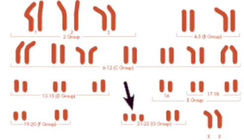
Human cells have 23 pairs of chromosomes (22 pairs of autosomes and one pair of sex chromosomes), people normally have two copies of each chro-mosome, giving a total of 46 per cell. Chromosome 21 is one of the 23 pairs of chromosome in humans, when there is a genetic disorder caused by the presence of all or a third copy of this chromosome, rather than the usual two [12].

2 SOME BIOLOGICAL DEFINITIONS

Figure 1: The genotype variation of Down Syndrome

People with Down syndrome may have some or all of the following phys-ical characteristics: a small chin, slanted eyes, poor muscle tone, a flat nasal bridge, a single crease of the palm, and a protruding tongue due to a small mouth and large tongue. Other common features include: a flat and wide face, a short neck, excessive joint flexibility, extra space between big toe and second toe, abnormal patterns on the fingertips and short fingers [5].

Mouse Model

There are several reasons for using mouse models, among many advan-tages the most important is their striking similarity to humans in anatomy, physiology, and genetics. Over 95% of the mouse genome is similar to our own, making mouse genetic research particularly applicable to human dis-ease. Many of the affected biological systems can not be directly tested in humans, but mouse models can help us do. Besides, mice are small, have a short generation time and an accelerated lifespan (one mouse year equals about 30 human years), keeping the costs, space, and time required to per-form research manageable [9].

Genetically engineered mouse models are useful for elucidating the effects of gene-dosage imbalance on development and contribute to therapies that ameliorate the effects of trisomy 21 [16]. In the early 1990s, the generation of a genetic mouse model for Down Syndrome by Muriel Davisson provided

2 SOME BIOLOGICAL DEFINITIONS

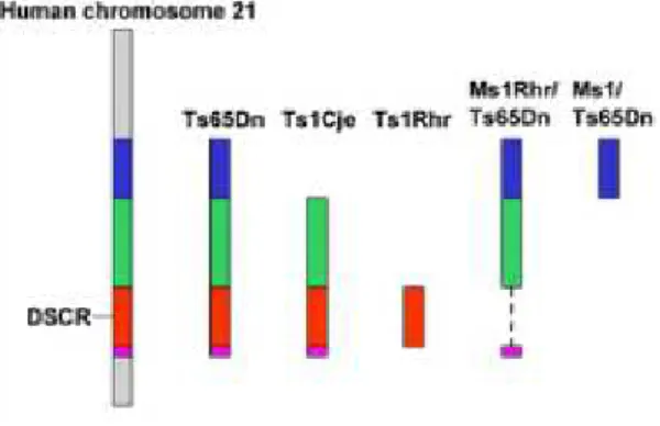
related structural and functional outcomes in mouse and human [13]. The mouse orthologys of genes on human chromosome 21 are found on mouse chromosome 10, chromosome 16 and chromosome 17. A number of Down Syndrome mouse models have(for instance Ts1Cje, Ts3Yah, Ts65Dn, . . . ) segmental trisomy for portions of these chromosomes that have conserved synteny with human chromosome 21 [16].

Figure 2: Comparison of human chromosome 21 with mouse models Figure 2 shows the different genetic mouse stand for different regions of human chromosome 21. If we observe an deformation on mouse model T s65Dn, we know this genetic region of human influence the form of carnio-facial.

Euclidean distance

In Cartesian coordinates, if p=(p1,p2,...,pn) and q = (q1,q2,..., qn) are two

points in Euclidean n-space, then the distance from p to q, or from q to p is given by: d(p, q) = d(q, p) = q (q1− p1)2+ (q2 − p2)2+ · · · + (qn− pn)2 = v u u t n X i=1 (qi− pi)2

2 SOME BIOLOGICAL DEFINITIONS

Here is the three-dimensional Euclidean space : d(p, q) =

q

(q1− p1)2+ (q2− p2)2+ (q3 − p3)2

Landmark

In many biological investigations, the most effective way to analyze the forms of whole biological organs or organisms is by recording geometric lo-cation of landmarkpoints. These are loci that have names(”bridge of the nose”, ”tips of the chin”) as well as Cartesian coordinates. The names are intended to imply true homology(biological correspondence) from form to form. That is, landmark points not only have their own locations but also have the ”same” locations in every other form of the study. The most basic requirement of a landmark is that it can be easily identified and located with accuracy and precision [10] [14].

2 SOME BIOLOGICAL DEFINITIONS

Figure 3 shows the landmarks of mouse skull that is studied by laboratory. The researchers put Landmark to the same place of every mouse. Some of these Landmarks were chosen symmetrically.

3 DATA COLLECTION

3 Data Collection

After we scan a mouse, we have the 3D image with .ply format. A .ply file consists of a header followed by a list of vertices and a list of polygons. The header specifies how many vertices and polygons are in the file, and the (x,y,z) coordinates of each vertex. The polygon faces are simply lists of indices into the vertex list, and each face begins with a count of the number of elements in each list.

The software LandmarkEditor which was developed by IDAV( Institute for Data Analysis and Visualization) and the University of California, Davis, helps us manipulate the .ply file.

Figure 4: The software for capture three-dimensional coordinate of land-marks

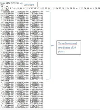
Loading a 3D mouse image, then placing landmark as Figure 3, finally we have the three-dimensional coordinate of these landmarks(Figure 5). In this file, we can see these 39 landmarks’ X, Y and Z axis values.

Then gathering all mice of one model in one file, as Figure 6 showing, we put the 39 landmarks’ information of all the mice who have the geno-type Ts2Yah − Ts65Dn − double in a .txt file, and considering it as a mu-tant group. We have a similar file who gathered the wild type of genotype Ts2Yah _{− Ts65Dn and considering it as a control group. I started analysis} from these two files.

3 DATA COLLECTION

Figure 5: The output of soft-ware LandmarkEditor

Figure 6: The final result for the genotype T s2Y ah − T s65Dn

4 METHODS

4 Methods

We have the basic knowledge to start the analysis of morphometrics of mice. Now I will introduce the method Euclidean Distance Matrix Analysis (EDMA) which is shown by Lele and Richtsmeier [17]. There are some re-lated concepts and a testing procedure for shape differences.

After archiving landmark locations of a three dimensional form, let Xi

be this matrix of landmark coordinates with 39 row and 3 columns(Figure 5): the ith _{row consists of the 3 coordinates of the i}th _{landmark. We can}

calculate Euclidean distances between all possible pairs of landmarks, let F (Xi)denote the formmatrix corresponding to the object with landmark

coordinates matrix Xi and d(i,j) the Euclidean distance between two points

i,j, i,j=1,2,. . . ,39. F (Xi) is a symmetric distance matrix of dimension 39*39

with the form

F (Xi) =          d(1, 1) d(1, 2) . . . d(1, j) . . . d(1, 39) d(2, 1) d(2, 2) . . . d(2, j) . . . d(2, 39) ... ... . .. . . . d(i, 1) d(i, 2) . . . d(i, j) . . . d(i, 39)

... ... ... . .. ... d(39, 1) d(39, 2) . . . d(39, j) . . . d(39, 39)          =          0 d(1, 2) . . . d(1, j) . . . d(1, 39) d(1, 2) 0 . . . d(2, j) . . . d(2, 39) ... ... . .. . . . d(1, i) d(2, i) . . . d(i, j) . . . d(i, 39) ... ... ... . .. ... d(1, 39) d(2, 39) . . . d(j, 39) . . . 0          (1)

We assume that X is some matrix valued random variable. The random variable X consists of the independent X1,X2,. . . ,Xn.

4 METHODS X =                           d(1, 1) d(1, 2) . . . d(1, 39)                                  X1 d(2, 1) d(2, 2) . . . d(2, 39) ... ... . .. ... d(39, 1) d(39, 2) . . . d(39, 39) d(1, 1) d(1, 2) . . . d(1, 39) _      X2 d(2, 1) d(2, 2) . . . d(2, 39) ... ... . .. ... d(39, 1) d(39, 2) . . . d(39, 39) ... ... ... ... ... ... ... ... d(1, 1) d(1, 2) . . . d(1, 39)        Xn d(2, 1) d(2, 2) . . . d(2, 39) ... ... . .. ... d(39, 1) d(39, 2) . . . d(39, 39)

We define equality of form and equality of shape in terms of the matrix valued random variables X and Y , where Y is a matrix of landmark coordi-nates for form Y , Y =(Y1, Y2,. . . ,Ym). We use ”random variable” as shortened

”form of matrix valued random variable”.

Definition 1. Two random variables X and Y are said to have the same form if after proper rotation and translationX and Y are identically distributed. That is:

X == Y P + 1d ktT (2)

for some orthogonal matrix P and a vector t. By identically distributed we mean that the probability distribution functions for X and Y are the same, although particular observations could and would be different.

Definition 2. Two random variables X and Y are said to have the same shape if after proper translation, rotation and scalingX and Y are identically distributed. That is

X == bY P + 1d ktT (3)

for some scalar b > 0, P and t as above. The corresponding definitions in terms of the form matrix are:

Definition 3. Two random variables X and Y are said to have the same shape if

F (X)== cF (Y )d (4) for some scalar c > 0. If c=1, then they have the same form.

4 METHODS

In practice it is difficult to test hypotheses of two distributions (X == Y ),d especially for matrix valued random variables in reason of the sparing data. We give simplified versions of equality of form and shape below in terms of mean form and mean shape. Let E(·) denote the expectation operator. For example, E(X) denotes the average pf the random variable X, or the average form representing a sample of forms.

Definition 4. We say that random matrices X and Y are equal in mean f orm if and only if

E(X) = E(Y )P + 1KtT (5)

for some orthogonal matrixP and a vector t,i.e.,after translation and rotation the means of X and Y are equal.

Definition 5. We say that random matrices X and Y are equal in mean shape if and only if

E(X) = bE(Y )P + 1KtT (6)

for some scalar b > 0, P and t as above, i.e., after translation, rotation, and scaling, the means of X and Y are equal.

Here we are dealing with form matrices F (Xi) and F (Yi) which are

invari-ant under rotation and translation and are therefore identically distributed. We now give the same definitions in terms of form matrices.

Definition 6. Given two random variables X and Y we say that they are equal in mean shape if and only if

F [E(X)] = cF [E(Y )] (7) for some scalar c > 0. By this we mean that two mean forms have the same shape if one form is a scaled version of the other. If c=1 then they are equal in mean shape.

To examine the differences between two average forms we use a matrix of ratios of corresponding linear distances measured on X and Y . We call this matrix the average form difference matrix.

Definition 7. Given two random variables X and Y , we define the average form difference matrix by

D[E(X), E(Y )] = Fij[E(X))] Fij[E(Y )]

where j > i, i=1,2,. . . ,39

(8) when this matrix is a matrix of 1s, we say that the two random variables are

4.1 Testing for Equality of Average Shapes 4 METHODS

4.1

Testing for Equality of Average Shapes

Suppose there are two populations whose shapes we want to compare. Let X1,X2,. . . ,Xn be a random sample of forms from Population X and

Y1,Y2,. . . ,Ym be a random sample from Population Y . The null hypothesis

is that the average shapes of the two populations are equal, which can be expressed using Definition 6, as follows:

H0 : F [E(X)] = cF [E(Y )] for some c > 0

H1 : F [E(X)] 6= cF [E(Y )] for some c > 0

A natural way to test this hypothesis would be to estimate F [E(X)] and F [E(Y )] from the data, calculate the estimate of average form difference matrix D[E(X), E(Y )] using these estimates, and then test whether or not this matrix is ”almost” a matrix of constants or not.

4.2

Estimating the Form Difference Matrix

We will try to find the estimating F [E(X)] and F [E(Y )].The most natural way to estimate F [E(X)] would be to estimate the average coordinates of X,E(X), and then calculate its form matrix. We use generalized procrustes analysis (GPA) [2]. Given X1,X2,. . . ,Xn we apply GPA to get ¯X. This ¯X

is a consistent estimator of E(X). Similarly one can estimate E(Y ) by ¯Y . Here ¯X and ¯Y are coordinstewise averages of X1,X2,. . . ,Xnand Y1,Y2,. . . ,Ym.

F [E(X)] and F [E(Y )] can be estimated by using F ( ¯X) and F ( ¯Y ).

Fij( ¯X) = n X k=1 Fij(Xk) n where j > i, i=1,2,. . . ,39 (9)

F ( ¯_{X) is a symmetry matrix of dimension 39 ∗ 39.}

According to Definition 6, the Form Difference Matrix(FDM) is obtained by:

F DM = F ( ¯X)

4.3 Bootstrap Procedure 4 METHODS

4.3

Bootstrap Procedure

In the following we introduce a bootstrap procedure for estimating the null distribution of the test statistic T . This is based on the permutation test procedure coupled with Bootstrap [1] methodology to reduce the com-putational burden.

For one genotype, Let X1,X2,. . . ,Xn be the sample of mutant group and

Y1,Y2,. . . ,Ym be the control group.

Step 1 Select X∗

i, i=1,2,. . . ,n from X and Yi∗, i=1,2,. . . ,m from Y

ran-domly and with replacement. We have two new samples X∗_=(X∗

1, X2∗,. . . ,Xn∗),

Y∗_=(Y∗

1, Y2∗,. . . ,Ym∗).

Step 2 Use the formula (9) to find the average form F ( ¯X∗) and F ( ¯Y∗) of

X∗ _{and Y}∗ _{respectively.}

Step 3 Calculate T∗ _{by form difference matrix between F ( ¯X}∗) and F ( ¯Y∗),

T∗ ₌ F ( ¯X∗)

F ( ¯Y∗)

the division of the two average form.

Step 4 Repeat Steps 1- 3 B times. A histogram of T∗

j, j=1,2,. . . ,B

estimates the null distribution of T , when H0 is true.

4.4

Testing Procedure

If the observed value of T , i.e., the value calculated with original sample X and Y is in the extreme right-hand tail of the null distribution, we reject H0 at the appropriate level of significance and consider X and Y have

differ-ence form.

Let us see a study introduced by Subhash LeLe [17] of morphological dif-ferences between normal children and those affected with a disease .

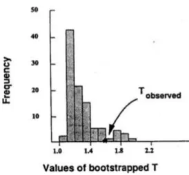
When repeat 100 times the bootstrap procedure we have a distribution of T for the comparison of normal boys and those affected with the disease (Figure 7). Tobs is equal to 1.58 and 10% of the bootstrapped Ts exceed Tobs.

4.4 Testing Procedure 4 METHODS

Figure 7: An example of bootstrapped T

In my case we don not want to know the morphometrics of all landmarks but every landmark, so instead of the histogram of T , we plot another graph. Once obtained T∗

i ,i=1,2,. . . ,B, calculating E(T∗) the average form difference

matrix of T∗

i ,i=1,2,. . . ,B. E(T∗) is a symmetry matrix of dimension 39 ∗ 39.

Eij(T∗) = B X k=1 T∗ k(i, j) B where j > i, i=1,2,. . . ,39 (11)

Because we consider every column of matrix E(T∗_{) as an indication of a}

landmark, drawing up all points (j, Eij(T∗)),for i,j=1,2,. . . ,39, there are 38

values(there is a 0 for the reason the distance between the point itself is 0) for the landmark j. In this graph, we can see how these 38 values scatter around axis y = 1. We also compare the distribution among landmarks.

     1 2 . . . 39 0 E1,2(T∗) . . . E1,39(T∗) E2,1(T∗) 0 . . . E2,39(T∗) ... ... . .. ... E39,1(T∗) E39,2(T∗) . . . 0     

In order to observe which landmarks have more serious deformation, we are trying to define a confidence interval then compare how many values are

4.5 Confidence Interval 4 METHODS

out of the confidence interval. The more values there are, the more serious deformation observed.

4.5

Confidence Interval

Let us find the confidence interval by using control groups of all geno-types. Supposing in total p different genotypes Y1, Y2,. . . ,Yp constitute a set

of Control denoted Y, Y=(Y1,Y2,. . . ,Yp). We define the genotype i which

consisting of mi observations Yi1, Yi2,. . . , Yimi, Yi=(Yi1,Yi2,. . . ,Yimi).

We define a confidence interval of all kinds of genotypes in the way below: Step 1 Pick one of Yij for i=1,2,. . . , p, j=1,2,. . . ,mi and treat the

Eu-clidean Matrix F (Yij) as a reference.

Step 2 Select Y∗

kl, for l=1,2,. . . ,mk from Yk, where k 6= i randomly and

with replacement, calculate F ( ¯Y∗

k) and divide the matrix reference,

V∗ ₌ F ( ¯Y ∗ k)

F (Yij)

repeat this procedure for B times, determine the average matrix of V∗ q,

q=1,2,. . . ,B.

Step 3 Apply Step 2 to all Y∗

k for k 6= i,k=1,2,. . . ,p. We obtain a set of

matrix when matrix Yij is a reference. Find the average of these values, note

aij.

Step 4 Apply Step 1-3 to all observed mice, and obtain a group of aij,

for i=1,2,. . . ,p, j=1,2,. . . ,mi.

Step 5 Observe the distribution of the aij for i=1,2,. . . ,p, j=1,2,. . . ,mi,

then find the 95% interval confidence of all mice.

Another confidence interval is defined for a genotype, it’s similar as we do above in the part Bootstrap Procedure, mixed permutation test and Boot-strap [1] methodology:

In Y=(Y1,Y2,. . . ,Yp), we want to calculate the confidence interval of group

genotype Yi, where i=1,2,. . . ,p,

4.6 Student’s t-test 4 METHODS

Step 2 Select Y∗

ik, k=1,2,. . . ,mi from Yi, and Yjl∗, l=1,2,. . . ,mj from Yj for

j 6= i randomly and with replacement.

Step 3 Use the formula (9) to find the average form F ( ¯Y∗

i ) and F ( ¯Yj∗) of

Y∗

i and Yj∗.

Step 4 Calculate U∗ _{with the form difference matrix,}

U∗ ₌ F ( ¯Y ∗ j )

F ( ¯Y∗ i )

the division of the two average form.

Step 5 Repeat Steps 1- 4 B times. We can obtain a set of U∗

q, q=1,2,. . . ,B,

calculating E(U∗_{) the average matrix of U}∗

q, q=1,2,. . . ,B.

Step 6 Apply Step 1- 5 for all the rest of control groups, collect all these values together and find the 95% interval confidence of them.

Here we apply average of all values instead of matrix, because when we divide one matrix by another, we standardize the distance between two land-marks, then all values are ratio around 1 with the same unit.

4.6

Student’s t-test

Assumptions X1,X2,. . . ,Xn are from sample X ∼ N(µ, σ2), µ and

σ2 _{are unknown.} Hypothesis H0 : µ = µ0 H1 : µ 6= µ0 Test Statistic tobs = ( ¯_{X − µ}0) S√n ∼ tn−1 where ¯X = 1 n n X i=1 Xi, S = s 1 n−1 n X i=1 (Xi− ¯X)2 Critical Region

4.7 Correlation and Simple Linear Regression 4 METHODS

4.6.2 Two-sample t-test Assumptions

The two samples X1,X2,. . . ,Xn1 and Y1,Y2,. . . ,Yn2 have the same variance.

Hypothesis H0 : µ1 = µ2 H1 : µ1 6= µ2 Test Statistic tobs = ( ¯_{X − ¯}Y ) Sw q 1 n1 + 1 n2 ∼ tn1+n2−2 where S2 w = (n1−1)S₁2+(n2−1)S₂2 n1+n2−2 , ¯X = 1 n1 n1 X i=1 Xi, ¯Y = _n1₂ n2 X i=1

Yi stand for the

mean of two samples, s1 =

s 1 n1−1 n1 X i=1 (Xi− ¯X)2, s2 = s 1 n2−1 n2 X i=1 (Yi− ¯Y )2

are the standard deviation of two samples. Critical Region

If |tobs| > tα/2,n1+n2−2, we reject H0, hence, the two samples have different

means.

4.7

Correlation and Simple Linear Regression

The purpose of correlation analysis is exploring the relationships between variables. Two commonly coefficients, the Pearson correlation coefficient and the Spearman for measuring linear and nonlinear relationship respectively [15].

If we have a series of n measurement of X and Y written as Xi and Yi

where i= 1,2,. . . ,n, then the Pearson correlation coefficient r between X and Y is :

4.8 Effect Size(Cohen’s d) 4 METHODS r = n X i=1 (Xi− ¯X)(Yi− ¯Y ) s _n X i=1 (Xi − ¯X)2 n X i=1 (Yi− ¯Y )2

where ¯X and ¯Y are the sample average of the X and Y respectively.

Both correlation coefficients have values between -1 and +1, ranging from being negatively correlated (-1) to uncorrelated (0) to positively correlated (+1). The sign of the correlation coefficient (positive or negative) defines the direction of the relationship. The absolute value indicates the strength of the correlation.

The purpose of simple regression analysis is to evaluate the relative impact of a predictor variable on a particular outcome [15].

A simple regression model contains only one independent variable Xi,

for i =1,2,. . . ,n subjects, and is linear with respect to both the regression parameters and the dependent variable. The model is:

Yi = a + bXi+ ei

where the regression parameter a is the intercept, and the regression param-eter b is the slope of the regression line. The random error term ei is assumed

to be uncorrelated, with a mean of 0 and constant variance.

It is meaningful to introduce the value of the Pearson correlation coefficient r by squaring it; It is the term R-square(R2_{) or coefficient of determination.}

This measure is the fraction of the variability in Y that can be explained by the variability in X though their linear relationship.

R2 = SSregression SStotal = n X i=1 (Yi− ¯Y )2 n X i=1 (fi− ¯Y )2

where SS stands for the sum of squares, fi = a + bXi, and ¯Y is the average

of the observed data.

4.8

Effect Size(Cohen’s d)

We do the test by calculating a p value, which indicates the probability of the null hypothesis being correct. This probability goes down as the size

4.8 Effect Size(Cohen’s d) 4 METHODS

of the effect goes up and as the size of the sample goes up. However, given a sufficiently large sample size, a statistical comparison will always show a significant difference. So here is the idea of effect size.

The most common effect-size measure, as the correlation/ regression co-efficients r (As we talk about before) is actually measures of effect size. The coefficient r covers the whole range of relationship strengths, from no rela-tionship whatsoever (zero) to a perfect relarela-tionship (1, or -1), it is telling us exactly how large the relationship really is between the variables we study and is independent of the size.

As we want do a t-test to compare two means, another common measure of effect size is d, sometimes known as Cohen’s d. This is simply the difference in the two groups’ means divided by the average of their standard deviations. X1,X2,. . . ,Xn1 and Y1,Y2,. . . ,Yn2 are two groups:

d = X − ¯¯ Y s (12) where s = q (n1−1)s2X+(n2−1)s2Y n1+n2−2 and sX = 1 n1−1 n1 X i=1 (Xi− ¯X)2 If n1=n2=n d = X − ¯¯ Y p(s2 X + s2Y)/2 (13)

Figure 8: The indication of cohen’s d

4.9 Software R 4 METHODS

standard deviation; a d of 1 tells us that the two groups’ means differ by one standard deviation and so on.

4.9

Software R

R was created by Ross Ihaka and Robert Gentleman at the University of Auckland, New Zealand. Because of the two ”R” fathers first name begins with R, so it is called R [7]. R is free, but it works as well as the other software, it provides a series of statistical analyses and drawing tools, now it widely used by statisticians, engineers and scientists and become one of the mainstream statistical software.

5 RESULT

5 Result

5.1

Result of EDMA

We took the mouse model Ts2Yah − Ts65Dn as an example. Ts2Yah − Ts65Dn is a mouse model, Ts2Yah − Ts65Dn − double is one kind of its mutant

group. Two groups are compared in this study: a mutant group(Ts2Yah − Ts65Dn − double) with sample size n and a control group of size m. We followed the Bootstrap

Procedure, repeating 500 times to resample the mutant and control groups. We calculated the means of pairwise distance between landmarks for each group, which allowed the generation of the form difference matrix between the two groups(Paragraph 4.3).

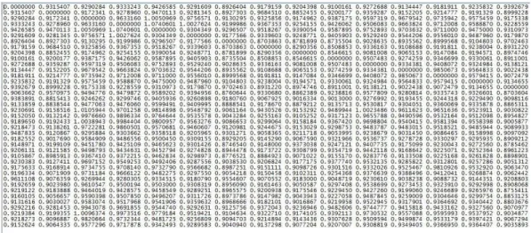
As described in Paragraph 4.4, we calculated the mean of these 500 form difference matrices (because I resampled for 500 times)by formula (11). This procedure allowed us to generate, a symmetry matrix of dimension 39 ∗ 39 (Figure 9), which is essential to analyze the morphometrics.

Figure 9: The form difference matrix of the mouse model Ts2Yah _{− Ts65Dn − double}

To obtain useful information from this matrix, we plot it as described in Paragraph 4.4. In fact, values in every column as represent the average dis-tance from a given landmark relative to every other landmark studied. Every column in the matrix is represented as scattered points, as an indication of the spatial arrangements of any given landmark. For axis x = i, we can see

5.1 Result of EDMA 5 RESULT

landmarks. In this way, the effect in every landmark can be observed.

Figure 10: The graph form difference matrix of the mouse model Ts2Yah _{− Ts65Dn − double}

In this graph(Figure 10), we can see clearly how these 39 landmarks scatter around horizontal axis Y = 1. The value inferior to 1 indicates the mutant mice are smaller on average than the control mice, otherwise, a value superior than 1 indicates the mutant mice has a larger form.

Using this method, we average the spatial position of each landmark in relation to all the others. Deviation of values from 1 indicates a potential shift of the relative position of the landmark.

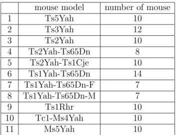
To determine the confidence interval, we used a combined dataset from control groups of different models of mice(Paragraph 4.5). As the overall shape of one model differs from another, we incorporated the variance models to the determination of the confidence interval, which allows for eliminating the variations due to the mice model (false positive) from the deformation caused by genotypic mutations (true positive). The Table 1 shows the control groups and their number of mouse.

5.1 Result of EDMA 5 RESULT

mouse model number of mouse

1 Ts5Yah 10 2 Ts3Yah 12 3 Ts2Yah 10 4 Ts2Yah-Ts65Dn 8 5 Ts2Yah-Ts1Cje 10 6 Ts1Yah-Ts65Dn 14 7 Ts1Yah-Ts65Dn-F 7 8 Ts1Yah-Ts65Dn-M 7 9 Ts1Rhr 10 10 Tc1-Ms4Yah 10 11 Ms5Yah 10

Table 1: Every control group’s number of mouse

Ts5Yah mouse 3940wt 3906wt 3900wt 3935wt 3902wt average 1.0182 1.0133 1.0141 1.0145 1.0043 mouse 3936wt 3917wt 3918wt 3895wt 3946wt average 1.0330 1.0329 1.0271 1.0210 1.0114 Ts3Yah mouse 27wt 72wt 73wt 74wt 79wt 80wt average 0.9643 0.9729 0.9610 0.9617 0.9441 0.9620 mouse 82wt 89wt 94wt 103wt 110wt 111wt average 0.9590 0.9752 0.9532 0.9709 0.9653 0.9555 Ts2Yah mouse 87799wt 87800wt 87801wt . . . average 1.0195 1.0191 1.0463 . . . ... ...

5.1 Result of EDMA 5 RESULT

Using this dataset, we first resampled the group Ts3Yah, then the average distance matrix of group Ts3Yah dividing the distance matrix of 3930wt, repeating this procedure for hundreds of times and obtaining a average form difference matrix; next resampling Ts2Yah dividing the distance matrix of 3930wt. After applying to all mouse models, calculating the average of all these values, we got 1.0182 (Table 2) when 3940wt as reference. We restarted to take 3906wt and then 3900wt of genotype Ts5Yah until the last mouse of the last genotype. We do combinations between one mouse and all the other mouse models, so that we get all the possible values among the mouse models. Finally the list of average could help us find the final confi-dence interval [0.95,1.06]. Figure 12 red line shows this interval’s location of Ts2Yah _{− Ts65Dn − double.}

There is another example shown in Appendix A(Figure 22), there are sel-dom values are located out of this interval, the comparison of these two

geno-type show that the genetic region of human chromosome 21 which Ts2Yah − Ts65Dn − double stand for will effect deformation.

For any given column in the form difference matrix, values which are not in the interval indicate the degree of deformation around this landmark. There are many values out of this interval, we use the number of values which is not in the interval to see how serious the deformation caused by this landmark(Figure 12, the purple numbers below indicate how many values are beyond the confidence interval ). For example the Landmark 9, 38 values are out of confidence interval, au contrary, Landmark 3 has only 16. So the deformation in Landmark 9 is serious than 3.

We took control group of T s2Y ah − T s65Dn as an example to see how we define the confidence interval for it.

Resampling the control group Ts2Yah − Ts65Dn and calculating the av-erage matrix; then finding another control group for instance Ts5Yah, re-sampling and calculating its average matrix; the form difference matrix is defined by these two matrices. Repeating this procedure in order to deter-mine the average of form difference matrix, applying all these steps to the rest of mouse model Ts2Yah, Ts3Yah and so on. At last we pick 95% values among them.

By excluding the impact of the models, we could observe the real effect of a mutation genotype on the deformation. We calculated the confidence

5.1 Result of EDMA 5 RESULT

mouse Ts5Yah Ts3Yah Ts2Yah Ts2Yah- Ts2Yah- Ts1Yah-model Ts65Dn Ts1Cje Ts65Dn CI(2.5%) 0.9131 0.8648 0.9528 0.9356 0.9349 0.9007 CI(97.5%) 1.1299 1.0550 1.1410 1.1003 1.1131 1.0932

mouse Ts1Yah- Ts1Yah- Ts1Rhr Tc1- Ms5Yah model Ts65Dn-F Ts65Dn-M Ms4Yah

CI(2.5%) 0.9102 0.8913 0.9396 0.9062 0.8767 CI(97.5%) 1.1063 1.0870 1.1358 1.10722 1.0499 Table 3: The confidence intervals of every control group

Figure 11: The bar chart of every control group correspondent Table 3

5.2 Result of Correlation and Simple Linear Regression 5 RESULT landmark 8,10 9,17 10,18 11,19 12,20 13,21 23,31

r 0.3878 0.3955 0.5487 0.2887 0.7667 0.7658 0.5553 landmark 24,32 25,33 26,34 27,35 28,36 29,37 30,38

r 0.7973 0.5117 0.6537 0.6666 0.7647 0.7456 0.6825 Table 4: The correlation coefficient of the symmetry right and left landmarks intervals for different mouse models (Table 3) and their variation (Figure 11).Here we take example of a control group: [0.9356,1.1003] is the confidence interval for the model Ts2Yah − Ts65Dn(Figure 12 blue line).

5.2

Result of Correlation and Simple Linear

Regres-sion

To examine the deformation symmetry between right and left sides. I used correlation coefficients between landmarks that are located symmetri-cally (Figure 3).

The correlation coefficients were calculated between seven pairs of sym-metrical landmark(Table 4).

5.3 Result of t-test and Effect Size 5 RESULT

Among these pairs, one pair (Landmark 24 and 32) has the highest corre-lation coefficient, indicating that the variations between these two landmarks are positively correlated (Figure 13).

5.3

Result of t-test and Effect Size

Using the average form different matrix in Figure 9 (still the sample Ts2YahTs65Dn), I performed a one sample t-test by comparing the the con-trol group and mutant group. The average equals to 1 indicates that there is no significant differences between the two groups.

Testing H0 : µ = 1 versus H1 : µ 6= 1

Figure 14: The t-test result T s2Y ah − T s65Dn

The result is summarized in Figure 14 H0 is rejected, meaning that there

is a difference between the control and mutant group.

Next I applied a two sample t-test to assess if the deformation caused by mutation is more significant than the deformation results from model vari-ations. To find the confidence interval of Ts2Yah − Ts65Dn(Paragraph 4.5 and Paragraph 5.1), we resampled the control group of Ts2Yah − Ts65Dn, then divided its mean Euclidean matrix by an other resampling control group, this was repeated for hundreds of times until a mean form matrix was gen-erated. The procedure was applied to all the other control groups. By doing this, we obtained a mean form matrix for each control group,which allowed for the calculation of a final mean form matrix for all control groups, denoted Ma. To test if the mean of Ma is equal to the mean form difference matrix

of Ts2Yah − Ts65Dn − Double(Figure 9), I used the following: Testing H0 : µ1 = µ2 versus H1 : µ1 6= µ2

5.3 Result of t-test and Effect Size 5 RESULT

Figure 15: The t-test result of T s2Y ah − T s65Dn and the mean form differ-ence matrix

As shown in Figure 15, the test is significant in level of 5%, which means the influence of the mutant group Ts2Yah − Ts65Dn is more significant than the variation observed between the mouse models. Nevertheless, as the dataset is relatively large, it is always possible to a false significant re-sult. Using the formula (12) and (13), I obtained a value of 3.9763 for cohen’s d, indicating that the two matrix’s means differ by almost four standard de-viations.

I also calculated the cohen’s d of these two matrices by column in order to observed how these landmarks affect the deformation.

Figure 16: The 39 landmarks’ Effect Size result of Ts2Yah − Ts65Dn Comparing Figure 12 with Figure16, for cohen’s d, the Landmark 15 is large and many values surpass the confidence interval. By contrast, the Land-mark 4 has less number of outlined values that are compact distributed below

the interval. Therefore We can consider that with the genotype Ts2Yah − Ts65Dn − Double, the Landmark 15 showed a more serious deformation than Landmark 4.

6 DISCUSSION

6 Discussion

Here we show how the Euclidean distance matrix-based approach for com-parison of shapes suggested by Lele and also the comcom-parison of two groups statistically. Then trying to identify those areas where the differences are prominent. For this method, if we can have more Landmarks, the more ac-curate result we will get. So here comes the problem to get more Landmarks’ information. I also did much research about .ply file so that the Landmark could be put automatically and we could put as many landmarks as we want. Unfortunately it is just can be done manually, because the data stock in .ply file is not matched, for instance, the vertex 1 in file 1 is not the same in file 2.

As mentioned before, the t-test could always get a signification result be-cause the size of sample was large enough so we used Effect Size to study the deformation.

For Simple Linear Regression, there existed aberrant values(sometimes they appear in pairs, because the distance from Landmark i to j is equal to Landmark j to i), in this way, the relationship would be effected. So when we want to study the symmetry, we should combine the simple linear regression with the number of values which are out of confidence interval and how they distribute(Figure 13).

7 CONCLUSION

7 Conclusion

During my internship, I learned a new statistical method EDMA (Eu-clidean Distance Matrix Analysis) which is widely used in the field of biol-ogy, medicine for morphometrics. With this method, I could compare two groups’ shape. I determined the confidence interval for all control groups and for every control group in order to observe if the deformation caused by genotype is more serious than the difference caused by mouse model. Then we could find which genotype will lead to the deformation.

I strength my ability of programming on software R, all my project real-ized on it, in my laboratory, before we do the analysis in different software separately, and now with my new program, getting the new dataset and graphs become easier. Besides, when I tried to collect data from the image I learned a lot about how to read and write a file especially the format .ply with software matlab.

REFERENCES REFERENCES

References

[1] Efron B. The Jackknife, the Bootstrap and Other Resampling Plans. SIAM, 1982.

[2] Goodall C. Procrustes method in the statistical analysis of shapes. J.R.Stat.Soc.Ser.B, (53):285–339, 1991.

[3] F.B. Churchill. William Johannsen and the genotype concept. Springer, 1974.

[4] Michel E. Weijerman J.Peter de Winter. The care of children with down syndrome. Springerlink, (169 (12)):1445–52, 2010.

[5] Frank J. Domino. The 5-minute clinical consult 2007. LWW, 2007. [6] Howard G.Tucke. The Annals of Mathematical Statistics 30, volume 30.

Institute of Mathematical Statistics, 1959.

[7] Kurt Hornik. The r faq: Why is r named r, 2008.

[8] W. Johannsen. The genotype conception of heredity. The American Naturalist, 45(531):129–159, 1911.

[9] The Jackson Laboratory. Advantages of the mouse as a model organism. [10] Fred L.Bookstein. Morphometric Tools for Landmark Data: Geometry

and Biology. Cambridge University Press, 1991.

[11] RC; Haugsand TM; Ulvestad IH; Emilsen NM; Hansen B; Cardenas YE; Skøld RO; Thorsen AT; Davidsen EM Malt, EA; Dahl. Health and disease in adults with down syndrome. Tidsskrift for den Norske laegeforening : tidsskrift for praktisk medicin, ny raekke, (133 (3)):290– 4, 2013.

[12] D Patterson. Molecular genetic analysis of down syndrome. Human genetics, (126(1)):195–214, 2009.

[13] Moran TH Wohn A Kitt C Sisodia SS Schmidt C Bronson RT Davis-son MT. Reeves RH, Irving NG. A mouse model for down syndrome exhibits learning and behaviour deficits. Nat Genet, (11(2)):177–84, 1995.

[14] Elfert PC et al. Richtsmeier JT, Paik CH. Precision, repeatability, and validation of the localization of cranial landmarks using computed

to-REFERENCES REFERENCES

[15] Kelly H.Zoum; Kemal Tuncali; Stuart G. Silverman. Correlation and simple linear regression. Published online Radiology, 2003.

[16] Ratliff TS Reeves RH Richtsmeier JT Starbuck JM, Dutka T. Over-lapping trisomies for human chromosome 21 orthologs produce similar effects on skull and brain morphology of dp(16)1yey and ts65dn mice. Am J Med Genet Part A, (9999):1—10, 2014.

[17] Joan T.RICHTSMEIER Subhash LELE. Euclidean distance matrix analysis: A coordinate-free approach for comparing biological shapes using landmark data. American Journal of Physical Anthropology, (86):415—427, 1991.

A. FIRST APPENDIX

Appendix A

First appendix

Figure 17: The 22 Landmarks of mouse mandibular

Figure 17 (similar to Figure 3) is the 22 Landmarks of mouse mandibular. Using these 22 Landmarks we can explore the morphometric.

Figure 18: The form difference matrix of the mouse model (mandibular) Ts2Yah _{− Ts65Dn − double}

The form difference matrix for mandibular (Figure 18 similar to Figure 9) is a symmetry matrix of dimension 22 ∗ 22. Then we plot this matrix by column.

Figure 19 (similar to Figure 12) is the graph corresponding the matrix in Figure 18, the all control groups’ confidence interval of mandibular is [0.93, 1.057]. There are still many values are out of the interval, that means this

A. FIRST APPENDIX

Figure 19: The graph form difference matrix of the mouse model(mandibular) Ts2Yah _{− Ts65Dn − double}

genotype will cause serious deformations.

We can also define the confidence interval for every genotype, then we have the result showing in Table 5 and Figure 20 .

If we plot the scatter diagram between two symmetry Landmark, we ob-serve a linear relationship. Figure 21 is the Linear Regression corresponding the Table 4, we can see the relationship between the symmetry landmarks.

Figure 22 is an example showing that there are not always as many val-ues out of the confidence interval as Figure 12. Here we take the confidence interval of all control group [0.95, 1.06] as before. So we can consider that the genotype Ts2Yah has less effect than genotype Ts5Yah-Ts65Dn-Double in phenotype (skull’s deformation) of Down Syndrome, the corresponding ge-netic region of human chromosome 21 effect not as much as Ts5Yah-Ts65Dn-Double.

A. FIRST APPENDIX

mouse Ts5Yah Ts3Yah Ts2Yah Ts2Yah- Ts2Yah- Ts1Yah-model Ts65Dn Ts1Cje Ts65Dn CI(2.5%) 0.8690 0.8372 0.9303 0.9610 0.9542 0.9384 CI(97.5%) 1.1173 1.0604 1.1339 1.1599 1.1178 1.1395

mouse Ts1Yah- Ts1Yah- Ts1Yah- Ts1Rhr Tc1- Ms5Yah model Ts65Dn-F Ts65Dn-M Ts1Cje Ms4Yah

CI(2.5%) 0.9455 0.9230 0.8831 0.9225 0.7530 0.8797 CI(97.5%) 1.1502 1.1341 1.1125 1.1327 1.1270 1.0689

Table 5: The confidence intervals of every control group(mandibular)

Figure 20: The bar chart of every control group (mandibular) correspondent Table 5

A. FIRST APPENDIX

Figure 21: The symmetric Landmarks’ Simple Linear Regression of Ts2Yah _{− Ts65Dn − Double}

B. SECOND APPENDIX

Figure 22: The graph form difference matrix of the mouse model (skull) Ts2Yah

Appendix B

Second appendix

Bootstrap Procedure

X = (X1, X2, . . . , Xn) is the sample from a population with distribution

function F (x), θ is the parameter we are interested in, ˆθ = ˆθ(X1, X2, . . . , Xn)

is the estimator of θ.

Supposing the distribution F is unknown,x = (x1, x2, . . . , xn) is the

ob-servations from the sample X = (X1, X2, . . . , Xn) of F , Fn is the empirical

distribution. When n is large enough, according to Glivenko - Cantelli the-orem [6], Fn has an approximating distribution to Fn.

We pick x∗

i, i=1,2,. . . ,n from x randomly and with replacement. We have

a new sample x∗_=(x∗

B. SECOND APPENDIX

We repeat this procedure B times and get ˆθ∗

i, for i = 1, 2, . . . , B, we can

con-sider θ¯ˆ∗ ₌ 1 B B X i=1 ˆ θ∗ i is a new estimator of ˆθ

The Simple Linear Regression

Suppose there are n data points (Xi, Yi), i = 1,2,. . . ,n. The model is :

Yi = a + bXi+ ei

we use linear least squares method to estimate the unknown parameters. This method minimizes the sum of squared vertical distances between the observed responsesn the dataset and the responses predicted by the linear approximation. we are trying to find:

min Q(a, b) for Q(a, b) =

n

X

i=1

(Yi− a − bXi)2

By using calculus, we can obtain the estimators of a and b. ˆb = Pni=1(Xi− ¯X)(Yi− ¯Y )

Pn

i=1(Xi− ¯X)2

ˆ