ADAPTIVE X-TRACKING FOR LINEAR SYSTEMS WITH
HIGHER RELATIVE DEGREE
-THE CONTINUOUS ADAPTATION CASE
Eric Bullinger * Frank AllgSwer ** Institut fiir Automat&, ETH Ziirich, 8092 Ziirich, Switzerland {bullinger,allgower}Oaut.ee.ethz.ch
Fax.: + 41 1 6%’ 1211
Keywords: lambda-tracking, adaptive control, high-gain, robust stability, universal stabilization, observers.
Abstract
This paper presents a simple adaptive controller which universally achieves so-called X-tracking for linear systems where only little structural information about the system to be controlled is needed. The paper extends previous results to the case of systems with higher relative degree. Stability and convergence of the adaptation is proven for tracking arbitrary but sufficiently smooth reference trajec-tories. The design of the controller is very simple and in-tuitive and only few parameters have to be tuned. The ro-bustness is increased by the introduction of a dead-zone in the adaptation, whose width X can be chosen by the user. In this paper a continuous adaptation law is used as op-posed to the discrete law suggested in earlier papers. The’re are several advantages in using a continuous adaptation: Besides displaying a simpler structure the necessary gain to achieve the control goal will also be significantly lower in general. To demonstrate the performance the controller is applied to the model of a ball and plate experiment.
1 Introduction
A popular method for the robust stabilization of ctrol systems is adaptive conctrol. On the one hand, on-line identification techniques are used for tuning the con-troller (see (Ast95; Nar91) for a survey). In non-identifier-based adaptive control, on the other hand, the controller is directly tuned without estimating the parameters of the plant, usually by increasing it as long as the control ob-jective has not yet been achieved (see (Ilc91) for a sur-vey of earlier works). The first, rather complicated non-identifier-based controller was proposed in 1978 by Feuer and Morse (Feu78). In the mid-80’s several authors im-proved and simplified the adaptation and the controller structure, see (Ilc91) for a list of references. These
con-trollers achieve stabilization via adapting a gain continu-ously or in a step-wise manner. The latter has the draw-back there is that the height of the steps has to grows expo-nentially. Usually, the gain adaptation reduces to increas-ing the gain as long as the control objectives, for example stabilization, have not been achieved.
To increase the robustness especially when output noise is present, a dead-zone (of width X) in the gain adapta-tion is introduced in (Mi191; Ilc94). This is usually called X-stabilization or X-tracking as the objective is to control the output or the tracking error no longer to zero but to a X-neighborhood of zero. Thus, an output error of am-plitude smaller than the width of the dead-zone does not increase the adaptation parameter. While in (Ilc94) a con-tinuous adaptation is used for systems of relative degree one, (Mi191) and later (Bu199b) who are dealing with the higher relative degree case need an adaptation parameter that is increasing in a step-wise manner.
Our contribution is to propose a simple adaptation scheme allowing X-tracking with a continuously increasing adaptation parameter for any minimum-phase linear sys-tem with known relative degree while keeping the simplic-ity of the controller. This leads to a simple, robust con-troller that does not need the discontinuities in the adap-tation parameter and the tracking error is guaranteed t,o converge to the interval [0, X]. Another approach for treat-ing the higher relative degree case with a continuous adap-tation has recently been proposed in (Ye99), but due to the fact that there the X-tracking controller is derived via backstepping, the controller design and the resulting con-troller are more complicated.
To demonstrate the applicability of the X-tracker the controller is applied to the model of a ball and plate labo-ratory setup.
The paper is organized as follows. After stating the system class and explaining the structure of the controller in Section 2, the theory and an outline of the proof are presented in Section 3. Section 4 presents the example.
2 Preliminaries System class
We consider linear systems with known relative de-gree r > 1, having one input and one output and stable zero-dynamics, therefore being stabilizable and detectable. They can be described by the differential equation
k(t) =
AZ(~) + bu(t), A E IF”“, (la) y(t) = cz(t), z(t), b, CT E Iw” (lb) withCA% = 0 for i = 0,. . . , T - 2 (2a)
CA‘-lb = g 2 ij > 0, G’b)
d e t [‘In: A i] # 0 for all s E ?J+ (2c) where (2a), (2b) are the relative degree conditions and (2~) guarantees minimum phaseness.
Objective
The control objective is to track a reference signal ylref (.) asymptotically while tolerating a tracking error smaller than a user-defined X. All states should remain bounded, i.e. x E L,. yref (.) is in I&“+, the set of all bounded func-tions that are absolutely continuous on compact subinter-vals and whose r first derivatives are essentially bounded. This set includes almost all practically relevant signals.
For this an adaptive output-feedback controller is de-signed in the state-space. It consists of an adaptive high-gain observer and an adaptive high-high-gain controller, both described in the following.
Observer
The observer is an adaptive version of the high-gain observer introduced by Nicosia and Tornambit (Nic89) as in (Bu197). A state-space representation is
i(t) = a&%(t) + &e(t) e(t) = y(t) - yTef(t) with li: E Iw’ and
- -p,-1 6 1 0 -pr_‘J .K? 0 1 a,= : . . , &,= -Pl.cl 0 0 1 -PO. K’ 0 0 0
(34
WI
PT-1.
fc
PT.-2 .K2 p1 . d-1 PO. /ST _ Note that if the parameters pi are chosen such that s” + CIIi pisi is a Hurwitz polynomial, then for any positive^ value of the observer gain n, the spectrum of A, lies in the open left half plane, ~(ff,) c C_ and the observer dynamics are stable. No further knowledge of the model besides that of the relative degree is needed for the observer design. The observer gain K is adapted according to the adaptation law described below.(4)
ControllerThe controller is an observer-state feedback where
21 = -qk2,
4rc = [Qo+, “. , qr-1 .k]
The parameters qi are chosen such that sT + g C’izi qis’ is a strongly Hurwitz polynomial. Then for any positive value of the controller gain Ic, the spectrum of A - bq, lies in the open left half plane. Of the model, only the relative degree and a lower bound of the high-frequency gain are needed for the controller design. The adaptation law for the controller gain k is described below.
Gain Adaptation
The adaptation for the observer gain IC. and the controller gain Ic is chosen in such a way that the gains are increased as long as the amplitude of the tracking error e is larger than the user-defined bound X from the control objectives.
Let, for X > 0, y > 0, Ic(0) = Ic0 > 0, i(t) =dx(e(t), k(t))2; dx(e, k) = 6
{
F’-’ for le’ “’ for lel< X. (5) In order to guarantee the achievement of the objectives the observer gain K has to grow sufficiently faster than the controller gain k for large It’s. For simplicity, we choose as a simple case K = Ic2.
This adaptation law ensures a monotonical increases of the observer and controller gains.
In Section 3 we need the following definition.
Definition 1 A poZynomiaZp(s) = .sr+Ci$ pisi is called strongly Hurwitz if p(s) is a Hurwitz polynomial and there exists a symmetric, positive definite matrix P such that the companion matrix 0 1 A= ; “.. I I 0 1 -po . . . . . -p,1
satisjies for 9, = diag{l, 2, . . . , r} the inequalities
AT.P+P.A<O (6a)
9,.P+P.QT >o. (6b)
A matrix with a strongly Hurwitz characteristic polynomial will be called strongly Hurwitz.
Remark 1 As shown in (BulSSc), the strongly Hurwitz condition is not a restrictive assumption.
Remark 2 Systems with CA’-lb = g 5 ij < 0 instead o,f (2b) can easy be treated by changing the sign of the con,-troller.
3 Results
As stated in the following theorem we can prove that combining the adaptive observer (3) with the adaptive con-troller (4) and using the adaptation law (5) with IC. = k2 to close the loop of an arbitrary system of class (1)) (2) yields that the tracking error asymptotically converges to the X-strip, that the adaption converges, that all states remain bounded and that no finite escape time can occur.
Theorem 3 If fOT all q >_ ij, sT + ~~~~pisi and sT +
4 CLli qisi are strongly Hurwitz polynomials then the ap-plication of the X-tracker (3), (4), (5) with FC = k2 to any stabilizable system of the class (l), (2) and to any reference signal yref
(.)
E W’)” results in a closed-loop system which, independently of the initial values Z(O) E Iw”, i(0) E IF, k(0) > 0 has a unique solution which exists on the whole half axis t E [0, 00) and, moreover,b) limt+oo dist()e(t)], [0, A]) = 0.
Remark 4 Theorem 9 states that for any linear system with known relative degree and lower bound of the high-frequency gain, a X-tracking controller can be designed with
the guarantee that all states and adaptation parameters re-main bounded and that the tracking error y - yref asymp-totically converges to the X-strip. The width of this strip is a parameter which can be chosen by the user and will usu-ally depend on the specifications, on model uncertainties and on the quality of the measurement.
Remark 5 The motivation for such an observer-based controller comes from the fact that for fixed adaptation pa-rameters k and IF, the transfer function from y to gi, the i-th state of the observer,
&(s) ZI
si-1
1-(
(a)” +. . . + (;)n-i+lpi_l
(a)”
-I- (;)+lp1+ . . . +p, ) y(s), is at ((low” frequencies, i.e. for small (a), approximately a series of differentiators,?i(S) M Siel$/(S)
with a band width proportional to the observer gain. Thus, the observer states approximate the derivatives of the output y Therefore, the controller is approximately a PD...Dr-1 controller:
T-l l--l
u(s)
22-kc
q&r-l-iy(s) = -k’ c qi ( ;)Zy(s).i=O i = O
Proof
T h e f o l l o w i n g l e m m a , p r o v e n i n (Bu199b) will be used in the proof of Theorem. 3.
L e m m a 6 ( N o r m a l f o r m ) Every stabilizable linear sys-tem (A, b, c) of order n and relative degree r as given in (1)
and (2) is s i m i l a r t o t h e f o l l o w i n g s t a t e space
representa-A 6
tion (A,&,C):
H-l
s:o=-C
where a(&~) C @_, a(&) C c.- and the stars indicate for real entries. All other entries are zero.
Proof (of Theorem 3)
Outline of the Proof. We will prove Theorem 3 in four steps. First, it is shown that k cannot go to infinity on the maximal time interval where all states remain bounded. Then, it is proven that the solution of the differential equa-tions exists for all times and thus that the maximal time interval of existence of the solution is infinite and that there are no peaking effects. A consequence of the first two steps is that the controller gain k converges. In the third part boundedness of the observer states 2 and thus of the plant input ‘1~ as well as boundedness of the plant states x is shown. The proof concludes by showing that the tracking error converges to the X-strip.
1) Boundedness of the adaption parameters. By Lemma 6, we may assume that the system is given in the normal form (7). The nonlinear closed-loop system (7))
(3), (4) and (5) is of the form
2 = Ax - bq,?, Z(.O) = XI-J E IR” (W & = A,li: + 6,e, 2(O) = 2’0 E Iw’ (8b) k = dx(e, k)2, k(0) = ko > 0, (3~)
e = cx - yref. (3d)
Using the coordinates gCT = [c’, zT, GT] where ET =
[Xl - Yref, x2 - Yref, ..‘, xr - Y,,f(r-‘)] denotes the tracking error and its derivatives, x = [xT+r, . , cc,,] are the uncontrollable, but stable states and those of the zero-dynamics, [S&+1, . . . , ~~1 in (7), and e =
[Xl,... ,GIT - 5 E Et’ is the observer error, the closed
loop (8) can be written as
% = i5z - ByTef =: f(g,t). (9) With
T g=K-l tT,
[ ZT, @ST
1
(10)w h e r e K = diag{Ki,, Im, Kz}, K, = diag{lc, Ic2, , kT} and setting K. = k2, the closed-loop differential equation is
with 9 = diag[Ql,,O,, qT], Qr = diag[l, 2,. . . ,r], A = diag{A,,A,,A,} = diag{~l,,I,,Ic21;.}, 2 =
I
A 1 -_and 5 = k-(T-l)ep[~O, . . . , c+~, I], YrTef = 1Ylre.f , hef , . . . , Y!$], qi = qi . g. e, is the r-th unit vector and A E IR(“-‘)x(“-‘) is Hurwitz as A is block-triangular with the stable matrices 1122, _&3 on the diagonal.
By assumption, the matrices 222 = A,
are strongly Hurwitz. Therefore, there exist unique sym-metric, positive definite solutions PI, P2, P3 of the Lya-punov equations
zzPi + Pixii = -Qi i = 1,2,3, Pi*, + q‘,Pi > 0 i = 1,3.
Wa) (lib) for some matrices Qi > I, i = 1,2,_3. The state space partitioning of 2 and l? into Zi and Bi respectively with i = 1,2,3 corresponds to the one for 2.
Boundedness of the adaptation parameter is done via contradiction. Due to lack of space, this part of the proof is not shown here but can be found in (Bu199a).
2) Global existence of a unique solution. Applying the boundedness of k to (9), it can be seen that there exist
constants c, d, s.t.
If( I c[lZjl + d and f(.) E Cl. Thus, s(t) exists for all t E IR (Ha180).
3) Boundedness of the observer states. As k(.) is bounded, dx(.) E &(O, co). From that, (5) and the H6lder inequality follows that
y-‘k’(.)dx(.) E Ls(0, m).
Combining this with
le(.)l - r-‘k’(.)dx(e(t), k(t)) E J%(O) m), yields that
le(.)l = Ie(.)I - y-‘k’(.)dx(.) +y-'k'(.)dx(.)
PM (12)
Lco(O,m) ELZ(0,~)
Defining t(t) = Knox, a = a,=,, & = hK.=l, (8b) is transformed to
6 = k2& + k2be - :2Y,,$ define a, = k&a, ff2 = a - a,, a3 = -2$Q,
i = a,< + a,[ + &< + k2&e. (13)
Al is a constant Hurwitz matrix and there exist to >
0, MI > 0, M2 > 0, M3 > 0 such that
lIA2(t)ll
L
Ml
for
all t > to,
J
m Ilff,(Wt = ll*ll log(k =: ~5f2, toAd3 = 11611, and
M4,p > 0 : l/e A(t-to) 11 5 J,f4e-mYwo)y~ > to,
Variation of Constants, see e.g. (Be153), to (13) yields
Il~(t)II
5 M4e-p(t-t0)ll~(t0)l~ +J
t M4e-p(T-to)(ll-42WII + lL43(~)ll + &M+~l) d7
5 ~4115(to)ll + +h + M2)
+ iKJ&k&
Jtot
le(7)le-L1(T-to)d7.Combined with (12), this yields that [(.) is bounded (Des75), and by the boundedness of k it follows that
2(.) E &(O, m) a n d u = -SkS?(.) E L,(O,co). (14) 4) Boundedness of the states of the plant. Since (c, A) is detectable, there exists some k E Cnxl such that a(A - kc) c C-. Now consider the observer
& = A53 + bu + kc(a:-5) = (A-kc)% + bu + k(e-y,,p). By (12), (14), and the exponential stability of (A - kc) it,
holds that 2 E L,. Exploiting exponential stability of $(z - 2) = (A - kc)(a: - 5)
again and boundedness of Z yields z(.) E L,(O, co) and also e(.) = cZ(.) - yref(.) E L,(O, 00).
5) Convergence of the tracking error. It remains to show b). For this we prove that lirntqco dx(e(t), k(t)) = 0. Since e(.) and Ic(.) are bounded it follows that ,&(.) = dx(.)” E L,(O,co). F r o m i: = c[Az - bq,ck] - GTef a n d previous results we conclude e(.) E L,(O, oo). NO W
&t)2 = 2&(t) (
e(t)ic(.)
-l4t) I - r;&(t)) E -Lo(O, 00)
and hence dA(.)2 is uniformly continuous. This, to-g e t h e r w i t h dx(.)” E &(O, m) y i e l d s , b y BarbMat’s Lemma (Bar59) that limt+.w dA(t)2 = 0.
This completes the proof. n
4 E x a m p l e
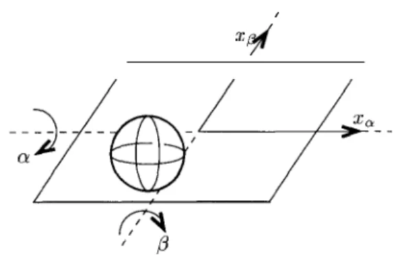
To demonstrate the applicability of the proposed X-tracker the controller is applied in simulation to the iden-tified model of a ball and plate laboratory setup (Her97). The system is depicted in Figure 1. The objective is to make a steel ball follow a user-defined trajectory by ap-plying voltages to the motors controlling the angles of a plate that can be rotated about two axis (a and ,D). The dimensions are approximately 80 cm x 80 cm for the plate and the radius of the ball is 5cm The maximal angles of the plate are about 6” for each of the axes a, /3.
Following (Her97) the ball and plate system can well be approximated by two linear, decoupled systems of the form
Xi(S) =
ai W(S), ai > 0, bi > 0, Ci > 0s2(s2 +
his + Ci) i=cy,/3due to the fact that the maximum angles are small. There-fore, this system with two inputs and outputs can be treated as two decoupled single input single outputs sys-tems, for which controllers can be designed independently. xa and ~0 are the ball positions relative to the plate in di-rection of the cr and p axis, respectively (see also Figure 1). Thus, the dimension of each system and the relative de-gree are both 4, implying that the system has trivial zero dynamics and is thus minimum phase. We assume that the high frequency gain, here equal to ai, is larger than 20. For the controller design we make no further assumptions about the model. In particular, we assume that the values ai, bi, ci are not known. The parameters of both controllers have been chosen as the following strongly Hurwitz poly-nomials: parameters p and q are such that the poles of the respective polynomials lie at 1,2,3,4 for the observer and for the controller, both for a controller gain of 1. For both axes, the controller parameters are chosen to be Ice = 1, y = 1000, X = 1 cm. The reference trajectory consists of a circle with radius of 20 cm for the first minute, 10 cm for the second, and 15cm for the last. The observer and the model are both initialized at the center of the plate, i.e. at zero.
I X
4
Figure 1: Sketch of the Ball and Plate system.
For the simulations, model (4) with the numerical val-ues identified in (Her97) as a, = 34.2, b, = 16~~‘, c, = 400~~~ respectively ap = 37.9, bp = 19s-l, co = 64Os-” has been used to represent the plant. Again, these paran-eters were not used for the controller design.
The result can be seen in Figure 2. In Figure 2.a an xy-plot of the ball’s trajectory over three minutes starting at the origin is shown. After the transient the ball follows quite well the reference trajectory, depicted by plus signs. In Figure 2.b the tracking error is depicted. It can be seen that it is slowly decreasing towards the X-strip. There, it keeps oscillating. There are fast increases of the controller gain during the first seconds and then smaller ones each time the corresponding tracking error leaves the X-strip, as shown in Figure 2.~.
5 C o n c l u s i o n s
[Section] In this paper a high-gain adaptive controller for linear, minimum-phase systems of arbitrary, but known relative degree is presented. This is the first step in the di-rection of X-tracking of high relative degree nonlinear sys-tems. The assumption of knowledge of a bound on the high frequency gain should be removed in the future. Future research will focus on nonlinear systems.
A c k n o w l e d g m e n t
This work was supported by a British Council/ Schweiz-erischer Nationalfond grant. The authors thank Achim Ilchmann of the School of Mathematical Sciences, Univer-sity of Exeter, UK for many helpful comments and discus-sions, and George Weiss of the Centre for Process Systems Engineering, Imperial College of Science and.Technology, UK for pointing out the simple proof in Step 4.
[Ast95] Astr6m K., Wittenmark B., Adaptive Control, Addison-Wesley, Reading, MA, second edition (1995).
[Bar591 Barbglat I., Yystemes d’Gquations diffkrentielles R e f e r e n c e s
I I
-0.2 -0.1 0.1 0.2
(a) Ball position and reference.
’
-0.1 , / -0.2 0 _ e -a ---eb
60 120 180 (b) Tracking errors. 2 I/ 7mm ---_ __ _--- _______. , (c) Controller gains.Figure 2: Ball and Plate with X-tracking control.
[Be1531
[Bu197]
[Bu199a]
d’oscillations non linkaires” , Rev. Math. Pur. Appl., 4:267-270 (1959). Acad. Republ. Popul. Roum.
Bellman R., Stability Theory of Differential Equations, International Series in Pure and Ap-plied Mathematics, McGraw-Hill, New York
(1953).
Bullinger E., Allgijwer F., “An adaptive high-gain observer for nonlinear systems”, in: “36th Conf. on Decision and Control, San Diego, USA”, pp. 4348-4353 (1997).
Bullinger E., Allgijwer F., “Adaptive X-tracking for linear systems with higher relative de-gree - the continuous adaptation case”,
Tech-[Bu199b] [Bu199c] [Des751 [Feu78] [Ha1801 [Her971 [Ilc91] [Ilc94] [Milgl] [NarSl] [Nic89] [Ye991
nical Report 99-08, Automatic Control Lab-oratory, Swiss Federal Institute of Tech-nology (ETH), Ziirich, Switzerland (1999). http://www.aut.ee.ethz.ch/cgi-bin/reports.cgi. Bullinger E., Ilchmann A., Allgiiwer F., “Piece-wise constant high-gain adaptive X-tracking for higher relative degree linear systems”, in: “Proc. 14th IFAC World Congress”, (1999). Accepted. Bullinger E., Kraus F., “Solvability of certain matrix inequalities”, Technical Report 99-06, Automatic Control Laboratory, Swiss Federal Institute of Technology (ETH), Ziirich, Switzer-land (1999). http://www.aut.ee.ethz.ch/cgi-bin/reports.cgi.
Desoer C., Vidyasagar M., Feedback Systems: Input-Output Properties, Academic Press, New York (1975).
Feuer A., Morse A., “Adaptive control of single-input, single-output linear systems”, IEEE
Trans. Automatic Control, 23(4):557-69 (1978). Hale J., Ordinary Differential Equations, Krieger Publishing, Malabar, Florida, second edition (1980).
Hermann O., Regelung ekes “Ball & Plate” Systems, Diplomarbeit, Institut fiir Automatik, ETH Ziirich, Switzerland (1997).
Ilchmann A., “Non-identifier-based adaptive control of dynamical systems: A survey”, IMA Journal of Mathematical Control and Infornw-tion, 8:321-366 (1991).
Ilchmann A., Ryan E., “Universal X-tracking for nonlinearly-perturbed systems in the presence of noise”, Automatica, 30(2):337-346 (1994). Miller D., Davison E., “An adaptive controller which provides an arbitrarily good transient and steady-state response”, IEEE Trans. Automatic
ControZ, 36(1):68-81 (1991).
Narendra K., “The maturing of adaptive con-trol”, in: “Foundations of Adaptive Concon-trol”, edited by P. KokotoviC, pp. 3-36, Springer-Verlag, Berlin (1991).
Nicosia S., Tornambk A., “High-gain observers in the state and parameter estimation of robots hav-ingelastic joints”, Syst. ControZLett., 13(4):331-337 (1989).
Ye X., “Universal lambda -tracking for nonlinearly-perturbed systems without re-strictions on the relative degree”, Automatica,