Spectral generation and control of linear and nonlinear self-accelerating beams and pulses.

(1)

i

Université du Québec

Institut National de la Recherche Scientifique (INRS) Centre Énergie, Matériaux et Télécommunications (EMT)

SPECTRAL GENERATION AND CONTROL OF LINEAR AND

NONLINEAR SELF-ACCELERATING

BEAMS AND PULSES

Par

Domenico Bongiovanni

Thèse présentée pour l’obtention du grade de Philosophiae doctor (Ph.D.)

en Énergie, Matériaux et Télécommunications (EMT) Varennes, Québec, Canada

Jury d’évaluation

Président du jury et Prof. FrançoisVidal

Examinateur interne INRS-EMT, Québec, Canada

Examinateur externe Prof. Mohammad Mojahedi

University of Toronto, Ontario, Canada

Examinateur externe Prof. Michel Piché

Université Laval, Québec, Canada Directeur de recherche Prof. Roberto Morandotti

INRS-EMT, Québec, Canada

Codirecteur de recherche Prof. Yi Hu

Nankay University, China Codirecteur de recherche Dr. Benjamin Wetzel

INRS-EMT, Québec, Canada

(2)

ii

Questa tesi e’dedicata a

Santa Rosalia, a mio papa’,

a mia mamma e tutta la mia famiglia.

(3)

i

Abstract

Unlike a conventional laser propagating along a straight line, a self-accelerating beam has the characteristic to follow a curved trajectory in a linear homogeneous medium, thus introducing transverse acceleration. Research on this field started in 2007 with the introduction of the Airy beam in an optical context. Such a beam propagates without diffraction along a parabolic trajectory, while exhibiting an Airy-shaped amplitude profile. Another property associated to the Airy beam is its capability of “self-healing”. Should one attempt to block a part of the beam at a certain distance, the Airy beam would “regenerate” during propagation. These intriguing features have made the Airy beam ideal for several applications in diverse fields of science. To name a few, we can mention optical bullets, curved plasma channels, electron accelerating beams and optical trapping. In the time domain, the counterpart to an Airy beam is an Airy pulse, showing the same properties in time when propagating in a linear regime. Nevertheless, in nonlinear media, an Airy beam/pulse behaves differently, due to the breakup of its acceleration by the nonlinearity. This constitutes a clear disadvantage, eventually limiting the possible range of applications of these wave packets. Meanwhile, over the last few years, the concept of acceleration has been extended beyond the parabolic case. In particular, further research advances on this topic have reported self-accelerating beams propagating along any arbitrary trajectory. Interestingly, the possibility to generate self-accelerating beams has also been investigated in the framework of the so-called “non-paraxial” regime, where beams accelerating along large bending angles have been demonstrated.

In this dissertation, we numerically and experimentally investigate the linear and nonlinear dynamics of optical self-accelerating wave packets. In the linear regime, one of the technique

(4)

ii

used to generate such wave packets is based on the spectral amplitude and phase modulation of a standard laser beam. We introduce an analytical approach able to predict theirs curved paths, in the one- (or (1+1)D), two- (or (2+1)D) and three-dimensional (i.e. spatio-temporal or (3+1)D) cases, starting from the knowledge of the applied spectral modulation. Conversely, our method allow us to achieve any desired convex path by accordantly designing the spectral modulation.

Based on this study, we also propose and demonstrate a practical and easy technique to confine the energy of self-accelerating wave packets. In particular, we show that a significant enhancement of the peak intensity of these beams can be achieved, while preserving their intrinsic properties.

Finally, we study the nonlinear propagation of Airy beams and pulses. Specifically, we show that these self-accelerating wave packets are capable to preserve their accelerating properties in Kerr and photorefractive nonlinear media when their initial spectral modulation is properly engineered.

Supervisor: Roberto Morandotti, Ph.D. Title: Professor and Program Director

(5)

iii

Introduction

One of most apparent property of light which we observe in our daily life is its rectilinear propagation. Fundamental physics reports that light can behave either as a particle or as a wave, for which most optical phenomena can be described by the classical electromagnetic theory [1]. Actually, such a description can also be provided by means of simplified models, either based on geometric optics or wave optics. An essential result of geometric optics is that light, described as a collection of rays, travels through a straight line in free space or in a medium. At the interface between different media where the refractive index changes (and hence the light velocity), the light rays are refracted and reflected at the interface, thus changing their directions according to the Snell’s law.

Depending on the exact interface shape, light rays that are refracted or reflected can be used to reshape light propagation (as required for example for reading glasses), or even lead to the formation of so-called “caustic” patterns. The word “caustic” comes from Latin and means “burning”. In the optical context, a caustic is a curve or surface where an intense concentration of light is observed. In particular, a caustic corresponds to the envelope of a family of light rays that defines a boundary between two regions where the light intensity is respectively zero and nonzero. On one side of the caustic, the intensity decreases rapidly to zero, whereas on the other side, a complex pattern of interference fringes can be observed. Such an interference pattern arises from the interaction between at least two coherent waves, resulting in a change of the light intensity distribution. Depending on the phase of each wave, the optical intensity will increase (decrease) if a constructive (destructive) interference occurs. A typical example is shown below, where two cases of caustics commonly observed are those formed by the sunlight shining on a glass of water or at the bottom of a swimming pool.

(11)

ix

Diffraction is another phenomenon that is known to deviate light from its rectilinear propagation. In contrast with refraction or reflection, diffraction is connected with light transmitted by an aperture or opaque obstruction. This phenomenon is explained by the Huygens’s principle [2]. Such principle states that each point of a wave front acts as source of a secondary waves, which interfere so to create a new wave front. Diffraction is also responsible for the divergence of a standard laser beam along free space propagation, whose most famous example is the case of a Gaussian beam evolution and spatial spreading. However, diffraction can be overcome in order to preserve the beam profile shape, by employing optical waveguide or exploiting the nonlinear properties of some materials to compensate diffractive effects (through the generation of so-called solitons).

Figure I.1: Light caustics formed by sunlight incident on a glass of water and at the bottom of a swimming pool (Figure adapted from Wikipedia: www.wikipedia.org/wiki/Caustic_(optics)).

In 1987, J. Durnin introduced and demonstrated the zero-order Bessel beam [3-4], whose transversal intensity profile is described by a Bessel function. More importantly, a Bessel beam maintains invariant its intensity profile during the propagation, and is therefore referred as non-diffracting beam. Since its discovery, the term “non-diffracting beam” has been extended to the free-space case, while more general types of shape-preserving beams have also been reported [5-8]. The diffraction invariance of these beams is explained by looking at the particular composition of their spectra, which rely on the superposition of plane waves whose wavevectors are localized onto a conical surface, while carrying an infinite energy.

(12)

x

This is the reason why ideal non-diffracting beams cannot be physically realized. In practice, only a finite energy version of these beams can be experimentally obtained, by ‘bounding’ an ideal non-diffracting beam through a transmitting finite or Gaussian aperture. A way to obtain such finite-energy non-diffractive beams is to employ light modulation methods. In particular, the wave front of a collimated Gaussian beam is amplitude or/and phase modulated by means of optical devices that can be either passives (e.g. slit, wedge, grating, axicon lens, etc.) or actively controlled (such as Spatial Light Modulator (SLM). By properly engineering the amplitude and phase masks, the modulation results in the formation of an electric field profile corresponding to the desired non-diffracting beam. It is worth mentioning that light can be generally controlled by modulating its wave front both in amplitude and phase in either the real or Fourier space.

Nevertheless, the above-mentioned non-diffracting beams are only found in the two spatial dimensions (2+1)D regime. Non-diffracting spatio-temporal (or (3+1)D) configurations that are impervious to both dispersion and diffraction have also been proposed [9-10]. Similar to diffraction in space, dispersion broadens the temporal profile of a wave packet because its different frequency components travel with different phase velocities, due to the frequency-dependence of the refractive index of the material. In the (1+1)D regime, an Airy wave packet is the unique free-dispersive configuration. Such mathematical function was introduced in the field of quantum mechanics more than thirty years ago by Berry and Balazas [11], as a singular solution of the Schrödinger equation describing the motion of a particle in absence of an external potential. Its profile is analytically described by an Airy function [12] and tends to accelerate with a parabolic evolution. In 2007, the Airy beam was also introduced and demonstrated in the optical framework by G. Siviloglou et al. [13-14]. Like its counterpart in quantum mechanics, an Airy beam is able to propagate in free-space along a parabolic trajectory. In particular, it possesses the properties of non-diffraction and self-healing (i.e. it regenerates itself after being obstructed at a given distance [15]). The main outcome of the Airy beam (re)discovery lies in the possibility to “engineer” light that does not propagate along a straight line. From a physical viewpoint, the bending propagation of such a beam can be explained as an interference of optical waves resulting in the formation of a caustic appearing in the Airy intensity profile of the beam. Such a beam is physically generated by

(13)

xi

impressing a cubic phase modulation to an input laser in the Fourier domain. Over the last few years, important research efforts on this topic have been dedicated to extend and expand the concept of Airy beam to a more general class of self-accelerating wave packets. For example, self-accelerating beams propagating along any arbitrary convex trajectory can be designed by engineering the phase of a light-beam in the real space [16-17] or in its Fourier counterpart [16,18]. Such self-accelerating beams exhibit Airy-like intensity profiles, but are ultimately affected by diffraction and remain non-broadening only over a limited propagation range. The concept of self-accelerating beam has been also extended into the non-paraxial regime, where the curved trajectories of larger bending angles do not comply anymore with the paraxial approximation [1]. It should be mention that Airy beams tend to break up in such a non-paraxial regime, and their use is therefore limited in many applications. To date, we can generate beams propagating along a circular, a parabolic and an elliptical trajectory, respectively corresponding to the patterns described by a half-Bessel [19-20], a Weber or a Mathieu [21] function. Besides these methods, non-paraxial beams can also propagate along any arbitrary convex trajectory by means of engineering the initial beam phase structure in both real [17,22-24] and Fourier regime [18].

Under nonlinear propagation regime (i.e. when the refractive index is dependent of the local beam intensity), the accelerating property of a spatial or temporal Airy wave packet is affected by the nonlinearity, especially when considering an evolution under a so called “self-focusing” nonlinear regime [25-27]. Several efforts have been made to control and preserve the self-accelerating trajectory under different nonlinear effects, such as Kerr, photorefractive (PR) and quadratic media [26,28-31]. The formation of accelerating self-trapped optical beams was alternatively proposed by employing different self-focusing and defocusing nonlinearities [31-32].

In contrast to all the non-diffractive beams reported in the literature, an Airy beam can exist in the one-dimensional (1D) configuration. This offers an opportunity to generate Airy pulse as a result of time-space duality. In analogy with its counterpart in the spatial domain, an Airy pulse propagates without the pulse spreading typically arising from dispersion, and for which the pulse envelope tends to either accelerate or decelerate. In this context, several works have been reported regarding Airy pulse propagating under different dispersion regimes (i.e. with

(14)

xii

the inclusion of higher-order dispersion) or mediated by nonlinear effects, especially in fiber optics systems [27,33-36]. One of most interesting applications of Airy pulses is the synthetization of linear optical Airy bullets, which are both non-diffractive and non-dispersive spatio-temporal wave packets. Such types of bullets can be achieved by combining an Airy pulse and a two-dimensional (2D) non-diffractive beam, such as for example Bessel and 2D Airy beams [37-38]. In particular, an Airy bullet obtained by combining an Airy pulse and a 2D Airy beam retains all the intriguing properties of its two-dimensional counterpart, such as both a parabolic trajectory and self-healing. In this framework, self-accelerating beams have been proposed for several applications in optics and many other fields. For instance, their bending trajectory have been employed to generate curved plasma channels [39]. In the field of bio-photonics, they have been utilized for optical trapping, e.g., attracting and moving particles from one box to another along a curved trajectory [40]. It should be noted that the concept has also been extended to other fields of physics. Very recently, Airy electron beams and curved electric discharge were also observed [41-42].

In the following, we report our results and achievements on self-accelerating wave packets evolving in both a linear and a nonlinear regime. In particular, we study their propagation dynamics by focusing our attention on the spectral features displayed by these peculiar optical wave packets.

In Chapter 1, we provide an overview on the linear and nonlinear generation and control of self-accelerating wave packets and recent developments in this area. At first, the propagation dynamics and the intriguing properties of optical Airy beams are reviewed. Then, we introduce in some details the state-of-the-art regarding paraxial and non-paraxial self-accelerating beams and their propagation dynamics in free-space. An overview of the most important works studying the nonlinear dynamics of these beams is also provided in this chapter. In the temporal domain, we provide examples illustrating the propagation dynamics of Airy pulses in optical fibers under different dispersive and nonlinear regimes. In the spatio-temporal regime, we also explain the concept of linear optical Airy bullet and present the efforts carried out so far to their achievement. Finally, we succinctly provide a summary of the

(15)

xiii

most important applications proposed and demonstrated to date for self-accelerating beams in optics and other related physical systems.

Although self-accelerating beams can be engineered along any arbitrary convex trajectory in the linear regime, until now most efforts were focused into the study of smooth and single-path light localizations. From a physical point of view, this beam evolution relies on the application of specific monotonic phase modulations, in the either the real or Fourier domain. To date, the presence of non-monotonic phase modulations has not been investigated. Therefore, it is natural to wonder whether the application of a non-monotonic phase can lead to multi-path accelerating beams or analogous dynamics. Furthermore, several studies have also introduced self-accelerating beams propagating along curved and periodic trajectories rather than smooth paths [20,43-44]. Such periodic accelerating beams can be realized by applying both a phase and an amplitude modulation in the Fourier regime. Nevertheless, they lack of a general and detailed explanation which may pave the way to the design of beams with any desired profiles. Besides, most of the works reported to date are limited to the consideration of 1D beam configurations only, and mainly focused on engineering the beam trajectory. The 2D dynamics and spatio-temporal configurations that can provide useful tools for practical applications has not been examined in a general way. Another aspect that is worth investigating is the possibility to optimally confine the energy carried by these 2D and three-dimensional (3D) wave packets, usually associated with patterns occupying a large area filled by an intense main lobe and several sub-lobes. This feature constitutes a disadvantage, especially for applications where low energies and a high confinement are simultaneously required. Oddly, the relevant problem of the optimal energy confinement has been ignored up to now, especially for arbitrary trajectories. Although some works reported 2D self-accelerating beams with a short tail of sub lobes, those were only limited to a parabolic trajectory case, and do not quantify the energy confinement achieved by these beam profiles [45-47]. In the nonlinear regime, the main issue comes from maintaining the accelerating property of these wave packets in the presence of various nonlinear effects. As mentioned above, several works reported that an Airy beam (as well as an Airy pulse) is not able to preserve the self-accelerating features when propagating in photorefractive or Kerr media

(16)

[25-xiv

26]. Thus, it is reasonable to question whether it is possible to find a method to maintain, even in the presence of a strong self-focusing or de-focusing nonlinearity, the accelerating properties of high-intensity Airy beams or pulses.

In this dissertation, we specifically address these issues by investigating the linear and nonlinear dynamics of self-accelerating wave packets from the viewpoint of the Fourier spectrum and, in particular, by emphasizing the connections with the real space features of these wave packets. The novel results reported in this thesis are organized according to the following structure:

In Chapter 2, we introduce the concept of spectral phase gradient. We show that this concept defines a spectrum-to-space mapping, in which different key spatial frequencies are related to different propagation distances. The trajectory of a self-accelerating beam can be thus determinated a priori through this mapping. Furthermore, our theory allows to estimate the spectral phase required for generating a beam with any desired convex trajectory. We show, both theoretically and experimentally, that this approach can be used to generate one-dimensional single- and multi-path self-accelerating beams, in the paraxial approximation. We also demonstrate that the method can be applied to non-paraxial self-accelerating beams as well as vectorial wave fronts. In particular, the breakup of the Airy beam in the non-paraxial regime is discussed from another viewpoint. In the same chapter, the combined influence of a spectral phase and amplitude modulation on the dynamics of curved beams is also investigated. We demonstrate, both analytically and experimentally, the possibility of generating self-accelerating beams evolving along any “periodic” convex path.

In Chapter 3, we generalize the concept of spectral phase gradient to the (2+1) and (3+1)D regime. Similarly to the case of 1D self-accelerating beams, we can either predict the convex trajectories or estimate the spectral phase associated to these self-accelerating wave packets through a spectrum-to-distance mapping. Taking advantage of the spectral features of these wave packets, i.e. by appropriately reshaping their Fourier spectra, we also propose and demonstrate a practical method to confine the energy of the beam predominantly into its main hump. We report experimental observations of optimized 2D self-accelerating beams for three

(17)

xv

typical trajectories generated by designing an appropriate spectral phase and amplitude modification based on our theoretical findings. In the spatio-temporal regime, i.e. (3+1)D, we investigate the extension of this approach for generating optical Airy bullets with a reduced spatio-temporal expansion, thus associated with an enhanced energy confinement. Finally, we verify that these optimized self-accelerating wave packets in both (2+1) and (3+1)D regimes retain both the expected acceleration profiles and the intrinsic self-healing properties.

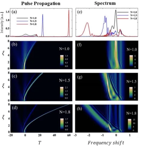
In Chapter 4, we investigate the evolution of optical Airy beams and pulses under various scenarios of nonlinear propagation regimes. Spatial Airy beams are studied in photorefractive media in the presence of either a self-focusing or a self-defocusing nonlinearity, while temporal Airy pulses dynamics are considered in optical fiber propagation under the combined influence of a normal (and an anomalous) group velocity dispersion with a nonlinear Kerr effect. We demonstrate, both numerically and experimentally, a scheme to preserve and control the bending propagation and the spectral features of these optical wave packets even under nonlinear conditions. In particular, we experimentally observe that the linear spectrum of an Airy wave packet is dramatically reshaped under nonlinear propagation, and that most of the spectral content becomes concentrated into self-shifting positive or negative defect, formed by one or two peaks. In correspondence of the defect area, we show that the central frequency of both positive and negative defects linearly changes at each propagation distance, thus indicating a mapping between propagation distance and frequency domain.

(18)

1

Chapter 1

Review of the literature

Self-accelerating beams are optical light localizations that are capable of propagating along curved paths. The Airy beam was the first self-accelerating beam to be introduced and demonstrated in optics. This optical beam can propagate along a parabolic trajectory without experiencing diffraction. Over the last few years, the research on this field has been growing rapidly: New types of self-accelerating beams have been introduced and several applications have been proposed in optics and related fields of physics. In this chapter, we provide a brief overview of the state of the art regarding this subject. Since it expands well beyond the scope of the work reported in this thesis, this literature review does not mean to be exhaustive, but rather introduces the concepts required for understanding what is reported in the next chapters as well as to provide a broader context to the problematics treated in this thesis.

1.1 Diffractive and non-diffractive beams

When a typical laser beam propagates in free-space, its transversal Gaussian intensity profile undergoes a continuous broadening because of diffraction. In the temporal domain, dispersion affects the propagation of an optical Gaussian pulse in a dielectric medium, usually leading to the spreading of the pulse profile and to an increase of its duration. Over the years, non-diffractive and non-dispersive wave packet configurations have been reported in optics as well as in other physical systems. Such optical localized wave packets are shape-preserving during propagation, and can be introduced in the two-dimensional (2D) or three-dimensional (3D) regime. The most widely known non-diffracting wave packet is the Bessel beam which was first introduced by J. Durnin et al. [3-4]. This pioneering work has paved the way to the discovery of other non-diffractive solutions [5-8] including Mathieu [8] and parabolic beams

(19)

2

[6], as well as high-order Mathieu [7] and Bessel beams [5]. In optical systems, such as photonics crystals, exhibiting normal and anomalous diffractions along the two different directions, non-diffractive X-waves [9] and Bessel-like beams [10] have been also introduced. However, such non-diffractive beams exhibit non-diffractive propagation because they convey infinite power. Although not realistic from an experimental viewpoint, in practice, quasi “diffraction-free” beams can be obtained with a finite-energy version – essentially truncated by an aperture. In this case, the diffraction rate can be significantly slowed-down depending on the truncation factor used. Recently, self-accelerating wave packets capable of propagating along a curved trajectory have attracted a great deal of interest. Among them, the Airy beam (or pulse), first introduced in optics, propagates along a parabolic trajectory without any diffraction (or dispersion) [11,13]. Unlike other non-diffractive configurations, Airy wave packets can also exist in the 1D regime. Since its first demonstration, an ever increasing interest has been devoted not only to the study of Airy beams, but also of self-accelerating wave packets in general. In the following chapter, we provide an overview of the recent developments in this research area, essential to placing the results provided throughout this thesis in an appropriate multidisciplinary context, while offering the key scientific concept needed for its understanding. In particular, starting from the concept of Airy beams, we discuss a selection of publications reporting on numerical and experimental studies in the field of self-accelerating wave packets in different frameworks, such as spatial and temporal, linear and nonlinear regime, as well as the most relevant proposed and demonstrated applications.

1.2 Paraxial approximation of the light

In optics, the light propagation is generally described by the Maxwell's equations [1]. Let us consider a scenario where a one-dimensional (1D) optical beam (with x-axis variation) is propagating in free-space along the z-axis, and is also linearly polarized along the x-axis. In this case, the optical beam is only experiencing diffraction along the x-axis. Under this condition, the propagation dynamics of a linearly-polarized electric field

( , , )x z t E x z tx( , , )

(20)

3 2 2 2 2 0 2 2 2 2 0. x x x E E n E z x c t  _ _  _    (1.1)

In the Eq. (1.1), E x z t_x( , , ) the x-component of the electric field, t is the time coordinate. Solutions to Eq. (1.1) can be found by defining E x z tx( , , ) as:

 0

( , , ) ( , ) i kz t ,

x

E x z t E x z e  (1.2)

where E x z( , ) and k = n₀ω₀/c refer to the complex envelope and the wavenumber, respectively, while ω₀ is the angular frequency, n0 is the refractive index, and c the light

velocity. By substituting the latter expression into Eq. (1.1), the complex envelopeE x z( , )of the x-component of the electric field obeys to the Helmholtz equation, explicitly expressed as:

2 2 2 2 2ik 0, z z E E E x      _    (1.3)

Under the paraxial condition, the approximation |2E/z2|2 |k E/ is valid, hence z| propagation dynamics can be described by the paraxial wave equation of diffraction so that:

2 2 1 . 2 0 E E k i z x   _    (1.4)

1.3 Optical Airy beam

In the context of quantum mechanics, M. Berry and N. Balazas theoretically demonstrated in 1979 that the Schrödinger equation describing the propagation of a free particle admits an Airy wave packet as a unique non-spreading solution in the (1+1)D regime [11]. In this paper, not only they demonstrated that an Airy wave packet remains invariant in time, but also that the Airy solution is able to accelerate along a parabolic trajectory in the absence of any external potential. Nevertheless, this work has been set aside for about thirty years due to the fact that such an Airy wave packet could not be experimentally realized in quantum mechanics. Meanwhile, optics has offered, over the years, a fertile and straightforward ground to investigate and demonstrate the proprieties of non-spreading or non-dispersive wave

(21)

4

configurations, even though initially introduced in other physical settings such as atom physics. This analogy origins from the mathematical correspondence between the paraxial Helmholtz equation in optics and the Schrödinger equation in quantum mechanics [48]. In 2007, G. Siviloglou et al. [13-14] proposed and demonstrated experimentally the first generation of an optical Airy wave packet in optics (commonly referred as Airy beam). In what follows, and in in order to introduce the reader to the context, we will provide a detailed digression about their work.

1.3.a Infinite-energy Airy beam

The analysis starts from the normalized (1+1) D paraxial Helmholtz equation that governs the propagation dynamics of the electric field envelope φ( s, ξ ) = E( s, ξ ) of an optical beam:

2 2 1 0, 2 i s





      (1.5)

where s = x /x0 and ξ = z / k0n0 x02denote normalized transverse and longitudinal coordinates, k0 is the vacuum wave number, and x0 is an arbitrary length scale. This equation assumes that

the angle between the propagation axis and wave vectors is small enough so that the wave does not significantly deviate from it. The solution to Eq. (1.5) is a non-spreading Airy beam [11,13]:



,



2 exp exp 3 , 4 2 12 s Ai s  is i    _  _ _ _ _ _       (1.6)

where Ai is the Airy function [12] and φ( s, 0) = Ai(s) is electric field envelope at the input (ξ = 0). Eq. (1.6) shows that this Airy solution is diffraction-free, and experiences a transverse shift along a parabolic curve (s = ξ2/4) during propagation [Fig. 1.1]. An ideal Airy beam is characterized by an asymmetric amplitude profile, formed by a more intense main lobe and an oscillating tail of sub-lobes decaying very slowly for negative values of s, (i.e.

1/2 1/4 3/2

( ) sin(2 / 3 / 4)

(22)

5

Figure 1.1: Propagation dynamics of an inifnite-energy Airy beam. False color plot of the spatial evolution of the Airy beam intensity. The red inset shows the corresponding input intensity profile. (Figure reproduced from Ref. [14]).

For positive values of s, the Airy solution decays exponentially. An interpretation of the acceleration process was provided by D. Greenberger through the principle of equivalence [49]. Other physical interpretations explain the origin of the bending propagation as an interference of straight line rays converging into a caustic [17-18,50-52]. The free-diffraction property is essentially associated with the inherent infinite-energy nature of the beam profile. In fact, an Airy beam is not square integrable



 Ai s( )2ds



  



, and as consequence the

center of mass cannot be defined. This means that the self-accelerating behavior does not violate the Ehrenfest’s theorem [48], describing the motion of a center of mass. In practice, “ideal” Airy beams are impossible to realize experimentally, as they would require an infinite amount of energy. An Airy beam can still be synthesized by using a truncation aperture function, thus obtaining a finite-energy Airy beam (also commonly called Airy beam by extension) [13-14,53].

1.3.b Finite-energy Airy beam

The most common way to obtain a finite-energy Airy beam is by applying an exponential aperture function at the system’s input such as [13-14]:

 

s, 0 ( )expAi s

 

s ,

(23)

6

Where α > 0 is the truncation factor [Fig. 1.2(a)]. The solution to Eq. (1.5) with the initial condition of Eq. (1.7) is found to be:





2 2 3 2 , exp exp , 4 2 12 2 2 s Ai s  i s  i i  is    _   _ _  _ _    _       (1.8)

which reduces to the ideal case when α = 0. Unlike the ideal case, the total power associated to this truncated Airy beam possesses a finite value that is dependent on the truncation parameter

α as: 3 2 1 2 ( ) exp( ) exp 8 3 Ai s s ds        _ _  



(1.9)

Despite the initial truncation, this finite-energy Airy beam still exhibits the property of an ideal Airy beam. It tends to self-accelerate along the same parabolic trajectory with a quasi-diffraction free propagation. In the work proposed by G. Siviloglou et al. [13-14], an Airy beam was propagated up to a distance of 1.25 m, using α = 0.1, x0 = 100 μm and λ = λ0/n0 =

0.5 μm. For these values, the intensity full-wave half maximum (FWHM) width of the (more intense) main lobe is 173 μm.

As shown in Figs. 1.2(b, c), such an Airy beam not only shifts transversally during propagation, but its main hump also remains almost invariant for 75 cm of propagation before being affected by diffraction. Interestingly, the authors also reported that a conventional Gaussian beam with the same initial width would, for the same propagation distance, have undergone a spatial expansion 6 times larger. Moreover, it is possible to define the center of mass of a finite-energy Airy beam. In particular, such a center of mass is constant with distance and is described by the following equation: s( ) 1/N s ( , )s 2ds









3

(24)

7

Figure 1.2: Propagation dynamics of a finite-energy Airy beam. (a) Input intensity profile as a function of the normalized trasversal coordinates s. (b) Intensity distribution showing the propagation dynamincs of a finite-energy Airy beam. (c) Intensity profiles as a function of the real trasversal coordinate x at selected distances z ((i) z = 0 cm, (ii) 31.4 cm, (iii) 62.8 cm, (iv) 94.3 cm, and (v) 125.7 cm). (Figure adapted from Ref. [13]).

The results obtained for the one-dimensional (1D) Airy beams were readily generalized to the (2+1)D scenario. In this case, the solution is found by solving the normalized (2+1)D paraxial equation: 2 2 2 2 ˆ 1 ˆ 1 ˆ 0 2 _x 2 _y i s s      _  _  _    (1.10)

where ˆ



s s_x, _y, is the electric field envelope, s



_x= x / w₀and s_y= y / w₀are, respectively, the normalized transverse coordinates (with w0 scale factor) along the x and y directions, and ξ = z / k0n0 w02 denotes the normalized longitudinal coordinate. αx and αy are the truncation parameters along x and y. One easy way to find a two-dimensional (2D) Airy beam is obtained by multiplying two 1D Airy solutions, respectively along the x and y directions as:



, , 0



 

exp





exp





, ˆ s s_x _y Ai s_x Ai s_y _{x x}s _ys_y

  (1.11)

The evolution of a 2D Airy beam is found as:



, ,





,





,



, ˆ s s_x _y  s_x   s_y 

(25)

8

where 



s_i,



(i = x or y) are the 1D electric field profiles in Eq. (1.8). This 2D Airy beam has an asymmetric intensity profile composed by a highly-confined main lobe spot in the (x- y) plane, and two long tails of sub-lobes [Fig. 1.3(a)]. In the same study, Siviloglou et al. [2-3] also investigated numerically the evolutions of this 2D field configuration by using α_x= α_y = 0.11 and w0 = 53 μm. In contrast to its counterpart in the 1D regime, results

showed quasi non-diffractive propagation. The size of the main lobe spot remained almost invariant up to a distance of 25 cm, while accelerating in the longitudinal direction on the 2D parabolic trajectory with s_x = s_y= ξ2/4. In the transverse plane, such acceleration corresponds to a shift of the 2D Airy intensity pattern along the 45o radial directions, as shown in Fig. 1.3(a, b).

Figure 1.3: Propagation dynamics of a 2D finite-energy Airy beam. (a) Transverse intensity distributions of a 2D finite-energy Airy beam, (a) at the onset of the propagation (z = 0 cm) and (b) after propagation ( z = 50 cm). (Figure adapted from Ref. [13]).

In addition to this analytical and numerical study, the same authors experimentally demonstrated the first generation of optical Airy beams by using a Fourier transform approach [56], as illustrated in Fig. 1.4(a). Their method was based on the properties of the Fourier spatial spectrum of an initial Airy beam in Eq. (1.7), given by:

 

2



3 2 3



, 0 exp exp 3 . 3 i k



k  k



k i



   _  _    (1.13)

(b)

(a)

(26)

9

Such spectrum possesses a Gaussian amplitude, and involves a cubic spectral phase. As a result, an Airy beam can be easily generated by phase-modulating an incident Gaussian beam with a cubic phase distribution in the Fourier domain [Fig. 1.4(b)], and then computing its inverse Fourier transform. The same principle can be readily generalized even for 2D Airy beams. Indeed, the spectrum associated to the envelope field of Eq. (1.11) is













ˆ _, _{, 0} _{, 0} _{, 0}

x y x y

k k k k

    .

Figure 1.4: Experimental demonstration of 1D (and 2D) Airy beams. (a) Scheme of the experimental setup. (Figure adapted from the Ref. [54]). (b-c) Cubic phase masks imprinted onto the incident Gaussian beam to generate (b) a 1D and (c) a 2D Airy beam. (Figures adapted from Ref. [14]). The phase structures shown are “wrapped” between 0 and 2π (i.e. modulo 2π), as typically uploaded in the SLM. The boundary values 0 and 2π correspond, respectively, to the white and black color in the grey scale pattern.

Therefore, a 2D Airy beam can also be easily generated by phase-modulating a circular Gaussian beam with a 2D cubic phase distribution in the in the Fourier domain [Fig. 1.4(c)].

In the setup shown in Fig. 1.4(a), a linearly-polarized Argon-ion Gaussian laser (λ₀= 0.4.88 μm) was firstly collimated to a FWHM of 6.7 mm and then sent to a spatial light

modulator (SLM). Such a computer-controlled liquid crystal device was used to impress the 1D (or 2D) cubic phase modulation onto the incident beam. To generate 1D (or 2D) Airy

(27)

10

beams, a converging cylinder (or spherical) lens (f = 1.2 m) was placed in front of the SLM in order to compute the Fourier transform of the spectrally phase-modulated Gaussian beam. The propagation of the Airy beam was monitored by imaging its intensity pattern using a CCD camera after the back focal plane of the Fourier-transforming lens.

1.4 “Self-healing” of an Airy beam

Along with the convex trajectory and a diffraction-free propagation, another remarkable characteristic of an Airy beam is its “self-healing” property. This feature refers to the ability of an Airy beam of self-reconstructing its shape during propagation, and is of particular importance when it propagates into inhomogeneous media or adverse environments. An inenergy Airy beam is able to self-heal at any propagation distance, while a finite-energy Airy beam manifests self-healing only in the range of distances where a quasi-diffraction free propagation is maintained (as mentioned above). J. Broky et al. studied the self-healing property of optical Airy beam [15]. They carried out a sequence of experimental observations where different parts of a 2D Airy beam were blocked. They observed that the 2D Airy beam could regenerate itself after being blocked by an opaque obstacle, as shown in Figs. 1.5(a, b). Depending on the severity of the perturbation, the distance of self-healing varied during the experiment. In another set of measurements, the authors also demonstrated that an Airy beam can maintain its shape in scattering environments as well as turbulent media, while a standard Gaussian beam was seriously deformed.

The self-healing property is not only a prerogative of Airy beams, but is a characteristic inherent to any non-diffractive beam. An explanation can be obtained using the Babinet’s principle [57]. Indeed, if a non-diffractive beam 𝜑̂(x, y, z = 0) is blocked at the onset of the propagation (z = 0) by a finite energy perturbation ε(x, y, z = 0), the resulting field is expressed as: U(x, y, 0) ≅ 𝜑̂(x, y, 0) ‒ ε(x, y, 0). Due its finite energy nature, the perturbation will diffract out during the propagation. As consequence, at very large distance only the non-diffractive beam will be present, i.e. U x y z( , ,   )2 ˆ( , ,x y z )2.

For an Airy beam, such self-healing process can be understood by studying the internal transverse power flow P_ in the (s_x- s_y) plane. H. Sztul and R. Alfano investigated the

(28)

11

Pointing vector

P

and the angular moment of an unperturbed 2D Airy beam [58], reporting that

P

follows the tangential direction to the curved trajectory. At each propagation distance, the transverse component of the main lobe energy flow ( P_) is thus directed along the 45o radial direction. Correspondingly, the direction of P_ for the beam tails is initially oriented along the negative s_x and s_yaxes, and then tends to rotate towards a direction orthogonal to these axes during propagation. However, the net energy flow remains constant and oriented along the 45o radial direction.

Figure 1.5: Self-healing demonstration of Airy beams. Experimental intensity distributions of a 2D Airy beam (a) at the input (z = 0) where its main lobe is blocked, and (b) after propagation at z = 30 cm. (c) Self-healing mechanism revealed by the transversal power flow P(white arrows), for a 2D Airy beam in which the internal sub-lobes are obstructed at the input distance z = 0. (Figures adapted from Ref. [15]).

Consequently to a perturbation, J. Broky [15] showed how the mechanism of self-healing occurs for an Airy beam. The power flows from the sub-lobes towards the region where the Airy beam has been perturbed by the obstacle. However, the Pointing vector of the main lobe is not involved in the self-healing process. The power flow associated to the main lobe is directed along the

45

oradial direction for sustaining the self-accelerating property, as shown Fig. 1.5(c).

(29)

12

1.5 Paraxial self-accelerating beams

Most of initial progress on the field of self-accelerating beams was limited to the case of parabolic trajectories. In this framework, M. Bandres [45,59] demonstrated that the only orthogonal and complete families of explicit accelerating and diffraction-free solutions of the 2D paraxial wave equation are the infinite-energy Airy and parabolic beams [45]. This means that if the light beam is constrained to remain diffraction-free, the unique valid bending propagation is in fact along a parabolic path. For finite-energy self-accelerating beams, this constraint does not apply. Indeed, E. Greenfield et al. [52] provided the first theoretical and experimental demonstration of quasi-free diffractive 1D self-accelerating beams along arbitrary convex trajectories. Using a caustic theory approach, they engineered the phase structures applied to an incident plane wave (in the real space) towards generating self-accelerating beams with arbitrary convex paths (x = f (z )). To illustrate their theory, several cases of convex trajectories have been considered such as light beams propagating along the curves x = zn (with n = 1.5, 2, 3, 4, 5) or along an exponential trajectory_x _{b e} dz1



 _ (with b and d positive constants) [see e.g. Fig. 1.6(a1, a2), respectively]. The authors showed that the transverse intensity profiles of all these beams exhibit an Airy-like shape and remain non-spreading up to several Rayleigh lengths (z_d= π x02/ k). To experimentally demonstrate their method, a setup very similar to the one described above for the Airy beams has been employed besides the suppression of the Fourier transform lens, due to the imprinting of the desired phase mask directly in the real space [Fig. 1.6(a3)]. Using this framework, we have demonstrated theoretically and experimentally the “Fourier-generation” of 1D (and 2D) self-accelerating beams along arbitrary convex trajectory, for which the caustic theory has been here applied to the Fourier domain (Y. Hu et al. [18]). Such a method permits the design of

spectral phase modulations which can be applied to an incident plane wave in order to

generate any desired convex beam path. Interesting, this approach is not only valid for self-accelerating beams with one single convex trajectory, but can also be generalized to multi-path self-accelerating beams exhibiting more than one light localization [Fig. 1.6(b1)]. Furthermore, by combining these estimated phase structures with appropriate amplitude modulations in the Fourier domain, it becomes possible to generate periodic self-accelerating

(30)

13

beams, i.e. curved beams in which the main lobe evolves along periodical (or zigzag) paths [60], as illustrated in Fig. 1.6(b2). Note that part of these results (Ref. [18]) were actually obtained within the framework of this thesis, and will be further detailed in Chapter 2.

Figure 1.6: Examples of paraxial self-accelerating beams generation. (a1-a3) show the measured intensity distributions of 1D self-accelerating beams propagating along (a1) a cubic polynomial and (a2) an exponential trajectory, obtained by designing the phase modulation in the real space. (a3) shows the schematic experimental apparatus, while the solid green lines in (a1-a2) are analytical predictions. (Figures adapted from Ref. [52]). (b1-b2) show the experimental intensity patterns of (b1) a multi-path (composed by three trajectories) and (b2) a periodic self-accelerating beam, generated by engineering the phase modulation in the Fourier space. (Figures adapted from Refs. [18,60]). (c1-c3) show the experimental generation of non-convex self-accelerating beams. (c1) Experimental intensity distribution for a 1D sinusoidal beam propagating in free space. (c2) Fabricated samples for generating the 1D, 2D sinusoidal beams and circular helical beams. (c3) Experimental setup highlighting the use of the fabricated sample to imprint the desired phase modulation in the Fourier space. (Figures adapted from Ref. [61]).

Recently, Y. Wen et al. [61] developed a method based on a superposition of light caustics which enables the construction of self-accelerating beams whose main lobe follows a non-convex trajectory. In this work, the phase structure for 1D sinusoidal beams [Fig. 1.6(c1)] has

(31)

14

been designed by dividing the entire trajectory in several segments. In each of these segments, the corresponding light localization is a convex path for which both associated spectral amplitude and phase structures are calculated. The entire sinusoidal trajectory was thus obtained by constructing the appropriate spectral amplitude and phase structures through a linear superposition of the initial spatial spectra corresponding to each convex sub-paths. In addition, the authors also demonstrated the generation of 2D sinusoidal and elliptic helical beams, by superimposing two 1D sinusoidal beams (one in the (x,z) plane and the other on the in the (y,z) plane) and controlling their respective phase shifts. An experimental implementation of these non-convex self-accelerating beams has also been performed. The experimental technique is similar as those implemented for typical Airy beams generation, but using, instead of an SLM, several micro-optical structures on quartz glass [Fig. 1.6(c2)] to perform the phase and amplitude modulation onto the incident light in the Fourier domain [Fig. 1.6 (c3)].

1.6 Control of self-accelerating beams

One of most useful feature of self-accelerating beams is the possibility to easily control their curved motion, as well as its transversal profile. As initially investigated by G. Siviloglou et

al. [54], it has been showed experimentally and theoretically that an Airy beam can propagate

along ballistic dynamics by introducing the input condition:

 

s, 0 ( )expAi s

   

s exp ivs ,

   (1.14)

where v is the initial launch angle. The solution to Eq. (1.5) with the initial condition of Eq. (1.14) is found to be [54]:

 





2 2 3 2 2 2 , exp 4 2 exp . 12 2 2 s Ai s i v s v i s v vs v            _        _    _ _   _                     (1.15)

(32)

15

Figure 1.7: Ballistic control of Airy beams. (a1-a3) illustrate infinite-energy Airy beams (α = 0) with initial launch angles (a) v  2, (b) v 0 and (c) v 2. (Figures adapted from Ref. [54]). (b1-b2) illustrate the control of a 2D Airy beam enabled by shifting the relative position of the incident Gaussian beam and cubic phase mask in the Fourier space. (Figures adapted from Ref. [62]). (b1) shows the schematic experimental setup and (b2) shows several snapshots of the measured transverse intensity patterns at selected distances (z = 0, 15 and 30 cm), for two different propagation dynamics. Upper snapshots in (b2) correspond to a perfect axial alignment between the Gaussian beam and the cubic phase mask. Middle snapshots in (b2) highlight the ballistic dynamics of the 2D Airy beam when the cubic phase mask is shifted downward along the vertical direction ky. Lower snapshots in (b2)

highlights the dynamics of the 2D Airy beam when both the cubic phase mask and the Gaussian beam are oppositely shifted along the vertical direction ky.

When v is positive (negative), the Airy beam is launched upwards (downwards) [Figs. 1.7(a2-a3)]. Airy beams with different angles can be launched by transversally shifting up or down the Fourier-transforming cylindrical lens [56], indicated with L in the setup shown in Fig. 1.4.

(33)

16

It is worth mentioning that, when the Airy beam moves along a ballistic path, the center of gravity evolves along the line given by: 3

( ) (4 1) / 4

s  v    .

In a related work, Y. Hu et al. [62] demonstrated another way to control the motion of 2D Airy beams. The authors showed that, when both the cubic phase mask and incident Gaussian beam centers are overlapped on the z-axis, the 2D Airy beam propagates along a parabolic trajectory and the peak intensity is located at the onset distance [z = 0 cm in Figs. 1.7(b1, b2) (upper panel)]. By vertically shifting the cubic phase mask with respect to the z-axis, as shown in Fig. 1.7(b1), the 2D Airy beam evolves along a ballistic trajectory. In this case, the peak intensity is reached in correspondence of the maximum height [Fig. 1.7(b2) (middle panel)]. Additionally if the Gaussian beam is also shifted vertically at the opposite location of the cubic phase mask, the peak intensity of the 2D Airy beam appears at the end of the trajectory [z = 30 cm in Fig. 1.7(b2) (lower panel)]. In this way, the position of the peak intensity can be also controlled along the propagation distance. Moreover, the horizontal displacement of either the cubic phase mask or the Gaussian beam leads to a projectile motion which can be set into any arbitrary direction. In this case, the intensity profile of the 2D Airy beam shows asymmetric wings.

Figure 1.8: Deformed 2D Airy beams. Intensity distributions corresponding to a deformed Airy beam with (a) a right, (b) an acute and (c) an obtuse angle between the two wings. (Figure adapted from Ref. [63]).

(34)

17

Another way to control the parabolic trajectory of a 2D Airy beam is by deforming the two long sub-lobe tails [63]. In particular, the electric field envelope of a deformed Airy beam is expressed by:



, , 0



 

( )

 

( )

ˆ S_x S_y Ai S_x expS_x Ai S_y expS_y

  (1.16)

where S_x  (rs_xs_y/ ) / 2r and S_y (rs_xs_y/ ) / 2r , and r is the parameter determining the degree of deformation of the Airy beam. A “classic” 2D Airy beam whose tails form a 90o

angle corresponds to r = 1 [Fig. 1.18(a)]. Otherwise, the angle between the Airy beam tails changes, as shown in Figs. 1.18(b-c). In particular, if r > 1 (r < 1) this angle is acute (obtuse), and the correspondingly deformed Airy beam experiences a decreased (increased) acceleration. Additionally, a slightly-deformed Airy beam tends to restore the standard angle (90o degree) during propagation. However, large deviations lead to beam propagations where an initial obtuse angle evolves towards an acute one, and vice versa.

Figure 1.9: Experimentally obtained quasi-Airy beams corresponding to different disturbance factors θ₁ and θ₂. (a1-d1) illustrate the wrapped spectral phase masks obtained by setting the disturbance factors respectively to (a1) θ₁ / 6 and θ₂  / 3, (b1) θ₁3 / 4 and θ₂0, (c1)

0

1

θ  and θ₂/ 2,(d1) θ₁7 / 6 and θ₂  / 4. (a2-d2) are the corresponding transverse intensity distributions of the generated quasi-Airy beams. (Figure adapted from Ref. [64]).

(35)

18

In a similar work, Y. Qian and S. Zhang [64] deformed the spectral cubic phase mask by means of the two disturbance factors ₁and ₂(varying in the range between 0 and 2π), as:





















2 3 2 1 1 2 2 3 1 1 2 2 / 3 3 . ˆ _, _{, 0} / x y x y x y x y x y

exp cos k sin sin k

k k k k cos

exp i k cos k sin i k sin k cos

              _ _         _    _   (1.17)

In this way, they introduced a new family of 2D Airy beams (called quasi-Airy beams), of which some examples are shown in Figs. 1.9(a1-d2). By adjusting the angle between the wings, such quasi-Airy beams can propagate along designed trajectories. The Airy beam can be regarded as special case of a quasi-Airy beam whose wings are reciprocally orthogonal. During propagation, a quasi-Airy beams generates two separate parabolic trajectories, one for the main lobe and the other one carrying the peak intensity. The two parabolic trajectories overlap when the angle between the wings is 90o degree (2D Airy beam) - see Ref. [64] for more details.

However in all these previously mentioned cases, the control of Airy beams is achieved in free-space. It is worth mentioning briefly that other ways to manipulate the Airy beam dynamics exist by means of external potentials, such as linear [29,65-66] and harmonic [67-68] potentials. For example, an optically-induced refractive index gradient along the x-axis can modulate the bending propagation of 1D (or 2D) Airy beams, thus leading to beam dynamics where the parabolic acceleration is increased, reduced or even suppressed [29]. A linear potential can also be used to shape the propagation trajectory of an Airy beam. N. Efremidis [65] engineered the beam trajectory of 1D (and 2D) Airy beams by designing transversely linear potentials with longitudinal (z-axis) index gradients and finding the associated initial input conditions (i.e. spatial displacement and tilt). As an illustrative example, the author estimated the potential gradients and the initial parameters for an Airy beam to propagate along a polynomial law, sinusoidal, logarithmic and hyperbolic trajectory, as well as a 2D Airy beam to follow a spiral trajectory in space. Finally, under an external harmonic potential [67], the Airy beam follows an unusual oscillating propagation.

(36)

19

1.7 Non-paraxial self-accelerating beams

The self-accelerating beams described until now are solutions of the (1+1)D (or (2+1)D)

paraxial Helmholtz equation of diffraction, whose normalized form is Eq. (1.5) (or correspondingly Eq. (1.10)). Nevertheless, this paraxial wave equation only represents an

approximation to the Helmholtz equation, describing the actual propagation of linearly-polarized monochromatic optical beams. In the (2+1)D regime, this equation reads:

2 2 2 2 2 2 2 ˆ ˆ ˆ ˆ 0 k z x y



_

 _ _ _ _    (1.18)

Where 𝜑̂(x, y, z) is the electric field envelope, x and y denote the transverse coordinates, and z is the longitudinal coordinate. Here, k = k₀n₀indicates the wavenumber, where k₀is the vacuum wavenumber and n₀is the refractive index. Solutions to Eq. (1.18) can be found in the Fourier regime, as:

  2 2 2 2 1 _ˆ ˆ( , , ) ( , , 0) . 4 x y x y iz k k k i k x k y x y x y x y z k k e e dk dk          



(1.19) where ˆ( , , 0) ˆ( , , 0) i k x k y x y  x y k k  x y e  dxdy 

 

_

is the input spectrum. In Eq. (1.19), the

positive sign of the first exponential term accounts for forward propagations, while a negative sign refers to backward propagations. Looking at the Fourier regime, the spatial frequencies in charge of the propagation are in the range k2kx2ky2  , while those out of this range are 0 associated to the generation of evanescent waves. To obtain the paraxial wave equation from Eq. (1.19), the condition of a slowly-varying envelope must be satisfied, i.e.

2 2

|ˆ/z | 2k|ˆ/ . In the Fourier regime, such condition means to consider optical z| beams whose spatial spectrum is confined in a small range of spatial frequencies so that k >> k_x and k >> k_y. From a physical viewpoint, the paraxial wave equation can thus only describe the propagation of self-accelerating beams when the trajectory is limited to small angles. For larger angles, such beams are not anymore shape-preserving. For instance, in the paraxial regime, an ideal Airy beam preserves its amplitude for all distances. When propagating under non-paraxial condition, its trajectory tends to break after short propagation

(37)

20

distances (or small angles), thus becoming no longer shape-preserving [69] [see Fig. 1.10(g)]. This constitutes a serious limitation as the propagation angle of a self-accelerating beam continuously increases, and after a given distance, the beam dynamics actually fall into the non-paraxial regime. Indeed, steeper angles involve more spatial frequencies to sustain the beam acceleration. Therefore, it is important to find self-accelerating beams capable of maintaining the bending propagation, even in the non-paraxial regime. Further research on this field has been undertaken to solve this problem. In the last five years, several non-diffractive self-accelerating beam solutions to the Helmholtz equation have been introduced and demonstrated [Fig. 1.10].

Figure 1.10: Non-paraxial self-accelerating beams obtained by solving the Helmholtz equation in different conical coordinate systems. (a) Schematic of different trajectories related to a Mathieu non-paraxial accelerating beam (NAB) for various ellipse parameters (i.e. semi-axes a and b) The case a = b corresponds to a Bessel NAB. (b) Amplitude of NABs at z = 0 for a < b (red solid line), a = b (black dotted line) and a > b (blue dashed line). Propagation dynamics of the Mathieu NABs for (c) a < b, (d) a = b and (e) a > b. (f-g) Comparison between the propagation dynamics of (f) a Weber NAB and an (g) Airy beam. (h) Amplitude of Weber NAB (solid blue line) and Airy beam (red dotted line) at z = 0. The white dashed line in (c-g) marks the input distance z = 0. (Figure adapted from Ref. [21]).