Constraint modelling and solving of some verification problems

(1)

HAL Id: tel-01743851

https://tel.archives-ouvertes.fr/tel-01743851

Submitted on 26 Mar 2018

HAL is a multi-disciplinary open access

archive for the deposit and dissemination of sci-entific research documents, whether they are pub-lished or not. The documents may come from teaching and research institutions in France or abroad, or from public or private research centers.

L’archive ouverte pluridisciplinaire HAL, est destinée au dépôt et à la diffusion de documents scientifiques de niveau recherche, publiés ou non, émanant des établissements d’enseignement et de recherche français ou étrangers, des laboratoires publics ou privés.

Constraint modelling and solving of some verification

problems

Anicet Bart

To cite this version:

Anicet Bart. Constraint modelling and solving of some verification problems. Programming Languages [cs.PL]. Ecole nationale supérieure Mines-Télécom Atlantique, 2017. English. �NNT : 2017IMTA0031�. �tel-01743851�

(2)

Thèse de Doctorat

Anicet BART

Mémoire présenté en vue de l’obtention du

grade de Docteur de l’École nationale supérieure Mines-Télécom Atlantique Bretagne-Pays de la Loire

sous le sceau de l’Université Bretagne Loire

École doctorale : Mathématiques et STIC (MathSTIC) Discipline : Informatique, section CNU 27

Unité de recherche : Laboratoire des Sciences du Numérique de Nantes (LS2N) Soutenue le 17 octobre 2017

Thèse n°: 2017IMTA0031

Constraint Modelling and Solving

of some Verification Problems

JURY

Présidente : Mme_{Béatrice BÉRARD, Professeur, Université Pierre et Marie Curie, Paris-VI}

Rapporteurs : M. Salvador ABREU, Professeur, Universidade de Évora, Portugal

Mme_{Béatrice BÉRARD, Professeur, Université Pierre et Marie Curie, Paris-VI}

Examinateurs : M. Nicolas BELDICEANU, Professeur, Institut Mines-Télécom Atlantique, Nantes M. Philippe CODOGNET, Professeur, Université Pierre et Marie Curie, Paris-VI Invité : M. Benoît DELAHAYE, Maître de conférence, Université de Nantes

Directeur de thèse : M. Éric MONFROY, Professeur, Université de Nantes

(3)

(4)

Constraint Modelling and Solving

of some Verification Problems

Mémoire présenté en vue de l’obtention du grade de

Docteur de l’´

Ecole nationale sup´

erieure Mines-T´

el´

ecom

Atlantique Bretagne-Pays de la Loire - IMT Atlantique

sous le sceau de l’Universit´e Bretagne Loire

Anicet BART

´

Ecole doctorale : Sciences et technologies de l’information, et math´ematiques Discipline : Informatique et applications, section CNU 27

Unit´e de recherche : Laboratoire des Sciences du Num´erique de Nantes (LS2N - UMR 6004)

Directeur de thèse : Pr. Éric MONFROY, professeur de l’Université de Nantes

(5)

(6)

v

Jury

Directeur de th`ese :

M. ´Eric MONFROY, Professeur, Universit´e de Nantes Co-encadrante :

Mme Charlotte TRUCHET, Maˆıtre de conf´erence, Universit´e de Nantes Rapporteurs :

M. Salvador ABREU, Professeur, Université d’Évora, Évora (Portugal)

Mme Béatrice BÉRARD, Professeur, Université Pierre et Marie Curie, Paris-VI Examinateurs :

M. Nicolas BELDICEANU, Professeur, Institut Mines-Télécom Atlantique, Nantes M. Philippe CODOGNET, Professeur, Université Pierre et Marie Curie, Paris-VI

Invit´e :

(7)

(8)

vii

Constraint Modelling and Solving

of some Verification Problems

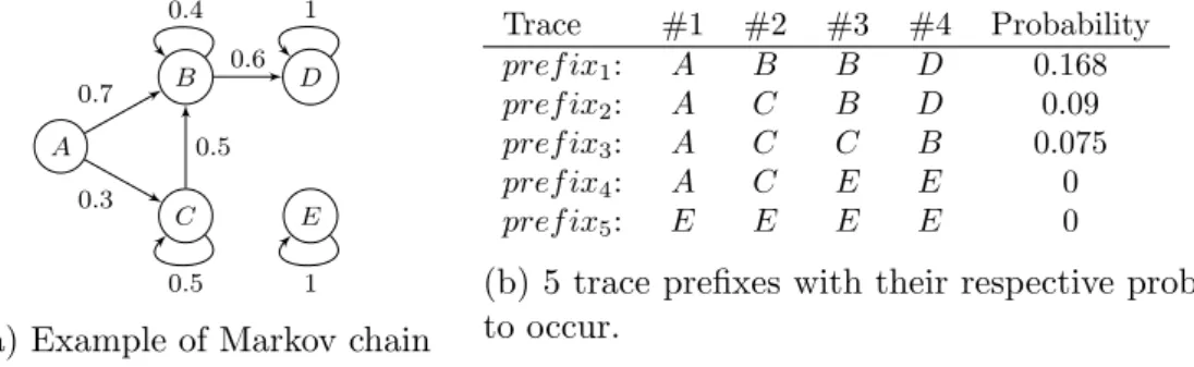
Short abstract: Constraint programming offers efficient languages and tools for solving combinatorial and computationally hard problems such as the ones proposed in program verification. In this thesis, we tackle two families of program verification prob-lems using constraint programming. In both contexts, we first propose a formal eval-uation of our contributions before realizing some experiments. The first contribution is about a synchronous reactive language, represented by a block-diagram algebra. Such pro-grams operate on infinite streams and model real-time processes. We propose a constraint model together with a new global constraint. Our new filtering algorithm is inspired from Abstract Interpretation. It computes over-approximations of the infinite stream values computed by the block-diagrams. We evaluated our verification process on the FAUST language (a language for processing real-time audio streams) and we tested it on exam-ples from the FAUST standard library. The second contribution considers probabilistic processes represented by Parametric Interval Markov Chains, a specification formalism that extends Markov Chains. We propose constraint models for checking qualitative and quantitative reachability properties. Our models for the qualitative case improve the state of the art models, while for the quantitative case our models are the first ones. We imple-mented and evaluated our verification constraint models as mixed integer linear programs and satisfiability modulo theory programs. Experiments have been realized on a PRISM based benchmark.

Keywords: Constraint Modelling - Constraint Solving - Program Verification - Ab-stract Interpretation - Model Checking

(9)

viii

Mod´

elisation et r´

esolution par contraintes

de probl`

emes de v´

erification

Résumé court : La programmation par contraintes offre des langages et des outils permettant de résoudre des problèmes à forte combinatoire et à la complexité élevée tels que ceux qui existent en vérification de programmes. Dans cette thèse nous résolvons deux familles de problèmes de la vérification de programmes. Dans chaque cas de figure nous commen¸cons par une étude formelle du problème avant de proposer des modèles en contraintes puis de réaliser des expérimentations. La première contribution concerne un langage réactif synchrone représentable par une algèbre de diagramme de blocs. Les pro-grammes utilisent des flux infinis et modélisent des systèmes temps réel. Nous proposons un modèle en contraintes muni d’une nouvelle contrainte globale ainsi que ses algorithmes de filtrage inspirés de l’interprétation abstraite. Cette contrainte permet de calculer des sur-approximations des valeurs des flux des diagrammes de blocs. Nous évaluons notre processus de vérification sur le langage FAUST, qui est un langage dédié à la génération de flux audio. La seconde contribution concerne les systèmes probabilistes représentés par des chaˆınes de Markov à intervalles paramétrés, un formalisme de spécification qui étend les chaˆınes de Markov. Nous proposons des modèles en contraintes pour vérifier des pro-priétés qualitatives et quantitatives. Nos modèles dans le cas qualitatif améliorent l’état de l’art tandis que ceux dans le cas quantitatif sont les premiers proposés à ce jour. Nous avons implémenté nos modèles en contraintes en problèmes de programmation linéaire en nombres entiers et en problèmes de satisfaction modulo des théories. Les expériences sont réalisées à partir d’un jeu d’essais de la bibliothèque PRISM.

Mots clés : modélisation par contraintes - résolution par contraintes - vérification de programmes - interprétation abstraite - vérification de modèles

(10)

Contents 1

Chapter

1

Introduction

4 Chapter 1. Introduction Computer scientists started to write programs in order to produce softwares realizing dedicated tasks faster and more efficiently than a human could perform. However, in ad-hoc developments the more complex is the problem to solve the longer it takes to write its corresponding solving program. Moreover, few modifications in the description of the problem to solve may impact many changes in the program. The artificial intelligence research domain tries to develop more generic approaches such that a single artificially intelligent program may solve a wide variety of heterogenous problems. Constraint pro-gramming is a research axis in the artificial intelligence community where constraints are sets of rules to be satisfied and the intelligent program must find a solution according to these rules. Thus, the objective of the constraint programming community is to produce languages and tools for solving constraint based problems. Such problems are expressed in a declarative manner where programs consist in a set of rules (called constraints) to be satisfied. Thus, a constraint programming user enumerates his/her rules and uses a black-box tool (called solver) for solving his/her problem. These are two major research ac-tivities in constraint programming: modelling and solving. The modelling activity works on the expressiveness of the constraint language and manipulates constraint programs in order to improve the resolution process. The solving activity consists in developing algorithms, tools, and solvers for improving the efficiency of the resolution process.

For the last decades computers and information systems have been highly democra-tized for private and company usages. In both contexts, more and more complex systems are developed in order to realize a wide variety of applications (smart applications, embed-ded systems for air planes, medical robot assistants, etc.). As for many other production fields, writing systems must respect quality rules such as conformity, efficiency, and robust-ness. In this thesis, we are concerned by the verification problem consisting in verifying if an application, a program, a system matches its specifications (i.e., its expected behavior). This concern gained an important interest after social or business impacts are identified, or after past failures. One of the most remarkable examples is the crash of the Ariane 5 missile, 36 seconds after its launch on June 4, 1996. The accident was due to a conversion of a 64-bit floating point number into a 16-bit integer value. Another example is the bug in Intel’s Pentium II floating-point division unit in the 90’s, which forced to replace faulty processors, severely damaged Intel’s reputation, and implied a loss of about 475 million US dollars. These events happened in the 90’, and software are now more and more used to automatically control critical systems such as nuclear power plants, chemical plants, traffic control systems, and storm surge barriers. Furthermore, even programs with less critical impact require attention, since the competition between products gives benefits to the systems with less bugs, a better reactivity, etc. Thus, the verification objective is to attest the validity of a system according to an expected behavior.

While such problems may be solved using add-hoc techniques or proper tools, it ap-pears that by nature or by reformulation of the problem, constraint programming offers

(14)

1.1. Scientific Context 5

effective solutions. For instance, the system/program can be formulated as a set of rules and the expected behavior as a set of constraints. Thus, verifying the validity of the system/program behavior consists in determining if satisfying the rules implies to satisfy the expected behavior. On the other hand, some verification considerations may produce combinatorial problems. In this context constraint programming clearly appears as a suitable solution. In this thesis we tackle program verification problems as applications to be treated using constraint programming.

1.1 Scientific Context

As said before this thesis concerns constraint programming modelling and solving for some program verification problems. In this section we briefly present all the scientific context of the thesis by identifying separately the various scientific thematics tackled in this manuscript. We start by presenting constraint modelling and solving. Then, we continue with the two program verification approaches used in this thesis, and we conclude by presenting the two programming paradigms to be verified in this thesis.

Constraint Modelling. A Constraint Satisfaction Program (CSP for short) is a set of constraints over variables each one associated with a domain. Thus, constraint mod-elling consists in formulating a given problem into a CSP. There exist various research communities each one dedicated to model families of CSPs. Recall first that the general problem of satisfying a CSP (i.e., finding a valuation of the variables satisfying all the constraints in the CSP) is a hard problem. There exists CSP families being tractable in exponential, polynomial, or ever linear time. In this thesis we consider constraint mod-elling ranging from mathematical programming such as continuous and mixed integer linear programing (respectively LP and MILP for short), finite and continuous domains programs without linearity restrictions on the constraints (respectively named FD and CD for short), and Satisfiability Modulo Theory (SMT for short) mixing Boolean and theories such as arithmetics. See Section2.2 for more details.

Constraint Solving. Various tools, named solvers, have been developed for solving CSP instances. Each one is mainly specialized to solve specific CSP families (e.g., un-bounded integer linear arithmetics, constraints over variables with finite domain, continu-ous constraints). The combinatorics implied by the relations between the variables in the constraints makes a CSP hard to solve. This requires to explore search spaces composed of all the valuations possibly candidate for solving the problem. However, the size of such search space is exponential in terms of the problem sizes (number of variables) in general. Huge research efforts has been put into solvers in order to propose tools for (intelligently) explore huge search spaces and solve CSP instances. See Section2.3 for more details.

(15)

6 Chapter 1. Introduction Program Verification A program describes the behavior of a possibly infinite process by defining possible transitions from states to states. Due either to the runtime envi-ronment or to the non determinism of the state successions, one program may have a finite or even an infinite number of possible runs. Also, according to the nature of a program its runs may encounter either a finite or an infinite number of states in theory. Thus, program verification consists in determining if the program traces (i.e., the state sequences realized by the runs) respect a given property. These properties may be time dependent (e.g., for each run the state A must be encountered after the state B, the state A must not be encountered before a given time t) or time independent (e.g., for each run all the variables are bounded by given constants). There are two main approaches for verifying properties on program: dynamic analysis vs. static analysis. Dynamic analysis requires to run the program to attest the validity of the property. On the contrary, static analysis performs verification at compilation time without running the program/system (roughly speaking dynamic analysis can be considered as an online process compared to static analysis which is an offline process). See Section 3.1 for more details. In this thesis we only consider complete static analyzes of programs with infinite runs (i.e., we do not consider dynamic and bounded analyzes).

Abstract Interpretation. Abstract Interpretation is a program verification technique for static program analysis. In this context, we consider programs with unbounded run-ning times and infinite state systems. Recall that in such cases the general program verification problem is undecidable since this class of problems contains the halting prob-lem. Thus, Abstract Interpretation provides a verification process, which terminates, using over-approximations of the semantics of the program to verify. Indeed, well chosen abstractions produce semi-decidable problems. Thus, verification tools based on abstract interpretation either prove the validity of the property or may not conclude. Hence, such method cannot find counter-examples and falsify properties. See Section 3.2 for more details.

Model Checking. Model Checking is a program verification technique for static pro-gram analysis. As for Abstract Interpretation, propro-grams/models to be verified may have unbounded running times and infinite state space. Thus, model checking is a verification method that explores all possible system states. In this way, it can be shown that a given system model truly satisfies a certain property. Hence, such method proves the validity or the non validity of the property. More specifically, it can return a counter-example in non validity case. See Section 3.3 for more details.

Synchronous Reactive Language. Motivated by the nature of embedded controllers requiring to be reactive to the environment at real-time, synchronous languages have been designed for programming reactive control systems. These languages naturally deal with

(16)

1.2. Problems and Objectives 7

the complexity of parallel systems. Indeed, parallel computations are realized in a lock-step such that all computations are synchronized reactions. Hence, this synchronization ensures by construction a guarantee of determinism and deadlock freedom. Finally, these languages abstract away all architectural and hardware issues of embedded, distributed systems such that the programmer can only concentrate on the functionalities. Instances of such languages are Faust, Lustre, and Esterel and have been successfully used in the context of critical systems requiring strong verification (e.g., space applications, railway, and avionics) using certified compiler (e.g., Scade [Sca] tool from Esterel Technologies providing a DO-178B level A certified compiler). Chapter 4 concerns the verification of synchronous reactive languages.

Probabilistic Programming Language. Various systems are subject to phenomena of a stochastic nature, such as randomness, message loss, probabilistic behavior. Proba-bilistic programming languages are used to describe such systems using probabilities to define the sequence of states in the program. One of the most popular probabilistic mod-els for representing stochastic behaviors are the discrete-time Markov Chains (MCs for short). Instance of probabilistic programming languages for writing MCs are Problog and Prism. Chapter5 concerns the verification of models extending the Markov chain model describing parametrized probabilistic systems.

1.2 Problems and Objectives

As presented in the previous sections, program verification is a computationally hard problem with major issues. Recall first that a program describes the behavior of a pos-sibly infinite process by defining possible transitions from states to states. However, the verification is performed on an abstraction of the program named model1_{. In this thesis,} we consider finite models with infinite state spaces and infinite runs.

Even if a program admits a priori an infinite state space its executions may encounter a (potentially infinite) subset of the declared state space. Thus, one would like to deter-mine this smaller state space in order to verify the non reachability of undesired states. This problem is reducible to the search of program over-approximations, i.e., bound-ing all the program variables. This is an objective of Abstract Interpretation where the program describing precisely the system evolution from a state to another, named the concrete program, is abstracted. This abstracted construction is related to the concrete program in such a manner that if an over-approximation holds for the abstraction then, this approximation also holds for the concrete program. Furthermore, constraint pro-grams allow to describe over-approximations such as convex polyhedrons using linear

1

We already introduced the word model in the constraint programming context. The reader must be careful that this word has an important role in both contexts.

(17)

8 Chapter 1. Introduction constraints, ellipsoids using quadratic constraints, etc. Thus, since constraint program-ming is a generic declarative prograprogram-ming paradigm it may be seen as a verification process for over-approximating variable in declarative programs. In the first contribution, we con-sider a block-diagram language where executions are infinite streams and the objective is to bound the stream values using constraint programming.

However, bounding the state space is not enough for some verification requirements. In our second problem, the objective is to determine if a specific state is reachable at execution time. Indeed, abstractions can only determine if a specific state is unreachable. For this verification problem, we consider programs representable as finite graph structures where the nodes form the state space and the edges give state to state transitions. Thus, verifying the reachability of a state in such a structure is performed by activating or deactivating transitions in order to reach the target state. However, these activations can be restricted by guards, or other structural dependent rules. Clearly, this corresponds to a combinatoric problem to solve. For this reason, since one of the objectives of constraint programming is to solve highly combinatorial problems, the verification community is interested in the CP tools.

Some links between constraint programming and program verification are presented in Section 3.4. To conclude, constraint programming proposes languages to model and solve problems by focusing on the problem formulation instead of the resolution process. Program verification leads to problems which by definition or by nature are close to constraint programs. Thus, the verification community uses constraint programming tools for developing analyzers instead of producing ad-hoc algorithms. In this thesis, we position ourself as constraint programmers and we consider verification problems as applications. Thus, our objective is to present how the constraint programming advances in modelling and solving helps to answer some verification problems.

1.3 Contributions

The contributions are split into two distinct chapters, and they are related to different verification research axes, but both using constraint programming. The first contribution applies constraint programming to verify some properties of a real-time language, while the second one is about verification of extensions of Markov chains. Here are the abstracts of these two contributions.

Verifying a Synchronous Reactive Language with constraints (Chapter 4). Formal verification of real time programs in which variables can change values at every time step, is difficult due to the analyses of loops with time lags. In our first contribution, we propose a constraint programming model together with a global constraint and a filtering algorithm for computing over-approximation of real-time streams. The global

(18)

1.4. Outline 9

constraint handles the loop analysis by providing an interval over-approximation of the loop invariant. We apply our method to the FAUST language which is a language for processing real-time audio streams. We conclude with experiments that show that our approach provides accurate results in short computing times. This contribution has been published in a national conference [1], an international conference [2], and a journal [3]. Verifying a Parametric Probabilistic Language with constraints (Chapter 5). Parametric Interval Markov Chains (pIMCs) are a specification formalism that extends Markov Chains (MCs) and Interval Markov Chains (IMCs) by taking into account impreci-sion in the transition probability values: transitions in pIMCs are labeled with parametric intervals of probabilities. In this work, we study the difference between pIMCs and other Markov Chain abstractions models and investigate the three usual semantics for IMCs: once-and-for-all, interval-Markov-decision-process, and at-every-step. In particular, we prove that all these semantics agree on the maximal/minimal reachability probabilities of a given IMC. We then investigate solutions to several parameter synthesis problems in the context of pIMCs – consistency, qualitative reachability, and quantitative reachability – that rely on constraint encodings. Finally, we conclude with experiments by implementing our constraint encodings with promising results. This contribution has been published in a national conference [4], an international workshop without proceedings [5], and an international conference [6] (to appear).

1.4 Outline

The thesis in organized in four main chapters. Chapter2presents the constraint program-ming paradigm. Chapter 3 introduces program verification/model checking problems. We conclude this chapter by briefly introducing the two verification methods named Ab-stract Interpretation and Model Checking in order to motivate the two following chapters which respectively use these verification methods. Chapter 4 contains our first contri-bution. This chapter proposes a constraint programming model together with a global constraint and a filtering algorithm inspired from abstract interpretation for computing over-approximation of real-time streams. This chapter is also illustrated and validated by some experiments. Chapter 5 contains our second contribution. This chapter proposes constraint programming models for verifying qualitative and quantitative properties of parametric interval Markov chains with a model checking objective. This chapter also concludes with experiments. Note that both contribution chapters are self-contained including introduction, motivation, background, state of the art, contributions, and bib-liography. Finally, Chapter6 concludes this thesis document.

(19)

(20)

11

Chapter

2

Constraint Programming

2.1 Introduction

Computer scientists started to write programs in order to produce softwares realizing dedicated tasks faster and more efficiently than a human could perform. However, in ad-hoc developments the more complex is the problem to solve the longer it is to write its corresponding solving program. Moreover, few changes in the description of the problem to solve may impact many changes in the program. Thus, the artificial intelligence research domain tries to develop more generic approaches such that a single artificially intelligent program may solve a wide variety of heterogeneous problems. Among all possible artificial intelligences, we focus in this thesis on those dealing with constraint based problems. In such problems, one can enumerate a set of objects with possibly many different states for each object and a set of accepted configurations over these objects w.r.t. the states (cf. Definition 2.1.1).

Definition 2.1.1 (Constraint Based Problem). Let A be a set of objects, and S be a set of object states. A Constraint Based Problem_{P over objects A with states S represents a} set of configurations (i.e., a set of associations between objects from A and states in S). Formally _{P ⌘ L s.t. L ✓ S}A_.

In this chapter, we first present constraint modelling (i.e., variables, domains, straints, and constraint programs definitions) and various research axes dedicated to con-straint modelling (SAT, CP, LP, etc.). Then, we present these research axes dealing with constraint programs by describing their common resolution processes and their specific strategies developed in each one.

Restrictions. In this thesis we consider modelling with real, integer, and Boolean vari-ables with finite or infinite domains without restrictions on the constraints (e.g., enu-merations, linear and non-linear inequations, Boolean compositions, global constraints) using the existential quantification of variables and being time-independent1_{. Finally, we} consider complete methods for solving such models.

2.2 Constraint Modelling

Constraint modelling is the action of formulating a given constraint based problem into a constraint based program. Definition 2.1.1 recalled that a constraint based problem is described by a set of objects, a set of object states, and gathered into a set of con-figurations. Constraint programming uses a dedicated vocabulary. In the following we take care to well separate the constraint based problems from constraint based programs. Indeed constraint based problems are commonly expressed in a natural language while

1

Note that Chapter4models a problem with time-dependency (verification of a reactive synchronous programming language). However the constraint modelling is time-independent.

(22)

2.2. Constraint Modelling 13 5

Z0Z0Z

4

0Z0Z0

3

Z0Z0Z

2

0Z0Z0

1

Z0Z0Z

a b c d e

Q

(a) Empty 5⇥5 chessboard with 5 Queens. 5

Z0ZQZ

4

0L0Z0

3

Z0Z0L

2

0ZQZ0

1

L0Z0Z

a b c d e

.

(b) Queens positioning re-specting ”no threat” rules.

5

Z0Z0L

4

0ZQZ0

3

ZQZ0Z

2

0Z0L0

1

L0Z0Z

a b c d e

.

(c) Queens positioning violating twice the diagonal ”no threat” rule.

Figure 2.1: 5-Queens problem illustrated with: (a) its 5_{⇥5 empty chessboard and its} 5 queens; (b) a queen configuration satisfying the 5-Queens problem; and (c) a queen configuration violating the 5-Queens problem.

constraint programs are expressed in a mathematical (or mathematical-like) language or a programming language. A constraint program uses variables associated with domains linked by constraints. Roughly speaking, the variables with their domains will model the objects with their states in the constraint based program while the constraints will model the configurations in the constraint based program. We now present a wide landscape of variables, domains, and constraints encountered in constraint modelling while encoding a constraint based problem into a constrained program.

Example 1 (n-Queens Problem). The n-Queens problem will be our backbone example for illustrating constraint modelling and solving in this section. Let n be a natural number. Thus we consider an n_{⇥ n chessboard and n queens. The n-Queens Problem objective} is to place the n queens on the chessboard such that no two queens threaten each other (i.e., no two queens share the same row, column, or diagonal). In this example, objects are the n queens and states are the n_{⇥ n cells of the chessboard. Thus, a configuration} is an arrangement of the n queens on the chessboard.

2.2.1 Variables and Domains

A constraint based problem is described by a set of variables, each variable being associ-ated with a non-empty set called its domain. From now on in this section, X will refer to a set of n variables x1, . . . , xn, Dx will be the domain associated to the variable x 2 X, and D will contain all the domains associated to the variables in X. We identify four variable types according to their domain. We say that a variable x with domain Dx is:

• a Boolean variable iff its domain is a binary set (i.e., Dx={true, false}) • an integer variable iff its domain only contains integers (i.e., Dx ✓ Z)

(23)

• a real variable iff its domain only contains real numbers (i.e., Dx ✓ R)

A domain can be given in extension by enumerating all the elements composing it or in intension using an expression representing all its elements. One common compact representation is the interval representation together with the union of intervals. Formally, let E _{✓ R be a non-empty totally ordered set and a, b 2 R}2 _{be two interval endpoints. We} write IE([a, b]) for the set containing all the (closed, semi-opened, opened) intervals subsets of the interval [a, b]_{✓ E. When modelling, we usually separate real variables with interval} domains from others. The first ones are called continuous variables while the remaining are called discrete variables. Furthermore, we separate finite variables (i.e., variables whose domains have a finite number of elements) from infinite variables. For instance a finite variable can be introduced by domain enumeration (e.g., domain _{{1, 2, . . . , 50})} and infinite variables can be defined by interval domain (e.g., domain [_{−1, 1] subset of R).} Note that there exists other domains such that the symbolic domains where each domain may contain an infinite number of possibly ordered symbols, or the set domains where each domain element is a set of values. In this thesis we perform constraint modelling with Boolean, integer, rational, and real-number domains. Finally, a valuation of the variables in X0 _{✓ X is a mapping v associating to each variable in X}0 _{a value in its domain (i.e.,} v : X0 _{! D s.t. v(x) 2 D}

x for all x 2 X0). Example 2. Here are some domain instances:

• {0, 1, . . . , 100} = [0, 100] ✓ N finite domain over integers • {0, 1, 2, 3, 5, 7, 11} finite discontinuous domain enumeration • [0, 100] ✓ R infinite continuous domain

• {0} [ [1, 100] ✓ R infinite semi-continuous domain

2.2.2 Constraints

A constraint is defined over a set of variables and represents a set of accepted valuations. Formally a constraint c over the variables X with domains D is semantically equivalent to a set of valuations from X to D: c _{⌘ V such that V ✓ D}X_{. Constraints can be} represented in extension by enumerating accepted valuations or in intension by a predicate over the variables in the constraint. With Boolean variables, the atomic constraints are the logical predicates such as the negation (_{¬), the conjunction (^), the disjunction} (_{_), the implication ()), the equivalence (,). For other domains, we consider atomic} constraints as equations or inequations where their left-hand side and right-hand side are arithmetic expressions (i.e., any mathematical expressions such that polynomials, trigonometric functions, logarithms, exponentials, etc.). In the context of finite variables, the Constraint Programming community proposes a catalogue of constraints with a high

2

(24)

2.2. Constraint Modelling 15 c3 c1 c2 x y 0 1 1

Figure 2.2: Three constraints c1, c2 and c3 over two variables x and y.

level semantics called global constraints (cf. Section 2.2.5). According to the domains considered in this thesis (i.e., B, Z, Q, and R) one important constraint characterization is the linearity. We say that a constraint is linear iff its arithmetic expressions are linear arithmetic expressions (i.e., not containing products of variables). Less importantly one may also consider the convexity properties of the arithmetic expressions. Furthermore, recall that there exist two quantifiers: the existential and the universal quantifiers. Thus, in quantified constraints, variables are associated to quantifiers and the CSP is satisfiable iff the quantifiers hold for the given domains (e.g., 9x 2 [−1, 1], 8y 2 [0, 1] : x + y  1 is satisfiable). In this thesis we only consider constraints with the existential quantifier (i.e., the universal quantifier is not allowed). Finally, a constraint problem is the composition of atomic constraints with logical operators.

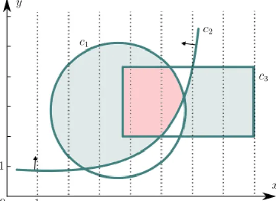
Example 3. Figure2.2describes three constraints c1, c2, and c3 over two variables x and y. Geometrically speaking, constraint c1 defines a disc, c2 is an upper half-space, and c3 is a rectangle. Thus, c1 can be expressed by a quadratic inequality, c2 by a non-linear inequality, and c3 by a conjunction of four linear inequalities. The pink zone contains all the solutions of the CSP _C1 with constraints c1, c2, c3 over variables x, y with respective domains [0, 8] _{✓ R, and [0, 6] ✓ R. One may also consider the CSPs C}2 and C3 which respectively contain the constraints c1^ (c2_ c3) and c1 , (¬c2^ c3) producing different solution areas (i.e., solution spaces/feasible regions).

2.2.3 Satisfaction and Optimization Problems

A constraint satisfaction problem consists in determining if a constraint satisfaction pro-gram (cf. Definition 2.2.1) is either satisfiable or unsatisfiable. Formally, a valuation v satisfies a CSPP = (X, D, C) iff there exists a valuation v over variables X satisfying all the constraints in C (i.e., the set of constraints in C is interpreted as a conjunction of constraints). If such a valuation v exists we say that P is satisfiable (and v is named a solution ofP), otherwise we say that P is unsatisfiable.

(25)

16 Chapter 2. Constraint Programming Real var. Integer var. Mixed var. Finite var.

Linear P NP-complete NP-complete NP-complete Non-linear decidable undecidable undecidable NP-complete

Table 2.1: Complexity for the Constraint Satisfaction Problem Classes containing Linear and Non-Linear Constraints Problems over Real, Integer, Mixed, and Finite variables. Definition 2.2.1 (Constraint Satisfaction Program). A Constraint Satisfaction Program ( CSP for short) is a triplet P = (X, D, C) where X is a set of variables, D contains the domains associated to the variables in X, and C is a finite set of contraints over variables from X.

In the following, we call CSP family a set of CSPs sharing properties (e.g., only using integer variables, only considering linear constraints). Thus, according to a CSP family its theoretical complexity for the satisfaction problem may be polynomial or not, and either be undecidable. Table 2.1 from [7] synthesizes theoretical complexities for solving the satisfaction problem according to variables and constraints types. For instance the satisfaction of: a conjunction of linear constraints over real variables can be solved in polynomial time [8]; a conjunction of constraints over integer finite variables is an NP-complete problem [9]; non-linear constraints over unbounded integer variables is an undecidable problem [7].

2.2.4 Constraint Modelling

Given a problem to answer, the objective of constraint modelling is to encode the problem to be solved into a constraint program such that a solution of the constraint program can be translated into a solution of the original problem. Definition 2.2.2 recalls the concept of CSP modelling. Constraint modelling is presented in Definition 2.2.3. In order to construct a constrain program _P0 _{modelling a constraint based problem} _{P one must} find a correspondence relation linking the valuations satisfying_P0 _{with the configurations} belonging to_{P. Thus, if one is able to satisfy the CSP the correspondence relation ensures} the existence of a configuration belonging to the constraint based problem. Furthermore, if the correspondence relation is decidable (ideally in polynomial time), one can construct at least one valid configuration from a solution given by the CSP.

Definition 2.2.2 (Model). Let A be a set of objects, S be a set of object states, and _P be a constraint based problem. We say that the CSP (X, D, C) models _{P iff there exists} a correspondence relation _{R ✓ D}X _{⇥ S}A _s.t.

1. for each (v, v0₎ _{2 R, the valuation v satisfies C and the configuration v}0 _{belongs to} P

(26)

2.2. Constraint Modelling 17

3. for each configuration v0 _in _{P there exists a valuation v s.t. (v, v}0₎_{2 R}

Definition 2.2.3 (Modelling). Let _{L be a set of constraint based problems. We say that} M is a constraint modelling of _{L iff M is a mapping associating to each P in L a CSP P}0 s.t. _P0 _models _P.

Modelling a constraint based problem as a constraint satisfaction program can be characterized in four steps. Definition 2.2.3 requires the existence of a correspondence relation. Thus, the programmer mainly builds the CSP while taking into account the correspondence between the original problem and the developed CSP. Firstly, the pro-grammer identifies the decisions variables: i.e., the variables with a clear semantics in the problem to be solved. Secondly, she/he determines the auxiliary variables (i.e., non decision variables used for intermediates constraints/computations). Thirdly, she/he sets the domain of each variable, also called the limits of each variable in the context of in-terval based domains. Fourthly, she/he adds the constraints that must be satisfied by the variables. These four steps are not necessarily straightforward and the programmer usually refines each step until a fix point is reached: the constructed CSP models the problem to solve. The following example proposes a modelling for the n-Queens problem. Note that this is a first modelling and that we are going to improve it in the following sections.

Example 4 (Example1continued). We propose a first CSP modelling M0 for solving the n-Queens problem where the decision variables model the columns and the lines chosen for the queens. Formally, let L be the set of all the n-Queens problems with n 2 N. M0 is the mapping associating to each n-Queens problem in L the CSP (X, D, C) such that X contains one variable ci and one variable ìper queen index i2 {1, . . . , n}. These variables respectively indicate the column and the line position of the ith queen on the chessboard. Furthermore, the domain for all these variables is{1, . . . , n} and the constraints are the followings ones for each pair (i, j) of two different queen indexes: 1. queens i and j are not on the same line: ì 6= `j; 2. queens i and j are not on the same column: ci 6= cj; 3. queens i and j are not on the same diagonal: |(ì − `j)/(ci − cj)| 6= 1. Note the abstraction difference between the modelling M0 and the CSP produced by M0 which models the n-Queens problem in L with n 2 N fixed. The CSPs produced by M0 have a quadratic size in terms of n (cf. the 3⇥!n

2" constraints) and use non linear constraints over integer variables.

As in other programing paradigms (functional programming, object oriented program-ming, etc.) one problem can be written as many (syntactically) different constraint pro-grams with equivalent semantics (i.e., they are all equivalently satisfiable or unsatisfiable or they all find the same optimal solution). We discuss this problematic in Section 2.3.2.

(27)

2.2.5 Modeller.

According to the type of variables (e.g., Boolean, integer, continuous variables) and the type of the constraints (e.g., linear, convex, non-linear, global constraints) one may look for the most appropriate research axes for modelling its problem. With an objective to share a common modelling language the mathematical programming community proposed A Mathematical Programming Language (AMPL for short) [10] as an algebraic modelling language for describing CSPs. AMPL is supported by dozens of state-of-the-art tools for constraint program solving (e.g., CPLEX [11], Couenne [12], Gecode [13], JaCoP [14]). However, each research axe (each one specialized on dedicated families of CSPs) developed its proper modelling languages and tools. We present a landscape of CSPs families with their respective modelling languages and tools.

1. SAT (for Boolean Satisfiability Problem) contains CSPs with contraints over Boolean variables. The Conjunctive Normal Form (CNF for short) which consists of con-junctions of discon-junctions of literals (e.g., (x1 _ ¬x2)^ (x2_ x3) where x1, x2, and x3 are three Boolean variables) is the main practical modelling language used in this community. The DIMACS [15] format is the standard text format for CNF representation. See [16] for more details about CNF encodings.

2. LP, IP, MILP (respectively for Linear Programming, Integer Programming, and Mixed-Integer Linear Programming) contain constraint programs with respectively: linear constraints over continuous variables; linear constraints over integer variables; and linear constraints over continuous and integer variables. These three families are identified as mathematical programming languages. Formally the constraint programs of these families are presented in the following form: Ax b where x is a column vector of variables with height n, and A 2 Rm,n _{and b} _{2 R}m,1 _{are two} matrices of coefficients. This encodes m inequalities over n variables. [17] recalls various modelling technics and use for these CSPs families.

3. FD (for Finite Domain Programming) contains constraint programs with constraints over variables with finite domains. There is no restriction on the constraints types. They can be linear, convex, non convex, non-linear such as trigonometric functions, exponential. There are also richer constraints expressed in the form of predicates, known as global (or meta) constraints which have been identified for their expressive-ness (e.g., all-different, element, global-cardinality) and help the solution process (cf. Section 2.3.1). See the Global Constraint Catalogue for more details [18]. Finally, there are two main formats for representing CSPs (XCSP3 [19] and FlatZinc [20]) each one associated with a constraint modeller (resp. MCSP3 [21] and MiniZinc [22]). While this CSP family allows any logical combination of constraints (negation, disjunction, implications, etc.) FD solvers are called propagation based solvers and are specialized for solving conjunction of constraints [23].

(28)

2.3. Constraint Solving 19

4. SMT (for Satisfiability Modulo Theory) allows any logical combinations of constraints over continuous and integer variables. The satisfiability stands for the logical com-bination of constraints while the theory stands for the semantics of the combined constraints. The logical combination of constraints can use any logical constraints (i.e., conjunction, disjunction, negation, implication, equivalence). Theories range from linear-constraints to non-linear constraints with integer, real-number, Boolean, or any combination of these types (even bit vectors and floating-point numbers). The SMT-LIB format [24] is the standard format for representing CSP from this family. This norm also describes all the standard theories and their dependencies. SMT is more general than SAT, IP, LP, MILP. See [25] for an introduction to and applications of SMT.

Example 5 (n-Queens Problem Continued). We proposed in Example4the modelling M0 for solving the n-Queens problem. This modelling can be transformed into a linear integer modelling M1 producing CSPs from the IP family by replacing the non-linear constraints |(ì− `j)/(ci− cj)| 6= 1 by the constraints ì− `j 6= ci− cj and ì− `j 6= cj− ci. Further-more, this modelling can be transformed into a FD modelling M2 by replacing the 2⇥

!n 2 "

constraints ensuring the “no threat” requirement by lines and columns with the only two following constraints: all-different(`1, . . . , `n) and all-different(c1, . . . , cn). Thus, M2 models are smaller than those from M0 and M1 Consider the 5-Queens problem. M0, M1, and M2 respectively produces 30, 40, and 22 constraints and have 10 variables. In addi-tion to having less constraints, the models produced by M2 use the all-different global constraint which ensures faster resolution than the use of a clique of binary inequality constraints.

Example 5 illustrates how our n-Queens problem can be supported by the IP and the FD families. Thus, a constraint based problem can be modelled as many constraint programs such that each one can be targeted to possibly different constraint satisfaction program families. In the next section we explain how the different CSPs families are solved.

2.3 Constraint Solving

In this section we give an overview of CSP solving. While we presented in the previous section various CSP families for modelling constraint based problem, we present in this section how these families are solved in practice.

Remark We present in this section some general methods for solving the CSPs families presented previously. However, before using the general solution one may also check if its problem does not belong to a subfamilies with practical/theoretical advantages.

(29)

20 Chapter 2. Constraint Programming For instance, SAT community uses the Post’s lattice for differentiating clones of Boolean functions for whose the satisfaction problem is in P or in NP [26]. In FD these complexity differentiation are dichotomy theorems, one famous is the Schaefer’s dichotomy theorem [9]. Finally, in the non-linear programming context, the quadratic convex programming is in lower complexity class than non-linear programming [27].

2.3.1 Satisfaction

In the general case, the combinatorics implied by the relations between the variables in the constraints makes a CSP hard to solve. In practice, complete solvers need to explore the search space (i.e., the set containing all the valuations). This is performed by branch and reduce algorithm where the search space is explored by developing a dynamic tree construction. Each node in the tree corresponds to a state in the exploration process (i.e., a succession of choices/decisions leading to a partial valuation of the variables and/or a reduction of the domains size and/or the adjunction of learned knowledges, etc.). Thus, a path from the root to a leaf recursively cut the search space into smaller search spaces until the satisfiability or the unsatisfiability is proven [28, 29]. The search starts from the root node which consists of the original CSP to solve (i.e., all the valuations are candidates possibly satisfying the CSP). Then, for each node in the tree exploration process the algorithm starts by reducing the current search space. This mainly consists in applying inferences rules such as resolution rules, computing consistency in order to reduce the search space while preserving all the valuations satisfying the CSP. Thanks to these reductions the next step checks if the reduced CSP is trivially satisfiable or unsatisfiable (e.g., the CSP has been syntactically reduced to a tautology, a contradiction, an empty set of constraints, etc.). If the CSP is trivially satisfiable, then a valid valuation can be found (mainly by reading the domains which has been reduced thanks to the successive cuts). containing the decisions history. If the CSP is trivially unsatisfiable, then this exploration path is closed and the exploration process carries on in an other opened exploration path. Otherwise, the current state space is split into possibly 2, 3, . . . , n smaller search spaces and the exploration process will be evaluated for each smaller CSP instances.

Algorithm 1 recalls this generic search strategy. The two main generic functions are reduce and splitSearchSpace which respectively reduces the search of the CSP while preserving all the valuations satisfying it (i.e., this function may only remove unsatisfying valuations), and split the current CSP in many k CSPs (with a possibly different k 2 N at every loop iteration) such that the union of their search spaces cover the whole search space of the split CSP (it is not required to perform a partitioning and sub-problems may share valuations). Also, we considered here a queue as a CSP buffer but a more sophisticated object may be used to select dynamically the next buffered CSP to the treated. The algorithm stops when it finds a valuation satisfying one sub-problem. We now discuss how this generic is implemented for treating CSPs from various famillies.

(30)

1: function satisfaction(P = (X, D, C) : CSP) return Map<X,D> 2: queue : Queue<CSP> 3: _P0 : CSP 4: 5: queue.add(P) 6: while not(queue.empty()) do 7: _P0 _queue.pop()

8: # Reduces the CSP while preserving all solutions 9: _P0 _reduce(P0)

10:

11: # Case the CSP is trivially satisfiable after reduction: returns a sat valuation 12: if isTriviallySat(_P0_{) then}

13: return findValuation(_P0₎ 14:

15: # Case the CSP is trivially unsatisfiable after reduction: ignores it 16: else if isTriviallyUnsat(_P0_{) then}

17: continue

18:

19: # Else split the current CSP in “smaller” CSPs and add them to the queue

20: else 21: queue.addAll(splitSearchSpace(P0)) 22: 23: end if 24: end while 25: 26: return ; 27: end function

Algorithm 1: Generic Algorithm for Solving Constraint Satisfaction Problems

• In the SAT community the DPLL algorithm [30] corresponds to the instantiation of splitSearchSpace by the selection of a non-instantiated variable x (i.e., a variable x with domain _{{true, false}) and to the construction of two CSPs such that} the first one contains the clause x and the second one contains the clause _{¬x. Then,} the reduce function performs unit propagation and pure literal elimination. The isTriviallySat function checks if constraints form a consistent set of literals and isTriviallyUnsat function checks the emptiness of the set of constraints.

• In the FD community, the constraint propagation with backtracking method consists in instantiating splitSearchSpace and reduce in the following way. In general, splitSearchSpace starts by selecting a non-instantiated variable x. Then, it con-structs one CSP per value k in the domain of x such that each constructed CSP is derived from the current CSP by setting the domain of x to the singleton domain {k}. We call search strategy a heuristic returning for a given CSP the next vari-ables and domain values to use in order to realize the split search. On the other

(31)

22 Chapter 2. Constraint Programming hand, the reduce function performs propagations by calling filtering algorithms and computing consistencies (e.g., node consistency, arc consistency, path consis-tency). Informally, a filtering algorithm removes values that do not appear in any solution. Global constraints usually come with dedicated filtering algorithms em-powering the propagation process. Finally, the isTriviallySat function checks if the instantiated variables satisfy all the constraints and the isTriviallyUnsat function checks if a constraint is violated or if a variable domain becomes empty. See [23] for more details.

• The branch-and-reduce framework used for solving non-linear programs with con-tinuous variables, for instance HC4 [31], corresponds to instantiate in Algorithm 1 the function splitSearchSpace by the branching function (e.g., select a variable x with domains [a, b] _{✓ R and a real number c 2 [a, b] in order to construct two} CSPs which respectively contain the constraints x _{ c and x ≥ c), the reduce} uses reducing consistencies in order to filter domain variables while preserving so-lutions. Finally, the isTriviallySat function guesses a valuation satisfying all the constraints for tight domains and the isTriviallyUnsat function checks if a constraint is violated or if a variable domain became empty.

• The SMT community gathers solving techniques from various CSP families. Indeed, a SMT instance is considered as the generalization of a Boolean SAT instance in which various sets of variables are replaced by predicates (e.g., linear or non-linear expres-sions for continuous variables, integer constraints). Thus, the splitSearchSpace enumerates solutions of the SAT instance abstracting the CSP to solve (i.e., each constraint which is not a Boolean function is replaced by a unique Boolean variable). Then, each solution of the SAT instance is translated into a set of constraints which leads to a conjunction of constraints, each one being a sub-problem to be solved. According to the theory of this sub-problem (linear programming, integer program-ming, etc.) proper methods from the corresponding CSP family are used. This approach, which is referred to as the eager approach loses the high-level semantics encoded in the predicates. Actual SMT solvers now use a lazy approach solving par-tial SAT sub-problem and then answering their corresponding predicate parts while constructing a global solution [32]. In SMT, we call strategy an implementation/con-struction of the splitSearchSpace and reduce functions.

Furthermore each community (i.e., SAT, FD, etc.) provides many tools which imple-ment the generic Algorithm 1. The performance of these tools is mainly due to their implementation of the reduce and splitSearchSpace functions inherited from years of research next to the practical resolution of real world problems. This includes the study and the availability of wide variety of concrete heuristics [33] and search strategies [34] eventually branched with an offline or online learning (e.g., no good, learned clauses). In

(32)

this thesis we focus on constraint modelling of constraint based problems and on domain reducing functions called propagators implemented in the reduce function.

We presented independently how various CSPs families tackle the solving problem. However, some research has been realized in order to make them collaborate. For instance, the finite domains CSP family met continuous domains CSP family while preserving global constraints by linking CHOCO and IBEX solvers [35]. Also, the integration of both IP and FD has been discussed helping to design a system such as SIMPL [36]. On the other hand, we already mentioned the fact that the SMT community uses solving techniques for clearly identified theories. In the same time, they started to include global constraints from FD and [37] shows how the all-different constraint can be supported by SMT solvers which offers promising results. Finally, in [38] the authors develop cooperative constraint solver systems using a control-oriented coordination language. This work has been used for solving non-linear problems [39] and interval problems [40] as well.

We presented here a generic complete algorithm answering the constraint satisfaction problem. Such complete method always returns a valuation satisfying the given CSP if it exists and returns none if such valuation does not exist. Thus, an incomplete algorithm may not be able to indicate if the CSP is unsatisfiable but may find a valuation satisfying the constraint program. We consider complete solvers in this thesis.

2.3.2 Improving Models

As said in the modelling section there is more than one CSP which encodes a given con-straint based problem. Furthermore, the time required for solving these equivalent CSPs may differ from one to another with possibly an exponential gap. We present here various methods exploring how CSPs can be improved for reducing solving time: reformulation, symmetry-breaking, redundant constraints, relaxation, and over-constraint. In all cases these improvements can be performed by hand. However, solvers may implement them for automatic uses.

Definition 2.3.1 (Reformulation). LeC be a CSP. A reformulation ⇢ transforms a CSP C into a CSP C0 _{s.t. all the solutions of} _{C can be mapped to a solution in C}0 _{and all the} solutions ofC0 _{are translatable as a solution} _{C. Thus, C}0 _{models the same problem than} _C. There exists model transformations for transposing a CSP from a family to another one. Definition2.3.1recalls the concepts of reformulation, i.e., how to produce a new CSP from an existing CSP modelling the same contraint based problem. A low level constraint language such that the Conjunctive Normal Form (i.e., a Boolean functions expressed as conjunctions of disjunctions of literals) language used in the SAT community is now tractable with SAT state-of-the-art solvers for millions of variables and constraints [41]. In some cases reformulating a satisfaction problem into a lower constraint language may offer better resolution times. For instance in [42], the authors reformulate their modelling

(33)

24 Chapter 2. Constraint Programming from CP to SAT which highly increases the sizes of the CSP. But the first modelling is not solved by CP solvers while the second one is solved by SAT solvers.

Example 6 (n-Queens Refomulation). Consider the modelling M2presented in Example5. Recall that the “no threat” rule for diagonals is managed by the constraints ì−`j 6= ci−cj and ì− `j 6= cj− ci considered for each pair of two different queen indexes i and j. These constraints are equivalent to ì − ci 6= `j − cj and ì + ci 6= `j + cj. Since they must hold for each pair of two different queen indexes, all these constraints can be replaced by the two all-different global constraints. Since the all-different constraint support variables as inputs we create the auxiliary variables xi and yi for all i 2 {1, . . . , n} such that xi = ì − ci and yi = ì + ci. Thus, the constraints expressing the “no threat” rule for diagonals can be replaced by the two constraints all-different(x1, . . . , xn) and all-different(y1, . . . , yn). We call M3 this modelling derived from M2. M3 is called a reformulation of M2. M3 models contain n + 3 constraints whereas M2 models contain a quadratic number of constraints in term of the number of queens n. Note that a reformulation may also change the variables and their domains and is not restricted to constraint modifications.

Definition 2.3.2 (Symmetry). Le P be a constraint based problems over a set of objects A with states S. We say that P contains symmetries iff there exists a permutation σ of the set of configurations s.t. P is stable by σ. (i.e., σ(c) 2 L, for all c 2 L ✓ SA _s.t. L ⌘ P.)

A symmetry in a constraint based problem is a permutation of the configurations in the problem (cf. Definition 2.3.2). Thus, symmetry breaking consists in taking advantages of symmetry detection in constraint based problem to only model a subset of all the configurations in the problem, i.e., to only model the configurations which can not be obtained by symmetries. Symmetry breaking reduces the size of the search space and therefore, the time wasted in visiting valuations which are symmetric to the already visited valuations. The solution time of a combinatorial problem can be reduced by adding new constraints, referred as symmetry breaking constraints. We invite the reader to consider [43] for more details.

Example 7 (n-Queens Symmetry Breaking). Consider the modelling M3 presented in Example 6. Let n be a fixed number of queens and C be the CSP produced by M3 for the n queens problem. Note that in C the n queens are unordered: i.e., all the queens are totally identical. Thus, for any valuation solution of C one may interchange the val-ues (`i, ci) representing the position of the ith queen with the values (`j, cj) representing the position of the jth queen to obtain another valuation solution of C. We construct a new modelling, named M4, ordering the queens and realizing some symmetry breaking. M4 is such that for each n 2 N its corresponding CSP model (X, D, C) for solving the

(34)

n-Queens problem contains the ci variables with domain {1, . . . , n} and no variable ì. Similarly to the previous modellings the ci variables represent the column position of the queens. However, in this modelling each ci with i 2 {1, . . . , n} is fixed with a line, the ith line. Thus, ci contains the column position of the queen on the ith line and there are no more ì variables in M4. The constraints xi = ì − ci and yi = ì + ci from M3 are respectively replaced by xi = i− ci and yi = i + ci in M4 for all i 2 {1, . . . , n}. To sum up, the constraints in C are the following ones: all-different(c1, . . . , cn), all-different(x1, . . . , xn), all-different(y1, . . . , yn), xi = i− ci and yi = i + ci for all i 2 {1, . . . , n}. Note that this modelling still contains symmetries (e.g., chessboard rotations, chessboard plane symmetries). For instance setting the domain of the variable c1 to {1, . . . , dn/2e} removes some chessboard plane symmetries.

Definition 2.3.3 (Redundancy). Let C be a CSP and c be a constraint over a set of variables X. We say that c is a redundant constraint for C iff adding the constraint c to the CSP C does not change the solution space of C.

In a general context minimizing the number of constraints (and/or the number of variables) in a CSP does not necessary implies lower solving time in practice. We call redundant constraint a constraint which does not change the set of valuations satisfying a given CSP when adding this constraint to the CSP (cf. Definition 2.3.3). In practice adding well chosen redundant constraints may speed up the solving process, or obtain a scale up (see [44] for instance). However, in the linear programming case detecting redundant constraints in order to remove them may accelerate the resolution process (see [45] for more details).

Definition 2.3.4 (Relax & Over-constrain). LetP be constraint based problem over a set of objects A and a set of states S. Let C be a CSP. We say that C is:

• a relaxed modelling of problem P iff there exists a constraint based problem P0 s.t. CSP _{C models problem P}0 _{and all the configurations in} _{P belongs to P}0_;

• an over-constrained modelling of problem P iff there exists a constraint problem P0 s.t. CSP _{C models problem P}0 _{and all the configurations in} _P0 _{belongs to} _P.

As last modelling strategies we present the relaxation and the over-constrain cases (cf. Definition 2.3.4). A relaxation is an over-approximation of a difficult problem by a nearby problem that is easier to solve. For instance a relaxation may transform integer variables into real variables (indeed this produces a greater solution space), or may only consider a convex hull of the problem by using only linear inequalities (e.g., [46]). An over-constrain model is an under-approximation. This consists in modelling a constraint based problem contained by the original problem to solve. Thus, by reducing the size of the search space, one may hope a gain in term of resolution time (see [47] for instance).

(35)

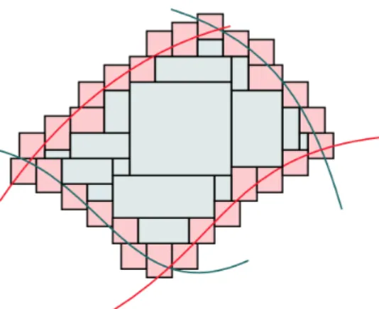
Figure 2.3: Box Paving for a Constraint Satisfaction Problem. Gray boxes only contain solutions. Pink boxes contains at least one solution. The union of the gray and the pink boxes covers all the solutions.

2.3.3 Real numbers vs. Floating-point numbers

As presented previously, one common variable domain for modelling is the real-numbers domain, written R. When using this domain one expects that the solver takes into account the classical arithmetic properties verified by R (e.g., associativity, commutativity, infinite limits, etc.). In practice, computer scientists use floating-point numbers for simulating real numbers. Floating-point numbers represent a finite numbers of real numbers with finite (binary) representation. The IEEE 754 norm [48] is now considered as the norm for representing floating-point numbers in programs. This norm encodes 232 _{finite real} numbers where the smallest non-zero positive number that can be represented is 1⇥10−101 and the largest is 9.999999⇥ 1096_{, the full range of numbers is}_{−9.999999 ⇥ 10}96 _through 9.999999⇥ 1096_{; it contains two signed zeros +0 and}_{−0, two infinities +1 and −1, and} two kinds of N aN s. In the following we write F for the set of real-numbers representable in the IEEE 754 norm.3 _{The first notable fact is that floating-point arithmetic (i.e.,} arithmetic over F) is not equivalent to real number arithmetic (i.e., arithmetic over R). Precision limitation with floating point numbers implies rounding: a real-number x 2 R which is not in F is rounded to one of the neartest floating-point number. The IEEE 754 norm describes five rounding rules (two rules round to a nearest value while the others are called directed roundings and round to a nearest value in a direction such as 0, +1, −1). For instance: 0.110 (number 0.1 represented in base 10) does not have a finite representation in base 2 and thus, it does not belong to F; there exists floating-point numbers x2 F s.t. x + 1 = x in the floating-point arithmetic.

Implementing real number arithmetic in CSP solvers is challenging. Recall that we presented CSP valuation solutions as a mapping from the variables to their respective do-mains. Since some valuations to R may not be representable with floating-point numbers, solvers like RealPaver [49] find reliable characterizations with boxes (Cartesian product of

3

(36)

intervals) of sets implicitly defined by constraints such that intervals with floating point bounds contain real-number solutions. Thus, the real number valuation solutions are bounded by the interval valuation solutions.

(37)

(38)

29

Chapter

3

Program Verification

30 Chapter 3. Program Verification Since softwares take more and more control over complex systems with possibly critical impact on the society (e.g., car driving software, automatic action placements, ...) the verification community develops methods for ensuring the validity of such programs. After introducing in a first section the main objectives of program verification, we go deeper into the two verification fields concerned by our contributions. Our first contribution relates to Abstract Interpretation and the second one considers Model Checking for Markov chains. Finally, we present a brief overview concerning how constraint programming meets verification problems.

Warning. We choose the word “program” for system change descriptions while the verification community also uses the word “model” with the same signification. Recall that we already introduced the word “model” in the constraint programming background (cf. Section 2.2). Thus we reserve it for the constraint context.

3.1 Introduction

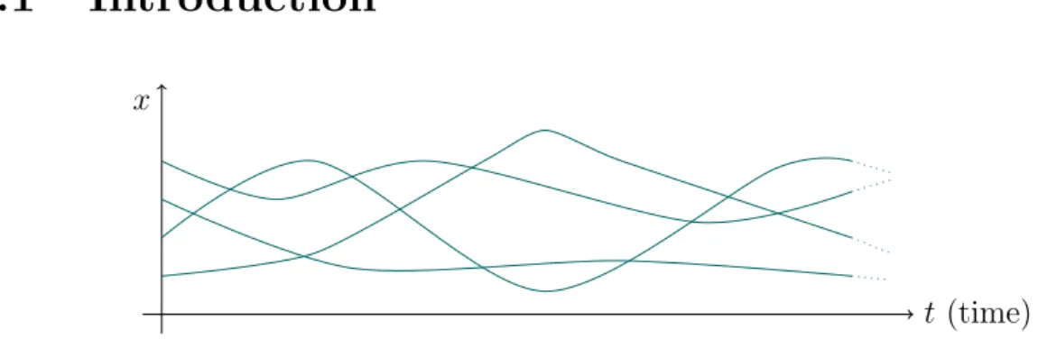
t (time) x

Figure 3.1: Instance of four possible traces of a variable x while executing the same program.

We focus in this thesis on program verification problems, i.e., we do not consider hardware verification problems. In this context, the word “program” refers to a com-puter science program written in a dedicated programming language [50]. There is a wide variety of programming languages which can be grouped by programming paradigms: functional programming (e.g., Javascript, Python), object oriented programming (e.g., C++, Java), reactive programming (e.g., FAUST, LUSTRE), probabilistic programming (e.g., ProbLog, RML), etc. Even if these languages may have different programming approaches they all share the same verification expectations. Indeed, whatever the lan-guage, a program is designed to be executed (in our concern we consider that programs are executed on a machine with memory). We briefly recall some vocabulary proper to program verification. We call run an execution of a program. During a run the machine memory varies over the time. We call state a snapshot of the memory at a given time. Finally, a trace is the succession of states corresponding to a run of the program. Thus, program verification consists in analyzing traces in order to determine if a given property