April 29, 2014
The PLATO Simulator: modelling of high-precision high-cadence
space-based imaging
?
P. Marcos-Arenal
1, W. Zima
1, J. De Ridder
1, C. Aerts
1,2, R. Huygen
1, R. Samadi
3, J. Green
3, G. Piotto
4, S. Salmon
5,
C. Catala
3, and H. Rauer
6,71 Instituut voor Sterrenkunde, KU Leuven, Celestijnenlaan 200D, 3001 Leuven, Belgium e-mail: [email protected]
2 Department of Astrophysics, IMAPP, Radboud University Nijmegen, 6500 GL Nijmegen, The Netherlands
3 LESIA, Observatoire de Paris, CNRS UMR 8109, UPMC, Universit´e Denis Diderot, 5 Place Jules Janssen, 92195 Meudon Cedex, France
4 Dipartimento di Astronomia, Vicolo dell’Osservatorio 5, 35122 Padova, Italy
5 Institut d’Astrophysique et de G´eophysique de l’Universit´e de Li`ege, All´ee du 6 Aoˆut 17, 4000 Li`ege, Belgium
6 German Aerospace Center (DLR) Institut f¨ur Planetenforschung Extrasolare Planeten und Atmosph¨aren, Rutherfordstraße 2, 12489 Berlin, Germany
7 TU Berlin, Hardenbergstr. 36, 10623 Berlin, Germany Received ; Accepted
ABSTRACT
Context.Many aspects of the design trade-off of a space-based instrument and its performance can best be tackled through simulations
of the expected observations. The complex interplay of various noise sources in the course of the observations make such simulations an indispensable part of the assessment and design study of any space-based mission.
Aims.We present a formalism to model and simulate photometric time series of CCD images by including models of the CCD and its electronics, the telescope optics, the stellar field, the jitter movements of the spacecraft, and all of the important natural noise sources.
Methods. This formalism has been implemented in a versatile end-to-end simulation software tool, specifically designed for the PLATO (Planetary Transists and Oscillations of Stars) space mission to be operated from L2, but easily adaptable to similar types of missions. We call this tool PLATO Simulator.
Results.We provide a detailed description of several noise sources and discuss their properties in connection with the optical design, the allowable level of jitter, the quantum efficiency of the detectors, etc. The expected overall noise budget of generated light curves is computed, as a function of the stellar magnitude, for different sets of input parameters describing the instrument properties. The simulator is offered to the scientific community for future use.
Key words.Instrumentation: detectors – Techniques: image processing – Methods: data analysis – Asteroseismology – Planets and
satellites: detection
1. Introduction
Recent uninterrupted long-term µ-mag-precision space photom-etry opened a new era in time-domain astronomy and has led to numerous exoplanet detections, see, e.g., Moutou et al. (2013) for a review of CoRoT (Convection, Rotation and planetary Transits) results and Borucki et al. (2010); Welsh et al. (2012); Batalha et al. (2013) for results obtained from the Kepler mis-sion. As a by-product, both space missions also implied a gold-mine for stellar variability studies (e.g., Debosscher et al. 2009; Sarro et al. 2009; Prˇsa et al. 2011; Debosscher et al. 2011). In particular, detailed seismic probing was finally reached and gave new insights into the physics of stellar and galactic struc-ture, pointing out limitations of standard models (e.g., Degroote et al. 2010; Beck et al. 2012; Miglio et al. 2012, 2013). Even tests of stellar evolution theory for a wide variety of stel-lar masses and evolutionary stages, through asteroseismic data alone or combined with ground-based data, became possible thanks to dedicated CoRoT and Kepler asteroseismology pro-grammes (e.g., Michel et al. 2006; Gilliland et al. 2010; Bedding
?
Software package available at the PLATO Simulator web site (https://fys.kuleuven.be/ster/Software/PlatoSimulator/).
et al. 2011) and from multivariate statistical studies based on seismic, polarimetric, and spectroscopic data (e.g., Aerts et al. 2014). Asteroseismology of eclipsing binaries (e.g., Maceroni et al. 2009; Welsh et al. 2011; Tkachenko et al. 2014; Beck et al. 2014) and of exoplanet host stars (e.g., Gilliland et al. 2011; Chaplin et al. 2013; Huber et al. 2013b,a; Van Eylen et al. 2014) only became possible in the current space photometry era.
Despite the availability of these numerous CoRoT and Kepler data sets with long time-base, new projects for similar studies are in development. These new studies are capable of mapping the entire sky rather than just a small portion of it, as was the case for CoRoT and Kepler. The current paper concerns the PLATO2.0 mission (hereafter simply called PLATO), which was recently accepted as M3 mission in the Cosmic Vision 2015 – 2025 programme of the European Space Agency (ESA). PLATO is an acronym for PLanetary Transits and Oscillations of Stars and is a mission that will operate from the second Lagrange point (L2) of the Sun-Earth system.
PLATO’s goals are to study the formation and evolution of planetary systems, with specific emphasis on Earth-like planets in the habitable zone of bright solar-like host stars. PLATO will have the capacity to detect and characterize hundreds of
like planets and thousands of larger planets with the photomet-ric transit technique already used by CoRoT and Kepler. Up to 1 000 000 stars will be observed and characterized over the course of the full mission. Masses, radii, and ages of 80 000 dwarf and subgiant stars will be measured with sufficient pre-cision to allow for their asteroseismic modelling. The expected noise level for stars with visual magnitudes of less than 11 is 34 ppm per hour, and for stars brighter than 13th magnitude the noise is expected to be below 80 ppm per hour. A unique feature of PLATO compared to previous and other planned space mis-sions is its capacity to measure a fraction of the targets in two photometric bands.
In order to achieve its scientific aims, PLATO is equipped with 34 12 cm aperture telescopes and 136 CCDs (four CCDs per camera) with 4510×4510 18 µm pixels, to cover about 50% of the sky, operating in the 500-1000 nm spectral range. Each se-lected target is assigned a 6×6 pixel window to produce its light curve on board. This on-board processing is required to limit the amount of data to be downloaded to ground for its wide field of view (FoV). Detailed descriptions of the PLATO M3 mission are available in Rauer et al. (2013) and in the Yellow Book submit-ted to ESA for the selection of M3 (ESA 2013)1.
PLATO’s cameras are high-precision imagers whose ex-pected performance must be carefully assessed from an appro-priate overall instrument model. The instrument noise perfor-mance cannot be derived from the simple addition of the noise properties of the individual contributors due to the complex in-teraction between the various noise sources. As is often the case, it is not feasible to build and test a prototype of the PLATO imag-ing devices. Hence, numerical simulations performed by an end-to-end simulator are used to model the noise level expected to be present in the observations. Such simulations not only allow us to study the performance of the instrument, its noise source response, and the data quality, but they are also an essential tool for the fine-tuning of the instrument design for different types of configurations and observing strategies. The simulator should also allow us to test the scientific feasibility of an observing pro-posal. In this way, a complete description and assessment of the expected objectives of the mission can be derived.
In this paper, we present a formalism, termed PLATO Simulator, to model each of the noise sources affecting a space-based high-resolution imager and the mutual interaction of these noise sources. The performance of previous space photometers, such as MOST (Walker et al. 2005), CoRoT (Auvergne et al. 2009), and Kepler (Koch et al. 2010; Caldwell et al. 2010) have been tested and evaluated using approaches specifically designed for each of these missions alone, keeping in mind their orbit (low-Earth in the case of MOST (Microvariablity and Oscillations of Stars) and CoRoT and Earth-trailing for Kepler). Our aim is to provide the scientific community with a tool that is easily adaptable for other high-precision photometric space missions, taking PLATO as the case study to illustrate our simulator. Our approach here is based on previous work developed in this spirit for the MONS (Measuring Oscillations in Nearby Stars) and Eddington mission projects, which never made it to implementation phase (De Ridder et al. 2006, here-after termed DAK06). We have further developed and imple-mented this formalism in the PLATO Simulator end-to-end sim-ulation software-tool, which was specifically constructed for the PLATO assessment and Phase A/B1 studies, but is easily adapt-able to other missions.
1 http://sci.esa.int/plato/53450-plato-yellow-book/
In the following section, we describe each of the noise sources and the algorithms developed to model them, as well as their implementation and interaction. We introduce the PLATO Simulator in Sect. 3 and, finally, in Sect. 4, we present applica-tions of the simulator to the study of white noise and jitter for the PLATO mission. These results were used to predict the quality of its photometry to assess the transit and stellar variability detec-tion capability and to provide essential feedback for the mission design.
2. Imaging simulation
A previous preliminary version of the simulator (Zima et al. 2010) has now been completely rebuilt. It relies on new archi-tecture, to make it adaptable to other missions as well. The tech-nical details and motivation of the new architecture were already described in Marcos-Arenal et al. (2013), to which we refer the interested reader, and are therefore ommitted here.
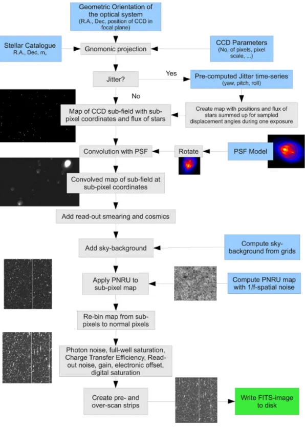
The new PLATO Simulator generates synthesized images by simulating the acquisition process of a space-based detector in-strument as realistically as possible. Each image is numerically modelled, based on a number of input parameters, which de-fine the set-up of the CCD and its electronics, the properties of the optical instrument, the FoV, the point spread function (PSF), the pixel response non-uniformity (PRNU) and all related noise sources. The process of image generation can be classified ac-cording to the sequential order shown in Fig. 1. The following subsections will give a detailed description of each of these pa-rameters:
– Imaging FoV:
CCD rotation and resizing; The CCD sub-pixel matrix; Mapping stars on the CCD; High-energy particle hits; – Satellite jitter;
– PSF Convolution;
– CCD Sensitivity variations: PRNU; – Noise effects:
Read out smearing; Sky background; Photon noise;
Electronic noise sources.
This subdivision is based on the processing chain of the whole simulation, whose schematic flow diagram is shown in Fig. 1.
2.1. Imaging FoV
A set of input parameters is required to generate a complete syn-thetic CCD image. This set of parameters defines general prop-erties of the telescope and the focal plane, the orientation of the stellar field, and the properties of the simulated time series, such as the exposure time and the number of exposures to be com-puted. To model the CCD frame, the detector characteristics are taken as inputs in terms of frame size, pixel size, and pixel scale, as well as the right ascension and declination centre of the op-tical axis, the CCD orientation, the focal plane coordinates, and the focal plane orientation.
2.1.1. The CCD rotation and resizing
To capture a concrete field, a star catalogue is required as in-put to time series project the positions of the stars on the CCD.
Fig. 1: Processing steps that are applied in the simulator to model a CCD image of a stellar field, in sequential order.
We used a gnomonic projection of the sky onto the focal plane, as described below. The orientation of the optical axis (αOAand
δOA) defines the centre of the projection. The CCD is not
nec-essarily centred on the optical axis and the focal plane has an arbitrary orientation. The position of the origin (left corner of read-out strip) of a CCD and its orientation in the focal plane
can be arbitrarily defined. The geometry of this step is depicted in Fig. 2.
For computational reasons, the full 4510×4510 pixels CCD image is generally not calculated in the PLATO simulations. Instead, we compute only a sub-field with a dimension of a few
Focal Plane Read -out CCD North γCCD (0,0) yFP xFP x γFP xCCD yCCD (∆xCCD,∆yCCD) x y FP
Fig. 2: Definition of the focal plane orientation and relative CCD location and orientation. The focal plane is rotated by the angle γFPwith respect to the north-direction. The origin of the CCD
in the focal plane is defined by its offset (∆xCCD,∆yCCD) in mm
from the centre of the focal plane. It is then rotated by the angle γCCDaround its origin.
hundred square pixels2. This sub-field, as presented in Fig. 3,
is the synthetic image to be written in a FITS (Flexible Image Transport System) file. To explore different parts of the CCD, separate simulations with different sub-field coordinates and PSFs have to be carried out. Due to the PSF, the brightness of stars close to the outer margins of the frame affects the pixels close to the inner margins of the frame. To ensure the inclusion of the flux of these sources, we take an offset margin around the frame into account.
2.1.2. The CCD sub-pixel matrix
A CCD consists of a two-dimensional rectangular array of a few million pixels, which converts the energy released by the pho-ton hits into electron counts. Although the pixels typically have a physical size of only a few µm square, it is necessary to divide each pixel into sub-pixels during the simulations to correctly characterize motions smaller than one pixel. Hence, the intra-pixel sensitivity variations can be approximated by subdividing each pixel into a number of sub-pixels. The degree of accuracy increases with the number of sub-pixels. For typical simulations including jitter pointing variations, we use 128 × 128 square sub-pixels to obtain reliable results. At the end of the image genera-tion, the array is re-binned to normal pixel space.
The sub-field is the final image generated; it is a part of the CCD that is modelled in detail by the PLATO Simulator and written to FITS files (see Fig. 3). The read-out smearing effect has to be taken into account for frame-transfer CCDs with an electronic shutter, as is the case for the PLATO mission. Stars on the CCD that are outside the sub-field contribute to read-out smearing on the sub-field. Also, the edge pixels of the sub-field are affected by stars that are just outside the visible field because 2 When 128 sub-pixels are considered, a 100 × 100 pixel field con-tains (100 × 128)2= 163 840 000 sub-pixels, which results in a 1.3 GB memory consumption in double precision computations. During convo-lution with the PSF, even more memory has to be allocated.
Ch ar ge Tr an sf er D ire ct ion
Read-out Register Direction
(0,0)
CCDSizeX
CCDS
ize
Y
Fig. 3: Schematic presentation of the sub-field (field of view) and the parameters required to define it. The parameters xsand ysare
the pixel coordinates of the origin of the sub-field relative to the CCD.
of their PSFs. The image convolution with the PSF is made for a sub-field that is enlarged by the size of the PSF. Once the con-volution process has been applied, the sub-field is cut to the size that was specified in the parameter file. This also applies for a sub-field that lies at the edge of the CCD.
We define the pixel coordinates (xi, yi) in the PLATO
Simulator with the following convention: the position of an ob-ject in fractional pixels is defined in a way that integer coordi-nates lie at the cross section of four pixels on the CCD (see also Fig. 4 in the user manual available from the PLATO Simulator3
web page).
2.1.3. Mapping stars on the CCD
Stellar positions are provided through a catalogue that lists their right ascension (α), declination (δ), and magnitude (mv). The
sub-pixel position of each star on the CCD is calculated through a gnomonic or pinhole projection that is widely used in optical astronomy (see Beichman et al. 1988) and closely reproduces the way in which light is projected through a lens (or via a mirror) onto a flat surface. We assume that the optical axis is perpendic-ular to the focal plane and denote its pointing direction in right ascension and declination as α0and δ0, respectively. The
projec-tion of a point with spherical coordinates (αi, δi) onto the focal
plane (xi, yi) can then be calculated from
xi=
cos(δi) sin(αi−α0)
cos(δ0) cos(δi) cos(αi−α0)+ sin(δ0) sin(δi)
, (1)
yi=
cos(δ0) sin(δi) − sin(δ0) cos(δi) cos(αi−α0)
cos(δ0) cos(δi) cos(αi−α0)+ sin(δ0) sin(δi)
. (2)
With this formalism, the y-axis of the focal plane coordinate system is aligned with the north direction (see Fig. 2). We then apply a rotation matrix to consider the arbitrary orientation of the focal plane. We consider that the origin of the CCD has an offset from the optical axis and may be rotated by an angle γCCD.
The position (xi, yi) of each star is rounded to its closest
sub-pixel coordinate. This will induce sampling artifacts, that can be reduced with a higher number of sub-pixels.
For an exposure time of texpseconds, the flux Fphotof each
star is computed from its magnitude mλ, the effective
light-collecting area A (in cm2), the transmission efficiency T of the optical system, the quantum efficiency of the detector Q, and the flux per second F0of a star with mλ= 0, from
Fphot= texpF0TλQλA10−0.4mλ. (3)
The value F0can be determined through numerical integration of
the stellar spectral energy distribution in the relevant wavelength (λ) range, normalized with the flux in that band pass for mλ=0.
The quantum efficiency (QE) and transmission efficiency (TE) are the values appropiate for the relevant wavelength (λ).
2.1.4. High-energy particle hits
High-energy particle hits arising from cosmic rays are a source of noise in photometric measurements. In space, where no pro-tective atmospheric shielding is present, cosmic hits are more abundant than on Earth. Estimates for the number of hits in sim-ilar detectors are around two events cm−2 s−1 for CoRoT (see
DAK06) and five events cm−2s−1for Kepler (NASA 2009). Such impacts can leave their marks with a large range of effects and shapes on the detector surface. They can saturate a single pixel or produce a streak of saturated pixels having complex shapes. We have modelled proton impacts through a two-dimensional ellip-tical Gaussian intensity distribution at sub-pixel level. For each event, the major axis of the ellipse, its central intensity, and two full widths at half maximum values (FWHM) are determined as-suming a stochastic process based on a number of input parame-ters to be defined by the user, more particularly the frequency of the events and their intensity. A sample synthesized CCD image containing a number of cosmic hits is shown in Fig. 4.
Fig. 4: Synthesized sample CCD image containing a number of cosmic hits (elongated shapes).
2.2. Satellite jitter
Ideally, the orientation of a spacecraft is perfectly stable and does not change during the monitoring of a stellar field. Unfortunately, this is never the case and small high-frequency relative pointing variations (jitter) of the spacecraft cause the im-ages of stars to move on the CCD even during single exposures. Mainly because a CCD has a non-uniform pixel response, jitter can lead to a loss of measured flux and aperture photometry can lead to systematic measurement errors. Fortunately, some meth-ods have been developed to recover systematic flux variations due to jitter (e.g., Drummond et al. 2006; Fialho et al. 2007), so that it can be corrected for whenever the centroids of the stars are precisely known.
The jitter is dominated by the reaction wheel noise, structural flexibility, and star sensor accuracy, whereas the pointing-drift error is mostly due to the thermal flexibility and variability in the solar aspect angle of the spacecraft. In order to meet the point-ing requirements for PLATO (0.2 arcsec rms over 14 hours), it is suggested that the reaction wheels are properly isolated and bal-anced, and that a model of the thermal deformation is included in the AOCS (attitude and orbit control system) where the two fast cameras will deliver a pointing error signal every 2.5 s.
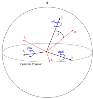
Fig. 5: Jitter configuration used by the PLATO Simulator. The jitter roll axis of the spacecraft zjis inclined by an angle λ to the
orientation of the optical axis (zC). The axis yC is normal to zC
and lies in the equatorial plane; xCis computed from yC× zC.
The effect of jitter on the CCD image of the stellar field is modelled in detail in the simulator. Jitter movements of the spacecraft can be described by the displacement angles yaw (α), pitch (β), and roll (γ). These angles are defined in such a way that zjpoints in the direction of lowest inertia of the spacecraft
and is given as angular distance from the optical axis. The axis yjis normal to zjand lies in the equatorial plane; xjis computed
from yj× zj. The orientation of the optical axis (i.e., zC) is given
in equatorial coordinates and may be different to zj. The yCaxis
lies, like the yjaxis, in the equatorial plane and is normal to zC.
Finally, xCis computed from yC× zC. The focal plane thus lies in
the xCyC-plane. Assuming that the telescope is pointed towards
objects that have an infinite distance from the CCD, any rotation of the spacecraft has the same effect on the focal plane inde-pendent of its physical distance to the jitter axis. Thus, only the angular distance of a star from the jitter axis is important.
In a next step, the focal plane coordinate system is rotated by the jitter angles around the jitter coordinate system. First, a rota-tion around xjwith the yaw angle α is carried out. This rotation
also affects the two other jitter axes, yj and zj. Next, the focal
plane is rotated around the yj-axis (already once rotated) by the
pitch angle β. This operation also rotates zj. Finally, a rotation
around the zj-axis (twice rotated) by the roll angle γ is carried
out.
The position of an object on the CCD is then calculated from a gnomonic projection on the rotated xCyC-plane. Figure 5
and focal plane reference coordinate systems. Finally, in order to match the CCD frame of reference, the x and y-axes are inverted. Therefore, a change of yaw moves the field on the CCD in the x-direction and a change of pitch moves the field on the CCD in the y-direction.
In absence of jitter motions, only one image convolution is computed and used for all subsequent exposures to compute the final image, including the considered noise sources. When jit-ter is included and modelled, an image convolution has to be computed for each exposure, evidently leading to much longer computation times.
2.3. PSF Convolution
The PLATO Simulator can read a pre-computed PSF from a file or generate a Gaussian-shape PSF to be used as the PSF mask in the sub-field. Within one sub-field, all stars are assumed to have the same shaped PSF. This is obviously an approximation due to different stellar types and because the shape of the PSF is a function of the position on the CCD.
The simulator takes into account that the shape and orienta-tion of the PSF depends on the locaorienta-tion in the focal plane. When a range of PSFs for different angular distances to the optical axis is provided, the PLATO Simulator can select the PSF that best matches the angular distance of the sub-field centre, and rotate it in such a way as to correctly orient it relative to the optical axis (see Figs. 6 and 7). Through this approach, the image distortion that should be included in the PSF pre-computed mask can be well approximated on the resulting image. It can also shift a pre-computed PSF by a fraction of a sub-pixel by bi-linear interpola-tion such that the centre of the PSF is situated at a cross secinterpola-tion. For this procedure, the centre of the pre-computed PSF has to be indicated. Figure 6 shows a 3D image of the central piece of a pre-computed PSF for PLATO, sampled in a 1024 × 1024 matrix corresponding to 8 × 8 pixels (128 subpixels per pixel) at 2.828 distance pixels from the optical axis.
X 4.2 4.4 4.6 4.8 5.0 5.2 5.4 5.6 Y 4.2 4.4 4.6 4.8 5.0 5.2 5.4 5.6 In te nsi ty 0.0 0.0001 0.0002 0.0003 0.0004 0.0005 0.0006 0.0007 0.0008
Fig. 6: Piece of a pre-computed 8 × 8 pixels PSF for PLATO at 2.828 pixels distance from the optical axis.
For the convolution of the raw stellar field, the stars are treated as point sources with sub-pixel CCD coordinates, and the
x y
Toward opt. axis
γ
Fig. 7: Definition of the orientation angle γ of the PSF towards the optical axis.
PSF are computed in Fourier space by applying a 2-dimensional fast Fourier transform (FFT). The computation of the product of the field and the PSF in complex Fourier space, followed by the conversion of the produced image to real space, is far less CPU intensive compared to performing a convolution in real space, particularly when a high number of stars occur on the sub-images and the effects of jitter have to be used in the simu-lations. The drawback is a large memory need, which limits the usable dimension of the sub-field and translates into a limit on the number of sub-pixels. For practical applications, we kept the product of the number of sub-pixels and the side length (in pix-els) of the sub-field below 6400 (i.e., 50 × 50 square pixels and sub-field at 128 × 128 square sub-pixels) for our computations on a dual-core Intel computer with 4 GB memory.
As a next step, the sub-pixel matrix, which contains the po-sitions and fluxes of all stars on the CCD, is convolved with the PSF input mask. The PSF mask should resemble the real PSF as closely as possible and thus should contain any artifacts that are due to the optical system. Also, the shape of the PSF depends on the position in the focal plane, on the wavelength range, and on the stellar type. For our simulations, a set of mono-chromatic PSFs has been calculated for different angular distances from the optical axis. From this set, we computed integrated PSFs for different stellar temperatures assuming a black-body energy dis-tribution.
The PLATO Simulator assumes that the shape of the PSF is the same over the complete sub-field. The software allows the convolution to be performed in real space or in Fourier space. Real space convolution is carried out by shifting the normalized PSF to the sub-pixel position of each star and by multiplying the sub-pixel intensity by Fphotusing the following formalism:
F(xi, yi)= i X stars Fphoti j X xPSF k X yPSF (xi− xj, yi− yk). (4)
The PSF mask is particularly important in the case of on-board photometry processing, as will occur for PLATO and was also the case for CoRoT and Kepler. To tackle crowded field pho-tometry processing, PLATO takes a 6x6 pixel window (or a 9x9 window for the fast cameras) for each target star and uses the PSF mask to perform on-board weighted mask photometry. The photometry processing is described more in detail in Sect. 4.1.
2.4. CCD sensitivity variations: PRNU
We adopted the approach described in DAK06 to model the pixel response non-uniformity (PRNU) of the CCD. The elec-tronic noise of a typical CCD follows a 1/ f spatial sensitivity distribution. The pixel response variations across the CCD are typically in the range of a few percent. The random sensitivity variations of the sub-pixels and a lower intra-pixel sensitivity for photons that hit the CCD between two pixels has also been taken into account. The latter two effects can have a significant influ-ence on the photometry when small sub-pixel displacements due to pointing variations are present. The PRNU is generally not corrected for in space-borne astronomy and one must therefore make sure that the pointing of the telescope is as stable as possi-ble to reduce its impact on photometry.
The PLATO Simulator allows us to configure not only the flatfield peak-to-peak pixel noise (1.6% was used in the simu-lations for PLATO discussed below), but also the flatfield sub-pixel white noise and width of the central part of the sub-pixel, which is affected by a loss of sensitivity lower than 5% compared to pixels away from the edges.
2.5. Noise effects
2.5.1. Read-out smearing
Frame transfer CCDs that have no shutter are commonly used in space-based instruments. Because the CCD still receives light during the read-out, the measured flux of each pixel is increased depending on its distance to the read-out register. This increase in flux, the so-called read-out smearing (FROS), is proportional
to the flux of every pixel in the same column but closer to the readout register than the considered pixel itself. Thus, for a pixel in a certain row, FROS= P rowsFphottCT texp , (5)
where the summation includes the flux of every pixel (Fphot)
closer to the readout register than the pixel itself and is propor-tional to the charge-transfer time (tCT) and inversely proportional
to the exposure time (texp).
2.5.2. Sky background
The brightness of the sky background affects measurements by increasing the noise of a measurement and setting a lower limit in magnitude at which a target can be observed with sufficient precision. We refer to Drummond et al. (2006) for a description of the background corrections performed for the CoRoT mis-sion.
The sky background (of zodiacal and galactic origin, in units of e−s−1pixels−1) can be set manually or computed from tabu-lar values and interpolated to the central coordinates of the sub-field. We have adopted the method by DAK06 for the computa-tions of the zodiacal and galactic background. The sub-field is assumed to have a constant sky background across the complete FoV.
2.5.3. Photon noise
Photon or shot noise occurs because of the discrete nature of the electric charge carried by the electrons when counting them as representatives of the photons that hit the detector, keeping in mind the inherent uncertainty in the distribution of the incoming
photons. This noise source cannot be avoided. One can reduce its effect maximally by collecting a sufficient number of electrons at a time, i.e., by increasing the size of the light collecting area or by observing sufficiently bright targets. Shot noise follows a Poisson distribution and each pixel is treated independent of the other pixels in the detector. Once the theoretical number of pho-ton hits (n0) has been derived for a pixel of the CCD (before
taking shot noise into account and after having determined all other noise sources mentioned above), this value is replaced by a random value taken from a Poisson distribution with mean n0.
The PLATO requirement is to reach the photon noise level for stars brighter than magnitude 11. This basic requirement, trans-lated into the assessment study of the photometric capabilities necessary for the PLATO mission, implies that the overall noise level must remain below 34 ppm per hour for all stars of mag-nitude below 11, as defined in the PLATO Yellow Book (ESA 2013).
2.5.4. Electronic noise sources
Several sources of noise connected with the electronics of the de-tector have been included and modelled in the simulator. These include readout noise, full-well saturation, and digital satura-tion. Their modelling was done in the same way as described by DAK06 and can be set to values of choice to perform simula-tions with the PLATO Simulator in such a way that they match the values determined for the devices used in an optimal way.
An electronic offset (or bias level) of the CCD in terms of analogue-to-digital units (ADU) is added to the digital signal to avoid negative read-out values. The electronic offset can be measured in a pre-scan strip that essentially consists of a few additional read-out rows of the CCD. These rows only contain the electronic offset and the read-out noise. A flag can be set to zero if the user does not want the pre-scan offset to be added to the science frame. The pre-scan strip is defined at the bottom of the sub-field in the FITS image that is being modelled in detail (see Fig. 3).
If a pixel receives more electrons than its full-well satura-tion limit (expressed in e−/pixel), we assume the electrons have equal probability of ending up in the positive and negative charge transfer direction (termed blooming). The electrons reaching the edge of the CCD will not be detected.
The digital saturation limit of the CCD (in ADU/pixel) de-pends on the analogue-to-digital (A/D) converter of the detector. For a 16-bit converter, the digital saturation limit is 65 536 ADU. The gain of a detector should always be such that the full-well saturation limit is below the digital saturation limit.
3. The
PLATO Simulator
software packageThe PLATO Simulator is based upon The Eddington CCD data simulator (Arentoft et al. 2004 and DAK06), which was orig-inally programmed in IDL and was developed for the decom-missioned space missions Eddington (ESA) and MONS (Danish Space Agency). For realistic applications to the PLATO mission, the original software had to be revised appreciably and converted into a much faster computer code. This aspect was tackled by Zima et al. (2010). Moreover, a modern software architecture was developed and implemented (Marcos-Arenal et al. 2013), ensuring additions, easy adaptability, and use for other missions. The simulator basically produces a time series of synthetic CCD images based on the input data for a stellar field, for a telescope, and for instrumental characteristics, taking many con-tributing noise sources into account. Figure 1 depicts the flow
diagram of the processing steps to be applied in order to gener-ate a synthetic CCD image of the stellar field.
Besides the image generation, photometric algorithms were implemented to test the performance of the simulations and to analyse the created images. A photometry algorithm measures the flux of each star in the image frame once we correct for the smearing and background effects. The delivery of stellar fluxes increases the usability and practical value of the simulator given that immediate analysis can be performed to assess the quality of light curves.
Although the PLATO Simulator has been developed as a multi-mission imaging simulator, it was constructed in a timely manner to ensure its usability for the assessment and Phase A/B1 studies of the PLATO mission4. In order to accomplish the
multi-mission task, the simulator has been constructed based on two main pilars: the design and use of an architecture based on modularity principles and the construction of a common science imaging pipeline. The modularity allows the user to treat any of the steps in the processing independently and to add or modify the implemented functionalities. The design and availability of a regular common pipeline allows the inexperienced user an intu-itive comprehension of the processing chain and provides easy access to the source code for any modification or update to be made. For users who want to adapt this simulator to a particular space mission, it is easy to identify any step in the process that needs changes or that has different features from those of the present regular processing.
Details of the architecture and development of the simulator can be found in Marcos-Arenal et al. (2013). The current code (written in C++) is run from the command line. A detailed de-scription on how to use the simulator and the configuration of the input parameters is given in the PLATO Simulator web page5.
4. Applications to the PLATO space mission
The motivation to go to space to acquire photometry of stars for seismic studies or for detecting exoplanets lies mainly in the lack of atmospheric disturbances and interruptions due to the diurnal cycle. A single field in the sky can be monitored for months to years with a very high duty cycle using the same instrument, which leads to a homogeneous long-term data set with low pho-tometric noise levels in the range of µ-mag, while avoiding daily or other alias structures in the power spectra. Nevertheless, many noise sources remain and must be quantified through detailed simulations to estimate their impact on the quality of the obser-vations.
In contrast to the previous high-precision photometers in space, such as MOST, CoRoT, and Kepler, PLATO will operate from L2 and will have an unprecedented large FoV. The main tar-gets of PLATO will be bright dwarfs and sub-giants with visual magnitudes between 4 and 13 and with spectral types later than F. Such bright targets were chosen, not only to facilitate ground-based follow-up studies, which are essential to confirm the pres-ence of exoplanetary systems and to pin down the host star fun-damental parameters, but also to construct a database of exo-planet targets bright enough for approved future space missions and ground-based facilities to perform infrared observations of the exoplanets in transit (e.g., the JWST mission of NASA-ESA Gardner et al. 2006 and the E-ELT project of ESO, Snellen et al. 2013).
4 http://sci.esa.int/plato/
5 https://fys.kuleuven.be/ster/Software/PlatoSimulator/user-manual
The goal of the simulations, as presented here, was to pre-dict the quality of the PLATO space photometry, to assess the transit and stellar variability detection capability, and to provide essential feedback for the mission design. Furthermore, the end-to-end simulation can furthermore test the on-board data pro-cessing software and optimize photometric algorithms.
To illustrate the capacity and value of the simulator, we treat a few of the questions that have been raised by the PLATO con-sortium to test the performance of the mission. All the questions below have been tackled with the current version of the PLATO Simulator through detailed and extended simulations. We dis-cuss and place specific emphasis on the last three questions in this paper:
1. How many stars are affected by pollution caused by other sources due to confusion during the production of the pho-tometry, as a function of the number of stars per square-degree?
2. To what extent does confusion influence the detection of variable stars?
3. How do different photometric algorithms, e.g., simple aper-ture photometry versus weighted mask photometry, compare with each other?
4. Which optical design performs best?
5. What is the effect of downgrading the number of telescopes? 6. How many stars are observable for PLATO at specific noise
levels?
7. What is the effect of jitter on the overall noise budget? 8. What is the variation in noise levels for minor modifications
in accordance to the prototype detector performance test? The following section presents the application of the simula-tor to assess the answers to the last three questions, i.e., testing the detectability for different stellar magnitudes, studying the ef-fect of jitter on the noise budget, and validating the noise levels for the CCD quantum efficiency performances at different wave-lengths.
4.1. Simulations
We conducted a series of simulations to test the performance of the photometric observations of the PLATO mission in some concrete aspects regarding the jitter noise, the influence of the PSF, and the CCD performances.
As an example of one set of simulations made for the assess-ment study of the mission in terms of photometric performance, we show the results of simulations to predict one-week light curves corresponding to 27 491 exposures each. We used the photometric algorithms applied to the simulated images based on the concrete input conditions of the mission. Some of the in-put parameters used in these simulations are given in Table 1.
For these simulations, it was assumed that the CCDs of all telescopes have the same general properties and that all the noise sources of each of the different telescopes are the same and oc-cur in an uncorrelated manner. Since we are mainly interested in noise estimations of the expected PLATO measurements, the in-put stars for the simulations have constant intrinsic magnitudes, i.e., no intrinsic stellar variability was considered. The flux of each star was computed through a model that uses its PSF and a weighted mask that gives strong weight to the central pixels and less weight to the outer pixels. We derive the expected signal-to-noise ratio from the standard deviation of this simulated flux. We evaluate here the performance of the on-board processing chain, i.e., we considered the data corrected for smearing,
off-Table 1: Pre-defined properties of the PLATO CCDs in the focal plane.
Input Parameter Value
CCD Size 4510 × 4510 px Field size 400 × 400 px Pixel resolutiona 1/128 Transmision efficiency 0.638466 Quantum efficiencyb 85% Exposure time 22 s
Charge transfer time 3 s
Pixel scale 15 arcsec
Pixel size 18 µm
Collecting area 113.09 cm2 Flux of mλ= 0 star 4 962 700 photons s−1cm−1 Digital saturation 16 384 ADU Full well pixel capacity 1 243 000 e−
Gain 58 e−/ADU
Electronic offset 100 ADU
Readout noise 23 e−
Flatfield pixel-to-pixel noise 1.6% aThe sub-pixels per pixel parameter has been set to 128. bConstant over the entire wavelength range, the value was
provided by the CCD manufacturer e2V.
set, background, and gain when computing the weighted mask photometry.
The CCD images generated in these simulations have an im-age size of 400 × 400 square pixels, corresponding with a field of size 1.67◦× 1.67◦. The bottom left corner of this field points
towards α=180◦and δ=67◦. The read-out direction of the CCD
is assumed to be oriented in negative y-direction and the read-out strip is below the y=0 row. The FoV of the CCD determines which stars affect the sub-field through read-out smearing. The flatfield, pixel response non-uniformity (PRNU), is computed by considering a spatial 1/ f -response of the sensitivity. For compu-tational reasons, only a small sub-field with a side length of 400 pixels was modelled rather than the complete CCD. The jitter of the satellite was derived from recorded time series in yaw, pitch, and roll from the CoRoT satellite, transformed to an overall rms of 0.2 arcsec and re-sampled at 1 sec intervals to provide su ffi-cient time resolution.
For these computations, we used a star catalogue of one of the proposed fields of PLATO containing more than 32 000 sources with mv ≤ 15 and 1500 stars brighter than magnitude
11. The star catalogue contains their right ascension (α), decli-nation (δ), and magnitude (mv); more details about this field can
be found in Barbieri et al. (2004). This large set of stars ensures the computations will provide robust statistics. The number of simulated stars is given in the histogram in Fig. 8 as function of magnitude. There are only 96 stars brighter than magnitude 8, so these are invisible in the histogram.
4.2. Effects of stellar crowding
Once a simulation of images is performed and each exposure is written in a different FITS file, the PLATO Simulator applies a photometry algorithm to analyse these generated images. The flux of each star in the sub-field (see Fig. 3) is measured assum-ing a Gaussian weighted mask. Subsequently, the noise-to-signal ratio (NSR) and the measured magnitude are derived. The mag-nitude and photometric flux relation are given in Eq. 3.
Figure 9 presents the magnitude obtained for each source de-tected in the output synthetic images as a function of the
magni-8 9 10 11 12 13 14 15 V Magnitude 0 2000 4000 6000 8000 10000 12000 Nu mb er of Sta rs
Fig. 8: Histogram of the stars in the input star catalogue with magnitude above 8 in bins of 0.5 magnitudes.
tude of the same sources in the input star catalogue. The degra-dation in performance due to pollution as a function of the mag-nitude is represented by the red crosses below the green line. As the brightness of one star might be affected by another star, its measured magnitude is lower than its input magnitude. In the ideal case, all the stars would lie along the green line.
6 7 8 9 10 11 12 13 14 15 Input Magnitude 8 9 10 11 12 13 14 15 Me asu red M ag nit ud e Observed magnitude Input magnitude
Fig. 9: Magnitude of the stars in the generated synthetic images as measured with the photometric process as a function of the input magnitude given in the star catalogue. Each red cross rep-resents the measured magnitude of a star using weighted mask photometry. The green line indicates where the measured mag-nitude is equal to the input magmag-nitude.
The sources with input mv≤ 9 present measured magnitudes
above the input magnitudes due to flux leaking out of the PSF mask as a consequence of the smearing effect. The PLATO mis-sion includes two ‘fast’ telescopes with higher read-out cadence in frame transfer mode to address those bright sources.
For each star, we compute the NSR values as the stan-dard deviation of the measured magnitude (see Fig. 10). The results are shown in Fig. 11. The noise has been computed for 32 telescopes, assuming equal noise properties of the
differ-0 50 100 150 200 Time [days] 13.16 13.18 13.20 13.22 13.24 13.26 Me asu red M ag nit ud e
Fig. 10: Light curve of a 13 magnitude star in the sample. We derive the expected NSR of each star from the standard deviation of its simulated (measured) magnitude.
ent telescopes and their instrument suites and is expressed in ppm. hr−1/2, given that the requirements for PLATO have been
determined in ppm per hour of integration and the photon noise increases as the square-root of the integration time. The red crosses represent the median of the measured NSR of the 27491 exposures for each star in the sample. Green dots represents the expected NSR if the only noise source was the photon noise. We also show two horizontal lines representing the noise limits at 34 and 80 ppm per hour of integration time defined as the mis-sion requirements for the samples with mλ ≤ 11 and mλ ≤ 13, as defined in the PLATO Yellow Book (ESA 2013). The degra-dation in performance shown by the increase of the measured NSR from the theoretical photon noise limit, due to flux from polluting sources in a crowded field, is as expected. This simu-lation shows that the requirements for PLATO’s priority sample (mv≤ 11) are fulfilled.
4.3. Effects of jitter
We have evaluated the jitter effect that will occur in the sci-ence instrument from simulations taking the pointing variations at sub-pixel level into account. The jitter behaviour of the space-craft is described by an ASCII input file containing a time se-ries for the yaw, pitch, and roll. The adopted jitter time sese-ries has been sampled to 1 s for the cadence in the simulations. The pointing error model (see, e.g., Drummond et al. 2006, for more explanation) was taken from the ISO (Kessler et al. 1996) and CoRoT (Auvergne et al. 2009) spacecrafts, whose pointing error records are available, and rescaled to have an rms of 0.2 arsec in yaw, pitch, and roll following the requirements for PLATO.
The noise affecting the images due to the jitter effect has been evaluated by performing two sets of simulations with the same input parameters, except that one parameter is with and one is without the jitter option activated. For these simulations we used a much shorter time series (400 exposures), but maintained the input conditions as in the previous example, because the larger requirement of computation time when including the jitter effect. Figure 12 presents the measured noise for the two sets of simulations: one including the jitter noise effect and one with-out it. As expected, we reach a higher NSR when the jitter effect
8 9 10 11 12 13 14 15 Input Magnitude 101 102 103 104 Me asu red no ise (p pm .hr − 1/ 2) Observed noise Theoretical photon noise 34 ppm.hr−1/2
80 ppm.hr−1/2
Fig. 11: Expected noise level in ppm.hr−1/2for observations with
32 telescopes using noise modeling without jitter and a PSF at the optical axis. Each red cross represents the measured noise of a star using aperture photometry.
is present (black crosses) compared with the case where no jitter is taken into account (red crosses). This is mainly beause of the pointing errors induced by the satellite jitter that contribute to the contamination effect and increase the NSR.
We see minor differences when comparing the observed noise without jitter in Fig. 12 (red crosses) with the noise prop-erties shown in Fig. 11, which also does not include the jitter ef-fect, and was generated from 27491 exposures corresponding to a one-week time base. These are due to the more robust statistics from the longer time series, which implies a better correction.
8 9 10 11 12 13 14 15 Input Magnitude 101 102 103 104 Me asu red no ise (p pm .hr − 1/ 2)
Observed noise (with jitter) Observed noise (without jitter)
Theoretical photon noise
34 ppm.hr−1/2
80 ppm.hr−1/2
Fig. 12: Expected noise level in ppm.hr−1/2for observations
us-ing noise modellus-ing with and without jitter effect for 400 expo-sures. Each black and red cross represent the measured noise of a star using aperture photometry with and without jitter effect, respectively.
4.4. CCDs quantum efficiency variations for different wavelength simulations
We performed simulations to test the variations in noise levels of three different prototypical CCDs that were developed as part of the phase A/B1 of PLATO by e2V. For each of those CCDs, a different quantum efficiency response at different wavelengths has been provided to us by e2V. Our intention here is not to as-sess the noise performance of each of the CCDs, but rather to show the capabilities of the PLATO Simulator. Hence, we main-tain the input catalogue assumption of constant intrinsic magni-tudes (mλ) at each wavelength (F0(λ) fixed as in Table 1) and we
do not take any intrinsic stellar variability into account.
Simulations were performed for all the parameters in Table 1, but taking the quantum efficiency values for each of the wavelengths provided to us by e2V (not listed, as we must respect the industrial confidentiality of this information). The noise levels of the simulations were evaluated as in the previ-ous examples.
In this case, the differences in noise levels are slightly dif-ferent between simulations, so we have separated the noise of the stars in magnitude bins and obtained the mean value for each of those bins to ease the comparison. Figure 13 shows different panels for each of the simulated wavelengths; each of the plots includes the mean measured noise for each of the three proto-typical CCDs (named CCD1, CCD2, and CCD3). We also show blue and magenta horizontal lines representing the noise mis-sion requirement limits for mλ ≤ 11 and mλ ≤ 13 at 34 and 80 ppm.hr−1/2, respectively. The requirements are fulfilled for shorter wavelengths (see input magnitude bin 12 including stars with 12 ≤ mλ < 13), but the noise is higher than the required
80 ppm.hr−1/2for wavelengths above 900 nm because of the de-crease in quantum efficiency of the CCDs decreases.
Fig. 13 demonstrates that there is a jump for mλ from 7 to 8 and from 8 to 9, and that there are further small jumps from mλ=9 onwards. This occurs because these bright sources,
which correspond to sources with input mλfrom 6 to 9 shown
in Fig. 9, are affected by the smearing effect, which implies that flux is leaking out of the photometry mask, providing a higher measured magnitude. But since the saturation limit is constant, the photometry deduced from saturated pixels provides a quite stable value and, along with it, a low noise level. In addition, there are only two, one and three sources for mλ=6, 7 and 8
magnitudes, respectively, which explains the large dispersion compared to the dispersion obtained when tens or hundreds of sources are included.
The bottom panel of Fig. 13 shows that the wavelength for CCD2 (in yellow) is 1000 nm instead of 950 nm as is the case for CCD1 and CCD3. The quantum efficiency at 1000 nm in CCD2 is lower than the efficiency at 950 nm for CCD1 and CCD3, lead-ing to an increased level of noise represented by the yellow bar in that panel.
5. Conclusions
We have presented the PLATO Simulator software package for the simulation of space-based imaging and photometric analysis with the aim of providing a versatile tool for the modelling of high-precision space photometry. The description of the main noise sources and of the algorithms to transfer these effects to the synthetic images and generated light curves have been presented and demonstrated.
We presented some of the results of the application of this tool in the Phase A/B1 study of the M3 PLATO mission of ESA.
6 8 10 12 14 1010-1 0 101 102 CCD1 (500nm) CCD2 (500nm) CCD3 (500nm) 6 8 10 12 14 1010-1 0 101 102 CCD1 (600nm)CCD2 (600nm)CCD3 (600nm) 6 8 10 12 14 1010-1 0 101 102 Me an m ea su red no ise (p pm .hr − 1/ 2) CCD1 (700nm) CCD2 (700nm) CCD3 (700nm) 6 8 10 12 14 1010-1 0 101 102 CCD1 (800nm) CCD2 (800nm) CCD3 (800nm) 6 8 10 12 14 1010-1 0 101 102 CCD1 (900nm) CCD2 (900nm) CCD3 (900nm) 6 7 8 9 10 11 12 13 14
Input Magnitude (mλ) bins
1010-1 0
101
102 CCD1 (950nm)CCD2 (1000nm)CCD3 (950nm)
Fig. 13: Expected mean noise level in ppm.hr−1/2in magnitude
bins for three CCDs with different quantum efficiencies at dif-ferent wavelengths. Each plot corresponds to a different wave-length and each CCD is represented with blue, yellow, or red colour. The two horizontal lines represent the PLATO noise re-quirements at 34 (blue) and 80 (magenta) ppm.hr−1/2.
Although we only include discussions of the jitter effect and of the CCD quantum efficiency as illustrations of the capabilities of the software tool, we used the simulator to assess a variety of instrumental and pointing effects to define the optical design of the mission, its various FoV, the allowable level of satellite jitter, and the performance of the CCD’s electronics and derived photometry.
The PLATO Simulator will be used to carry out future sim-ulations and tests for the ongoing and upcoming Phase B1/B2 of the PLATO mission project. The PLATO Simulator web site includes a detailed description of all the noise effects and the input parameters to configure those effects, to allow users to per-form new simulations. Installation and user instructions are also included, as well as the software environment configuration re-quirements.
We also addressed simulations carried out to evaluate the performance of the extension of the original Kepler mission, termed K2. In that work (paper in preparation), we paid spe-cific attention to the estimation of the expected noise levels due
to the pointing stability and possible drift of the spacecraft. This additional Kepler study is an illustration of the versatility of the PLATO Simulator and its ease of use for applications to differ-ent space missions.
Acknowledgements. The research presented here was based on funding from the European Research Council under the European Community’s Seventh Framework Programme (FP7/2007–2013)/ERC grant agreement n◦227224 (PROSPERITY) and from the Belgian federal science policy office Belspo (C2097-PRODEX PLATO Science Development). S.S. acknowledges the sup-port of the Belgian National Science Foundation F.R.I.A. RS and JG acknowl-edge the financial support provided by Centre national d’´etudes spatiales (CNES) in the framework of the PLATO project.
References
Aerts, C., Molenberghs, G., Kenward, M. G., & Neiner, C. 2014, ApJ, 781, 88 Arentoft, T., Kjeldsen, H., De Ridder, J., & Stello, D. 2004, in ESA Special
Publication, Vol. 538, Stellar Structure and Habitable Planet Finding, ed. F. Favata, S. Aigrain, & A. Wilson, 59–64
Auvergne, M., Bodin, P., Boisnard, L., et al. 2009, A&A, 506, 411
Barbieri, M., Piotto, G., Claudi, R. U., et al. 2004, in Second Eddington Workshop: Stellar structure and habitable planet finding, ed. F. Favata, S. Aigrain, & A. Wilson (Palermo, Italy, 9 - 11 April 2003: Noordwijk: ESA Publications Division), 163 – 175
Batalha, N. M., Rowe, J. F., Bryson, S. T., et al. 2013, ApJS, 204, 24
Beck, P. G., Hambleton, K., Vos, J., et al. 2014, A&A, in press (arXiv1312.4500) Beck, P. G., Montalban, J., Kallinger, T., et al. 2012, Nature, 481, 55
Bedding, T. R., Mosser, B., Huber, D., et al. 2011, Nature, 471, 608
Beichman, C. A., Neugebauer, G., Habing, H. J., Clegg, P. E., & Chester, T. J., eds. 1988, Infrared astronomical satellite (IRAS) catalogs and atlases. Volume 1: Explanatory supplement, Vol. 1
Borucki, W. J., Koch, D., Basri, G., et al. 2010, Science, 327, 977
Caldwell, D. a., Kolodziejczak, J. J., Van Cleve, J. E., et al. 2010, ApJ, 713, 92 Chaplin, W. J., Sanchis-Ojeda, R., Campante, T. L., et al. 2013, ApJ, 766, 101 De Ridder, J., Arentoft, T., & Kjeldsen, H. 2006, MNRAS, 365, 595 Debosscher, J., Blomme, J., Aerts, C., & De Ridder, J. 2011, A&A, 529, A89 Debosscher, J., Sarro, L. M., L´opez, M., et al. 2009, A&A, 506, 519 Degroote, P., Aerts, C., Baglin, A., et al. 2010, Nature, 464, 259
Drummond, R., Vandenbussche, B., Aerts, C., De Oliveira Fialho, F., & Auvergne, M. 2006, PASP, 118, 874
ESA. 2013, PLATO Assessment Study Report (Yellow Book), Tech. Rep. 1, ESA Fialho, F. D. O., Lapeyrere, V., Auvergne, M., et al. 2007, PASP, 119, 337 Gardner, J. P., Mather, J. C., Clampin, M., et al. 2006, Space Science Reviews,
123, 485
Gilliland, R. L., Brown, T. M., Christensen-Dalsgaard, J., et al. 2010, PASP, 122, 131
Gilliland, R. L., McCullough, P. R., Nelan, E. P., et al. 2011, ApJ, 726, 2 Huber, D., Carter, J. A., Barbieri, M., et al. 2013a, Science, 342, 331
Huber, D., Chaplin, W. J., Christensen-Dalsgaard, J., et al. 2013b, ApJ, 767, 127 Kessler, M. F., Steinz, J. A., Anderegg, M. E., et al. 1996, A&A, 315, 27 Koch, D. G., Borucki, W. J., Basri, G., et al. 2010, ApJ, 713, L79 Maceroni, C., Montalb´an, J., Michel, E., et al. 2009, A&A, 508, 1375 Marcos-Arenal, P., Zima, W., De Ridder, J., Huygen, R., & Aerts, C. 2013, in
BAASP Conference papers, Vol. 2, arXiv(1402.2582)
Michel, E., Baglin, A., Auvergne, M., et al. 2006, in ESA Special Publication, Vol. 1306, ESA Special Publication, ed. M. Fridlund, A. Baglin, J. Lochard, & L. Conroy, 39
Miglio, A., Brogaard, K., Stello, D., et al. 2012, MNRAS, 419, 2077 Miglio, A., Chiappini, C., Morel, T., et al. 2013, MNRAS, 429, 423 Moutou, C., Deleuil, M., Guillot, T., et al. 2013, Icarus, 226, 1625
NASA. 2009, Kepler Instrument Handbook, Tech. rep., NASA Ames Research Center
Prˇsa, A., Batalha, N., Slawson, R. W., et al. 2011, AJ, 141, 83
Rauer, H., Catala, C., Aerts, C., et al. 2013, Experimental Astronomy, in press (arXiv1310.0696)
Sarro, L. M., Debosscher, J., Aerts, C., & L´opez, M. 2009, A&A, 506, 535 Snellen, I. A. G., de Kok, R. J., le Poole, R., Brogi, M., & Birkby, J. 2013, ApJ,
764, 182
Tkachenko, A., Degroote, P., Aerts, C., et al. 2014, MNRAS, 438, 3093 Van Eylen, V., Lund, M. N., Silva Aguirre, V., et al. 2014, ApJ, 782, 14 Walker, G. A. H., Kuschnig, R., Matthews, J. M., et al. 2005, ApJ, 635, 77 Welsh, W. F., Orosz, J. A., Aerts, C., et al. 2011, ApJS, 197, 4
Welsh, W. F., Orosz, J. A., Carter, J. A., et al. 2012, Nature, 481, 475
Zima, W., Arentoft, T., De Ridder, J., et al. 2010, in Proc. 4th HELAS International Conf., Vol. 793, Seismological Challenges for Stellar Structure, 5