Diet- and tissue-specific isotopic incorporation in sharks: applications in a North Sea
1
mesopredator
2 3
Stephane CAUT*1, Michael J. JOWERS1, Loïc MICHEL2, Gilles LEPOINT2, Aaron T. FISK3 4
5
1
Estación Biológica de Doñana. Consejo Superior de Investigationes Científicas (CSIC), 6
Apdo.1056. E-41080 Sevilla, Spain. Tel : 34 954466700 ext. 1316 – Fax : 34 954 62 11 25 7
2
Laboratoire d’Océanologie, MARE Centre, Université de Liège, Allée du 6 Août 13, 4000 8
Liège, Belgium 9
3
Great Lakes Institute for Environmental Research, University of Windsor, 401 Sunset Avenue, 10
ON, N9B 3P4, Canada 11
12
* Corresponding Author: stephanecaut@gmail.com 13
ABSTRACT
14
Elucidating predator–prey relationships is an important part of understanding and assessing the 15
structure and function of ecosystems. Sharks are believed to play a significant role in marine 16
ecosystems, although their specific trophic ecology is largely unexplored. Stable isotopes of 17
nitrogen (δ15N) and carbon (δ13C) are a widely applied tool in food web studies but there is a 18
need to quantify stable isotope dynamics in animals, particularly sharks. In this study, diet-tissue 19
discrimination factors (DTDF = stable isotope in consumer tissue – stable isotope in diet) and 20
turnover rates (time for the isotope to be assimilated into the consumer’s tissue) of stable 21
isotopes were estimated in blood, fin, and muscle tissue for the shark species Scyliorhinus 22
stellaris fed two diets with different isotope values. Subsequently, these diet- and tissue-specific 23
DTDFs were used in isotopic mixing models to quantify the diet of Scyliorhinus canicula caught 24
in the North Sea and compared with stomach content data. DTDFs for δ15N (∆15N) and δ13C 25
(∆13C) ranged from –1.95‰ to 3.49‰ and from 0.52‰ to 5.14‰, respectively, and varied with 26
tissue and diet type. Isotope turnover rates in plasma and red blood cells, expressed as half-lives, 27
range from 39 to 135 days. A majority of the variability of DTDFs reported in this and other 28
studies with sharks can be explained by linear relationships between DTDF and dietary isotopic 29
values. From these relationships, we propose a method for isotope mixing models that uses diet-30
specific DTDFs, which improves diet reconstruction estimates of animals, particularly 31
mesopredator sharks that consume a large range of prey types. 32
33
KEYWORDS : diet; discrimination factor; fractionation; large-spotted dogfish; nitrogen 34
enrichment; SIAR; turnover. 35
INTRODUCTION
36
Many species of sharks are apex predators and are believed to play a significant role in marine 37
ecosystems via regulation of community structure by top-down processes (Baum & Worm 2009, 38
Ferretti et al. 2010). Increased fishing pressure has had direct and indirect negative effects on 39
global shark populations, due in large part to their biological fragility (slow growth rate, low 40
fecundity, and late age at maturity) (Worm et al. 2003, Shepherd & Myers 2005, Ferretti et al. 41
2008, Hisano et al. 2011). Consequently, many shark species are now listed as threatened or 42
endangered (IUCN 2011). Hence, knowledge of shark trophic ecology is crucial to understanding 43
their ecological role in marine communities and in developing sound management plans for 44
commercial stocks. 45
Several techniques can be used to study the diet of organisms, including direct 46
observation of feeding behaviour, analysis of stomach contents, and examination of chemical 47
constituents, such as fatty acids or stable isotopes. Conventional methods (direct observations 48
and stomach analyses) are useful for identifying specific prey taxa, but predation events are 49
rarely observed or documented for sharks. Stomach content analyses generally require large 50
sample sizes to accurately quantify long-term feeding patterns (see review Cortés 1999, 51
Wetherbee & Cortés 2004), which are difficult to obtain for most species of sharks, particularly 52
those threatened or endangered. Moreover, stomach content analysis generally require sacrificing 53
the animal and there are several sources of bias when estimating the proportions of dietary 54
components based on stomach contents, including the rapid digestion of soft-bodied prey and 55
empty stomachs. As a result, only the food items ingested at a specific point in time are 56
considered, and not those that have been assimilated (Caut et al. 2008). 57
Analyses of the proportional abundance of stable isotopes of various elements in the 58
different tissues of consumers and their potential prey have been used as an alternative approach 59
to traditional dietary analyses (e.g. Hobson & Clark 1992a, 1992b). This approach is based on 60
the fact that stable isotopic ratios of nitrogen (15N/14N, expressed as δ15N) and carbon (13C/12C, 61
expressed as δ13C) in consumer tissues reflect those of their prey in a predictable manner. Values 62
of δ13C in organisms generally reflect the original source of carbon at the base of the food web 63
(Kelly 2000). Values of δ15N increase with each trophic level, because organisms preferentially 64
excrete the lighter nitrogen isotope. The values of δ15N and δ13C provide a general and integrated 65
estimate of the trophic level at which the species feeds; however, they usually do not provide the 66
specific dietary information revealed by conventional diet analyses. 67
Despite the widespread use of stable isotopes, there are caveats and assumptions 68
associated with employing them to study feeding ecology (Caut et al. 2008, Martínez del Rio et 69
al. 2009). First, the change in isotopes between prey and consumer is not always consistent; this 70
difference between the stable isotope composition of an animal’s tissue and that of its diet is the 71
diet-tissue discrimination factor (DTDF or ∆15N or ∆13C). The DTDF can vary depending on a 72
consumer’s nutritional status, lipid content, quality of the diet consumed, size, age, dietary 73
ontogeny, and the tissue and elemental/isotopic composition of both consumer and diet (reviews: 74
Vander Zanden & Rasmussen 2001, Post 2002, McCutchan et al. 2003, Vanderklift & Ponsard 75
2003, Robbins et al. 2005, Caut et al. 2009). Accurate DTDFs are critical for most uses in 76
ecology, for example as input parameters in isotopic mixing models used for diet reconstruction 77
and trophic position estimates (Phillips 2001, Post 2002). Variability in these parameters has 78
been shown to play a key role in the interpretation of results, especially due to the sensitivity of 79
the models to these parameters (e.g. Caut et al. 2008, Husley et al. 2010a). Second, when using 80
stable isotopes for dietary analyses, it is important to understand the sampled tissue’s turnover 81
rate, or the time it takes for the isotope to be assimilated therein, to determine the time frame (i.e. 82
days to years) that is represented by the isotopic signature of the tissue. This turnover time 83
generally varies with tissue type and can provide different temporal estimates of diet or feeding 84
ecology (MacNeil et al. 2006). 85
The uncertainty around DTDFs and turnover rates of stable isotopes, along with other 86
factors, has resulted in numerous calls for laboratory experiments to determine DTDFs and 87
turnover rates (Caut et al. 2008, Martínez del Rio et al. 2009). Although Fisk et al. (2002) 88
pointed out the need for such research in sharks, only five controlled studies have been published 89
(Hussey et al. 2010b, Logan & Lutcavage 2010a, Kim et al. 2012ab, Malpica-Cruz et al. 2012). 90
Due in large part to the difficulties of maintaining sharks in captivity for a significant length of 91
time, these authors often used an opportunistic sampling methodology that relied on the tissue 92
samples available, and thus their ability to calculate some of the required parameters is limited. 93
Using four aquarium sharks that had been euthanized for medical reasons, Hussey et al. (2010b) 94
modeled the average isotope value of the sharks’ diet based on the different proportions of food 95
given to them over the preceding year and the isotopic values of their prey. Logan and Lutcavage 96
(2010a) collected juvenile sandbar sharks (n = 5) and monitored blood and muscle isotopic 97
values over a short period of time: during a pre-shift isotopic stabilization period of 2 weeks and 98
a feeding experiment of 46-55 days. Kim et al. (2012a) monitored isotopic values of the blood 99
and muscle of three leopard sharks for over 1000 days, but unfortunately lacked any estimation 100
of tissue turnover. Finally, Malpica-Cruz et al. (2012) calculated isotopic incorporation in 101
neonate to young-of-the-year leopard sharks consuming an artificial diet: commercial fish 102
pellets. These studies reported isotopic incorporation rates that varied between tissues and with 103
diet type. Clearly, there is a need for more controlled studies on isotope dynamics in sharks. 104
Studies investigating the feeding ecology of sharks, especially those of species in decline 105
or susceptible to the activities of commercial fisheries (Ferretti et al. 2008, Hisano et al. 2011), 106
will probably continue to increase in the coming years. In this paper, we first experimentally 107
quantify ∆15N or ∆13C and isotope turnover rates in different tissues of a mesopredator shark 108
Scyliorhinus stellaris, fed two diets with different δ15N and δ13C values (fish or mussel) for 240 109
days; recent evidence has shown strong relationships between δ15N and δ13C values in diet and 110
the DTDF value (Overmyer et al. 2008, Dennis et al. 2010; see review Caut et al. 2009). These 111
DTDFs where then used to interpret isotope data obtained for the small-spotted catshark 112
(Scyliorhinus canicula) from the North Sea. The results of isotope mixing models were 113
compared to stomach content data to assess the accuracy of the experimentally derived DTDFs, 114
115
MATERIALS AND METHODS
116Laboratory experimental design
117
Firstly, we aimed to estimate the isotopic incorporation (discrimination factors and turnover) in 118
different shark tissues to verify if there was a relationship between discrimination factors and 119
diet isotopic values, as recently reviewer in Caut et al. 2009. This could have important effects in 120
the isotopic model output and interpretation of such. For that, twenty-six male, 2 year old large-121
spotted dogfish (Scyliorhinus stellaris, length 50.08±1.15 cm (mean ± SD) and weight 122
619.04±44.20 gr) were held for 12 months on a constant diet prior to the experiments, at the 123
Liege Aquarium-Museum (Belgium); all were born at the Aquarium. Dogfish were randomly 124
divided into two dietary treatments with different isotopic values, fish (smelt Osmerus eperlanus 125
(S)) or mussel (Mytilus edulis (M)) diet; individuals were each fed 30 grams three times per 126
week. The dogfish in each treatment were placed in a large aquarium separated by a transparent 127
plastic window with an exchange of filtered water that maintained the same water conditions. 128
After 120 days, four dogfish from both treatments were sacrificed using a lethal dose of tricaine 129
methanesulfonate and sampled as above (S120 and M120), six dogfish were switched from the S to
130
M diet (S120M120) and six were switched from the M to S diet (M120S120); they consumed the new
131
diet for an additional 120 days. Three dogfish in each treatment continued on the same diet for 132
240 days (M240 and S240). Thus, we have used two long-term treatments with two different diet
133
isotopic values (M240 and S240) to estimate precisely the isotopic incorporation. For the diet shift,
134
we hypothesized that an isotopic equilibrium was possible after 120 days. Thus we aimed to 135
compare the incorporation dynamics between different initial isotopic values. If the isotopic 136
equilibrium was not achieved after 120 days, we could not calculate the DTDFs, but the diet 137
switch provided insights into the turnover rates of the different diets. 138
Blood samples were taken and length and mass were measured at the start of the 139
experiment and every 15 days for all individuals. Blood was obtained from the sinus vein (after 140
anaesthesia with tricaine MS-222) using blood-collection kits (syringe 5ml + needle 12.7 x 31; 141
WWR, France). The blood sample was immediately separated into red blood cells (RBC) and 142
plasma components by centrifugation. At the end of the experiment (day 240), four dogfish from 143
both treatments were sacrificed using a lethal dose of tricaine methanesulfonate (MS-222) and 144
plasma, RBC, muscle, and fin were sampled. The isotope values of the diets were quantified for 145
each treatment; samples were randomly taken from the stock throughout the experiment. All 146
samples were kept at -20°C until isotopic analysis. 147
Field study procedures and stomach content analysis
149
Field samples of sharks and their potential diet items were collected in a restricted area in the 150
southern half of the North Sea during the annual French International Bottom Trawl Survey 151
(IBTS) in February 2008 (Fig. 1, see Heessen et al. (1997) for a complete description). The catch 152
was categorized by species and some individual whole fish were kept at -20º C until isotopic 153
analysis. 154
Blood from commercial shark species was collected from the sinus vein using blood-155
collection kits and then directly separated into RBC and plasma components by centrifuge. 156
Dorsal muscle and stomach contents were also collected and total length, mass, sex, and stomach 157
fullness (i.e., contained food or empty) were recorded for each specimen. 158
Stomach contents were removed and preserved in alcohol (70%) for later identification to 159
the lowest taxonomic level possible using a set of references for several taxonomic groups 160
developed during the commercial trawl haul (including fish otoliths). The relative importance of 161
each prey item was assessed in two ways: (i) the numerical index (NI), i.e. the percentage of each 162
prey item relative to the total number of prey items (number of individuals in a prey category / 163
total number of individuals among all prey categories × 100); (ii) the occurrence index (OI), i.e. 164
the percentage of each prey item in all non-empty stomachs (number of stomachs containing a 165
prey category / total number of stomachs containing prey × 100). A cumulative prey curve was 166
constructed to assess the adequacy of the number of stomachs sampled. The order of stomachs 167
was randomized 10 times, and the mean ± SE of unique prey items was plotted to minimize a 168
possible bias resulting from the sampling order. The point at which the prey curve achieved an 169
asymptote identified the number of stomachs needed (Ferry et al. 1997). Identifiable prey items 170
that were in good condition were kept at -20º C until isotopic analysis to increase the prey 171 database. 172 173 Isotopic analyses 174
Shark tissues, food and prey items (including those collected from stomachs contents) were 175
freeze-dried and ground to a fine powder. For shark muscle, we compared isotopic values before 176
and after lipid extraction. Lipid extraction was performed by rinsing samples with a 2:1 177
chloroform:methanol solvent and then drying them at 60°C for 24 h to remove any residual 178
solvent. Extraction of lipids was not necessary for blood samples because the lipid component in 179
blood is generally low (Caut et al. 2011). For all fish species, we mixed the whole body of the 180
specimen and selected a homogenized subsample. For bivalves, gastropods, and hermit crabs, the 181
shells were removed before analysis. Isotopic analyses were performed on 1 mg subsamples of 182
homogenized materials loaded into tin cups. 183
Stable carbon and nitrogen isotope measurements were carried out using a continuous 184
flow isotope ratio mass spectrometer (Optima, Micromass, UK) coupled to a C-N-S elemental 185
analyser (Carlo Erba, Italy). Stable C and N isotope ratios are expressed as: δ13C or δ15N= 186
[(Rsample/Rstandard)-1]x1000, where R is 13C/12C or 15N/14N for δ13C or δ15N, respectively. Rstandardis
187
the ratio of the international references PDB for carbon and AIR for nitrogen. One hundred 188
replicate assays of internal laboratory standards indicate maximum measurement errors (SD) of ± 189
0.20‰ and ± 0.15‰ for δ13C or δ15N measurements, respectively. 190
191
Isotopic turnover and DTDF
For the two treatments continued on the same diet for 240 days (M240 and S240), following the
193
diet switch at t0, turnover rates of isotopes were quantified by fitting the data using a Marquardt
194
non-linear fitting routine (NLIN, SAS) using the following equations: 195
y = a + bect 196
Where y is δ13C or δ15N, a is the isotope value approached asymptotically (δX(∞)), b is the total
197
change in values after the diets were switched at t0 (δX(∞) - δX(t)), c is the turnover rate, and t is
198
the time in days since the switch. In order to find the length of time required for α % turnover, 199
we solved the equation (Tieszen et al. 1983): 200
T = ln (1 – α / 100) / c 201
Where T is the time in days, α is % turnover, and c is the turnover rate of the tissue. To calculate 202
turnover rate half-lives (50% turnover) and near complete turnover (95% turnover), the equation 203
is solved for α = 50 and α = 95, respectively. 204
Diet-tissue discrimination factors between a food resource (food) and a consumer (shark) 205
are described in terms of the difference in delta (δ) values using the ∆ notation, where DTDF (∆) 206
= X(∞) shark (obtained by the fitted model) – Xfood, where X is δ13C or δ15N and were only
207
calculated for sharks held on the same diet for 240 days (M240 and S240).
208 209
Isotopic model
210
The relative isotopic contribution of prey to the diet of sharks in the North Sea was calculated 211
using the SIAR package (Parnell et al. 2010). This model uses Bayesian inference to solve for the 212
most likely set of proportional dietary contributions given the isotopic ratios of a set of possible 213
food sources and a set of consumers. The model assumes that each target value comes from a 214
Gaussian distribution with an unknown mean and standard deviation. The structure of the mean 215
is a weighted combination of the food sources’ isotopic values. The weights are made up of 216
dietary proportions (which are given a Dirichlet prior distribution) and the concentration 217
dependencies given for the different food sources. The standard deviation is divided between the 218
uncertainty around the discrimination corrections and the natural variability between target 219
individuals (for more information see Jackson et al. 2008; Moore and Semmens 2008; Parnell et 220
al. 2010). Throughout this paper, the mean dietary proportions from isotope analyses will be 221
followed by their 95% confidence interval, noted C.I. To represent the sharks, we used plasma 222
and muscle tissues because the turnover rates of stable isotopes are different for each, reflecting a 223
short and longer assimilation time, respectively (MacNeil et al. 2006). Isotopic models typically 224
use the mean δ13C and δ15N values for each type of diet, corrected by the DTDF. To build our set 225
of different potential prey species, we used isotope values for prey species found in the stomach 226
contents and added values for other species from the literature (Kaiser & Spencer 1994, Olaso et 227
al. 1998, Olaso et al. 2005, Valls et al. 2011, Filipe et al. 2012) to limit the bias due to the 228
sampling size of the stomach analysis. We grouped the different prey species according to taxa 229
and type of consumer (e.g., detritivores) for isotopic model analysis. Because lipids were not 230
extracted from the prey species, we used the general correction for lipid content for aquatic 231
species when the C:N ratio of the tissue being analyzed was > 3.5 (following Post et al. (2007)’s 232
equation: δ13Cnormalized = δ13Cuntreated - 3.32 + 0.99 C:N). 233
Diet tissue discrimination factors depend on several sources of variation (e.g. taxon, 234
environment and tissue). Previous laboratory work had shown significant relationships between 235
δ13C and δ15N of diets and the corresponding ∆15N and ∆13C of the different tissues of consumers 236
fed on these diets (e.g. reviewed in Caut et al. 2009). Thus, ∆13C and ∆15N of plasma and muscle 237
were calculated for each dietary item using regressions between shark ∆13C and ∆15N and the 238
corresponding dietary isotopic ratios; these regressions utilized experimental data from our and 239
three other studies on sharks fed a known natural diet (Hussey et al. 2010b, Kim et al. 2012ab 240
following Caut et al. 2008). Moreover, we ran a SIAR mixing model using the common fish 241
Fixed Discrimination Factors (FDF) of 1‰ for δ13C and 3.2‰ for δ15N (Post et al. 2007) and 242
compared the outputs with the run of the model using the DTDFs estimated with our regressions. 243
244
Statistical analyses
245
We performed Generalized Linear Models to test (a) the effect of lipid extraction on the isotopic 246
ratios of shark muscle (captive (S. stellaris) and wild individuals (S. canicula)) and the two diets 247
(M and S) - values resulting from lipid extraction are noted hereafter as DEL; (b) the isotopic
248
difference between the two control diets; (c) the effect of the two control diets on the body mass 249
growth; (d) the effect of sex and body mass on the isotopic values of S. canicula; (e) difference 250
in isotope values between tissues (plasma and muscle) in both captive and wild individuals. 251
To compare the isotopic ratios of each tissue (muscle and fin) among the two groups 252
having consumed the same diet (M120 vs. M240 and S120 vs. S240), we performed pairwise
253
comparisons using Kruskal-Wallis nonparametric tests (hereafter KW). 254
Computations were performed with STATISTICA 6.0 (StatSoft Inc 2001) and isotopic 255
incorporation data were fitted using a Marquardt non-linear fitting routine (NLIN, SAS, Cary, 256
NC, USA). The level of significance for statistical analysis was set at p=0.05. 257 258
RESULTS
259 Experimental study 260Stable isotopes of the control diets (Smelt and Mussel)
Lipid extraction had a significant effect on the δ13C of the two control diets, but not on the δ15N 262
(Table 1A). Thus, lipid-extracted δ13CDEL and non-lipid-extracted δ15N values were used to
263
estimate DTDF and mixing-models, and these values were significantly different between the 264
two control diets (δ13C: F1,16 = 249.55, P < 0.001; δ15N: F1,16 = 453.81, P < 0.001). Moreover, the
265
two control diets had no significant effect on the body mass growth during the experiment (F1,23
266
= 3.83, P < 0.063). 267
268
Blood isotopic incorporation
269
The blood C/N ratio was low (C/N < 3.5, Post et al. 2007), confirming that it was unnecessary to 270
perform lipid-extraction on these tissues (plasma: C/N = 1.93 ± 0.03; RBC: C/N = 2.26 ± 0.03, n 271
= 380). An exponential model significantly fit values of δ15N and δ13C for plasma and RBC for 272
M240 and S240 treatments (Fig 2, Table 1B). Half life estimates for isotopic incorporation rates of
273
δ15N (39 to 110d) and δ13C (58 to 61d) in plasma were lower than RBC (δ15N (60 to 135d) and 274
δ13
C (94 to 130 d)) but the range in values did overlap. 275
In all diet treatments, plasma and RBC were enriched in 15N and 13C relative to dietary 276
values (Table 1B). The ∆15N ranged from 0.42 to 3.05 for plasma and 0.70 to 3.19 for RBC, and 277
∆13
C ranged from 2.79 to 3.21 for plasma and 1.22 to 2.01 for RBC. The value of ∆15N was 278
greater for the M than S diet but the inverse was true for ∆13C. It seemed to be more appropriate 279
to use parameters estimated from the group fed the same diet over the longest period (S240 and
280
M240) for models. Indeed, the fitted equations were better adjusted when the data set approached
281
an asymptote (i.e., equilibrium) (data for 120 day treatment not shown) and plasma and RBC 282
isotope values did not reach an asymptote for treatments with a diet shift (S120M120 or M120S120,
283
Fig 2). 284
285
Muscle and fin isotopic incorporation
286
Lipid extraction had no significant effect on the δ15N and δ13C values of muscle (LM: δ13C, F1,50
287
= 0.10, P = 0.748; δ15N: F1,50 = 0.23, P = 0.631), which was consistent with the tissue’s low C/N
288
ratio (C/N = 2.81 ± 0.01, n = 26). We did not perform lipid extraction on fin samples because 289
their C/N ratio was also very low (fin: C/N = 2.53 ± 0.01). 290
A comparison of δ15N and δ13C in the three tissues (muscle, fin, and whole blood) at 120 291
and 240 days for individuals fed the same diet revealed a different trend for the M and S diets. In 292
the S diet treatment, there were significant differences between the S120 and S240 groups in δ15N
293
and δ13C for fin, but no difference was found for muscle (Table 1C). In contrast, in the M diet 294
treatment, there were no significant differences between the M120 and M240 groups in δ15N and
295 δ13
C for any of the tissues, except for muscle δ13C (Table 1C). 296
Finally, for samples from individuals consuming the same diet over the entire 240 days of 297
the study, there were significant differences in δ15N and δ13C between the treatments (M and S) 298
for muscle (KW test: δ13C, H1,6 = 3.97, P = 0.046 and δ15N, H1,6 = 3.86, P = 0.049), but not for
299
fin tissues (KW test: δ13C, H1,5 = 3.00, P = 0.083 and δ15N, H1,5 = 3.00, P = 0.083). In addition,
300
although we did not have the possibility of verifying and measuring isotopic equilibrium for 301
muscle and fin tissues, we calculated the DTDF after 240 days on the control diet for the sake of 302
comparison. We found the same trend of a higher degree of differentiation between diets (M vs. 303
S) than between tissues consistent with results from plasma and RBC; ∆N was greater in the M 304
diet than in the S diet, and the inverse was true for ∆C (Table 1C). 305
306
Field study
Wild shark isotopic values
308
Over the 67 total hauls, 255 small-spotted catsharks (Scyliorhinus canicula) were caught 309
(Fig 1). In total, 39 individuals of S. canicula (10♂ and 29♀) were sampled for isotopes and 310
stomach contents with a mean total length and mass of 505 ± 14 mm and 545 ± 41 g, 311
respectively. Among them, 20.5% of the sharks sampled had empty stomachs. 312
Lipid extraction had no effect on δ15N and δ13C in muscle samples (δ13C, F1,76 = 0.54, P =
313
0.464 and δ15N, F1,76 = 1.14, P = 0.289), a result that is consistent with this tissue’s lower C/N
314
ratio (C/N = 2.74 ± 0.02). Similarly, the C/N ratio of plasma was lower than that of muscle, 315
which meant that no lipid extraction of this tissue was necessary (C/N = 1.48 ± 0.06). There were 316
no significant effects of mass and sex on δ13C and δ15N for S. canicula (δ13CMUSCLE: mass F1,36 =
317
1.35, P = 0.253 and sex F1,36 = 1.23, P = 0.274; δ15NMUSCLE: mass F1,36 = 2.78, P = 0.104 and sex
318
F1,36 = 3.06, P = 0.089; δ13CPLASMA: mass F1,36 = 0.82, P = 0.371 and sex F1,36 = 0.86, P = 0.361;
319
δ15NPLASMA: mass F1,36 = 2.30, P = 0.138 and sex F1,36 = 0.77, P = 0.386). However, there was a
320
significant difference between muscle and plasma isotope values (δ13C: F1,76 = 21.24, P < 0.001;
321
δ15N: F1,76 = 43.01, P < 0.001), with muscle having higher δ15N but lower δ13C (S. canicula:
322
δ13CMUSCLE = -16.25 (0.10) ‰, δ15NMUSCLE = 16.11 (0.14) ‰ vs. δ13CPLASMA = -15.47 (0.18) ‰,
323 δ15
NPLASMA = 14.87 (0.15) ‰).
324 325
Conventional diet analysis
326
The cumulative prey curve for Scyliorhinus canicula reached a well-defined asymptote, 327
indicating that sample size was sufficient to adequately describe the diet (Fig. 3). S. canicula had 328
a varied diet based on stomach contents, which was composed of 17 different taxa belonging to 5 329
taxonomic groups: Annelida, Decapoda, Mollusca, Echinodermata, and Teleostei. Decapods 330
were by far the most abundant, according to the numerical (NI) and occurrence indices (OI), with 331
values between 45% and 63%, respectively (Fig. 4, more details see Appendix 1). Teleostei was 332
predominantly represented by two species: Ammodytes tobianus and Buglossidium luteum. The 333
remaining prey groups, Mollusca and Echinodermata, represented less than ~25% of the diet in 334
both indices. However, Mollusca was represented by only one species, Buccinum undatum, 335
which was the second most important prey species after Liocarcinus depurator (Appendix 1). 336
337
Isotopic diet analysis
338
Eighty-two different prey items of 6 different orders were caught over a total of 63 hauls (Fig 1, 339
see Appendix 2). We used previous papers (see materials and methods section) and stomach 340
content data from collected sharks to choose likely prey items for isotope analysis and inclusion 341
into the isotope mixing models (see Table 2 and Appendix 1 for list of species). Most of these 342
were collected from trawls but some were from stomach contents (e.g., two different species of 343
Annelida noted 1 and 2). 344
Strong significant regressions were found relating shark tissue (plasma and muscle) ∆13C 345
and ∆15N to the corresponding dietary isotopic values from controlled natural diet experiments 346
with sharks (∆CPLASMA = -0.12δ13C + 0.65, R2 = 0.83; ∆CMUSCLE = -0.50δ13C – 7.87, R2 = 0.82;
347
∆NPLASMA = -0.37δ15N + 6.94, R2 = 0.98; ∆NMUSCLE = -0.65δ15N + 10.82, R2 = 0.82; Fig. 5).
348
These regression equations allowed for the estimation of ∆13C and ∆15N for sharks based on the 349
isotope values of the individual diet types collected from the ecosystem (Table 2), which were 350
used in the isotopic model SIAR. 351
Depending on whether plasma or muscle was used, different potential prey contributions 352
for S. canicula were found (Fig. 4). Using plasma, the model suggested three principal resources 353
(mean %): Teleostei (36%), Brachyura (23%), and Annelida2 (21%). In contrast, when muscle 354
was used, Caridae (31%), Annelida1 (19%), and Teleostei (12%) constituted the majority of the 355
diet based on the mixing model. Compared with the stomach contents, the mixing model 356
underestimated the contribution of Caridae and Teleostei for muscle and plasma, respectively, 357
and overestimated of the importance of Annelids for both tissues (Fig. 4). Moreover, when we 358
run the SIAR mixing model using the common fish Fixed Discrimination Factors (FDF) and 359
compared it to the results from the model run using the DTDFs estimated with our regressions, 360
we observed from the muscle tissue an overestimation of the importance of Brachyura (21%), 361
Teleostei (19%) and Annelida2 (19%) and an underestimation of the contribution of Caridae 362
(5%) and Annelida1 (6%). In contrast, when muscle was used, the FDF model strongly 363
overestimated Annelida2 (42%) and underestimated Brachyura (9%) and Teleostei (3%) (Fig. 6). 364 365 366
DISCUSSION
367 Isotopic incorporation 368Although stable isotope analysis has become an increasingly popular technique in animal trophic 369
ecology, the assumptions involved in the analyses and the lack of information for most taxa 370
make experimental studies that quantify accurate DTDFs and turnover rates of tissues 371
imperative. The application of an accurate DTDF is highly important, as it has been shown to be 372
variable across tissues, species, and dietary isotopic values (Caut et al. 2009, Martnez del Rio et 373
al. 2009). A recent debate about the effect of an inadequate DTDF obtained from teleost fish that 374
was applied to elasmobranchs has shown the importance of this parameter in the interpretation of 375
trophic ecology in sharks (Logan & Lutcavage 2010ab, Hussey et al. 2010a). Because of the 376
unique physiology of sharks, in particular urea retention in tissues for osmoregulation, the 377
estimation of shark-specific DTDFs is even more imperative (Fisk et al. 2002, Hussey et al. 378
2012). 379
Only three studies have estimated DTDFs for various tissues of sharks consuming a 380
natural diet, and they include a wide range of estimates for ∆15N [2.3-5.5‰] and ∆C [0.9-3.5‰] 381
(Hussey et al. 2010b, Kim et al. 2012a,b; see values in Fig 3). In our study, we also found a 382
range of DTDFs depending on the type of diet and tissue (∆NMussel = 3.49‰ or ∆NSmelt = -1.81‰
383
and ∆CMussel = 0.52‰ or ∆CSmelt = 4.28‰). This variability in DTDFs across these studies was
384
largely explained by the dietary isotopic values (R2 = 0.82 to 0.98, Fig 3), which produced a 385
negative linear ∆-diet isotope value relationship that has been reported for other taxa under 386
controlled-diet experiments (Overmyer et al. 2008, Dennis et al. 2010) and in compilations of 387
published literature values (Caut et al. 2009). We also found good agreement between DTDFs 388
for tissues across both diets (∆NMussel>∆NSmelt and inversely ∆CMussel<∆CSmelt). However,
389
different amino acids in a single tissue can vary in their isotopic values by more than 15% (e.g. 390
Hare et al. 1991), due to variation in the amino acid proportions within different proteins. Thus 391
our dissimilarity in DTDFs among tissue types could be interpreted as a consequence of this 392
amino acids composition. 393
Previous studies have also found that DTDFs increase with protein content (Pearson et al. 394
2003) and decrease with protein quality (Florin et al. 2010, see quality or quantity hypothesis, 395
Caut et al. 2010). The variation in DTDFs in our study may also be explained by differences in 396
the protein quantity and quality between the invertebrate (M diet) and fish (S diet) used (%N = 8 397
for Mollusca vs 12 for fish in wild caught samples; see Appendix 2). Given the strength of 398
DTDF-diet isotope value relationships found across studies that included invertebrate and fish 399
diet items, we feel this relationship is more important. Regardless, these relationships are based 400
on animals that are the potential prey consumed by elasmobranch mesopredators, in the natural 401
environment. 402
In addition to using appropriate DTDFs, it is important to consider the turnover rate of 403
isotopes in different tissues so that the time scale can be considered when interpreting the trophic 404
ecology of the predator. Previous studies on elasmobranch turnover rates estimated that complete 405
nitrogen and carbon turnover differed among tissues, ranging from a minimum of approximately 406
6 months for plasma, 8 months for whole blood, and more than two years for muscle (MacNeil et 407
al. 2006, Logan & Lutcavage 2010a, Kim et al. 2012b, Malpica-Cruz et al. 2012). Although the 408
physiology of the species and experimental conditions (e.g., temperature) used in this study 409
could be different (e.g., metabolism or size), the turnover rates were in the same range of these 410
previous studies and followed the classical tissue gradient of plasma < RBC < muscle. Moreover, 411
the difference in turnover rate between diets, depends probably on the direction and isotopic 412
amplitude of the diet shift (moving to a lower or higher isotope value), as observed in other 413
studies (e.g. MacNeil et al. 2006, Caut et al. 2011). 414
The reliability of the DTDF value is dependent on the assumption that isotope values in 415
the tissue have achieved equilibrium with the diet to calculate DTDF. Thus, the duration of the 416
experiment plays an important role in the accurate estimation of the DTDF. Although earlier 417
studies found the same range of isotopic turnover rates as this study (modeled by exponential 418
equation), the duration of the previous experiment is generally much shorter than the time-to-419
equilibrium (entire turnover) for the tissues examined; 29 and 34 days in MacNeil et al. 2006, 60 420
days in Logan & Lutcavage 2010a, 192 days in Malpica-Cruz et al. 2012, and > 300 days in Kim 421
et al. 2012b. In our study, we estimated the DTDFs from the animals maintained on the same diet 422
for 240 days (longest time), because the exponential models fitting isotopic incorporation in 423
tissues are extremely sensitive to the duration of the experiment. Indeed, we observed differences 424
between the exponential fit results at 120 days and at 240 days (S120 vs. S240 or M120 vs. M240).
425 426
Application of diet and tissue-specific DTDFs in mesopredators
427
Although mesopredators play a key role in marine ecosystems, many isotopic studies focus on 428
top predators, probably because such species are more appealing and challenging to study with 429
traditional methods. Mesopredators link different food webs and trophic levels in marine 430
ecosystems, contributing to system dynamics and stability (Matich et al. 2011). S. canicula was 431
caught mainly near the coast and in shallow water (~ 40m), and thus fed on a variety of bottom 432
invertebrates (including polychaetes, crustaceans, and molluscs) and fishes. The prey diversity 433
observed in the shark stomachs in our study was lower than that found in previous studies of 434
stomach contents in this species (Olaso et al. 1998, 2005, Rodriguez-Cabello et al. 2007, Valls et 435
al. 2011, Filipe et al. 2012), which could be due in part to our low sample size. However, this 436
species appears to have low variability in its diet with the same principal prey taxa. As well, 437
Filipe et al. (2012) found a stable cumulative trophic diversity from 30-40 stomachs sampled 438
which is both in the range of stomach sampled and consistent with our cumulative prey curve. 439
None of these studies were carried out in the North Sea, but we found the same principal types of 440
prey (fish, Decapoda crustaceans, and molluscs). 441
Using our ∆-diet isotope value relationships for plasma and RBC, specific DTDFs were 442
generated for each potential prey of the wild caught S. canicula and used to generate isotope 443
values for incorporation in mixing models (Table 2). These models confirmed our and previous 444
stomach content results, indicating high levels of invertebrate consumption, especially of 445
crustaceans (Decapoda). However, we found differences in the prey proportions that were 446
estimated from muscle versus plasma isotopes. Plasma results, which represent a shorter time 447
scale (170 to 476 d based on t95%), showed a higher proportion of fish in the diet than results
448
from muscle. We do not have a turnover estimate for muscle, but estimates form other studies 449
have suggested higher turnover rate (> 400 days, MacNeil et al. 2006, Logan & Lutcavage 450
2010a, Kim et al. 2012b). This recent trophic shift could confirm size-related dietary variability 451
observed in this species (Olaso et al. 1998, 2005, Rodriguez-Cabello et al. 2007); when S. 452
canicula is growing, it decreases consumption of crustaceans and increases that of fish. 453
Individuals caught in our study were in the range of Northeast Atlantic maturity size (52-65 cm 454
and 49-55 cm for females and male, respectively; Ellis and Shackley 1997) and our sampling 455
was outside the egg laying period established during the summer (Capapé et al. 1991; Ellis and 456
Shackley 1997), which would suggest the animals sampled were mature. Thus, the isotopic 457
model results show that the sharks had probably recently undergone a diet shift. 458
459
Caveats in applying stable isotopes in the study of sharks
460
Although stable isotope analysis is a powerful tool when used to understand trophic levels, it is 461
not without limitations and potential problems. First, currently this technique should be 462
associated with traditional diet analysis (of stomach contents) if the goal is to identify specific 463
prey. The uncertainty around appropriate DTDFs could lead to false conclusions, and the use of 464
different DTDFs will result in very different results (e.g. Caut et al. 2008, Hussey et al. 2010a; 465
Fig 6). Second, if the shark species studied move between areas with different baseline δ15N or 466
available prey, their tissues will never reach isotopic equilibrium with each habitat’s local prey 467
based on our and other turnover rate estimates which suggest approximately 0.5 to 1.5 years to 468
approach equilibrium; instead, their tissues will reflect their average diet over the time of 469
turnover. Thus, turnover makes interpreting resource choices at a given point in time challenging 470
but can provide a broad scale perspective to the feeding ecology of the species. Indeed, it 471
represents the diet over the period of tissue turnover and not only that during the sampling period 472
(e.g., stomachs). Lastly, as we have in this study, it is important to focus on the most important 473
potential prey species, because it is difficult or impossible to make conclusions regarding 474
consumption of specific prey items when a large number of prey with similar stable isotope 475
values are present (Caut et al.2008). 476
Stable isotopes in sharks should be assessed with caution, especially if dietary shifts 477
occur over short time scales. Thus, the type of predator tissue used defines the time scale of the 478
phenomenon studied. Plasma tissue could be used to interpret dietary shifts over the scale of a 479
year, while muscle tissue reflects shifts over many years. However, exceptions may be made if 480
the isotopic amplitude of the phenomenon observed is high, and reaching equilibrium is 481
unnecessary to the interpretation of isotopic data (e.g., a trophic shift between prey with clearly 482
different isotopic values). Although stable isotopes have been successfully used in shark species 483
to examine animal origin and movement (e.g., Abrantes & Barnett 2011, Hussey et al. 2011, 484
2012), it is very difficult to work at a scale of less than six months (minimum turnover time for 485
the plasma), especially if the difference in isotopic values related to trophic shift is small. 486
In conclusion, baseline information on the biology of sharks and other heavily exploited 487
species has recently increased. Information on diet and trophic position can contribute to our 488
understanding of species ecology, management plans for commercial stocks, and conservation 489
plans for endangered species (Shiffman et al. 2012). Published data are too often limited to the 490
qualitative determination of stomach contents over a short time period and provide no sense of 491
the relative contribution of each prey species over the integrated assimilation period. Given the 492
opportunistic feeding behaviour of many sharks, stomach content data are usually insufficient to 493
adequately characterize the trophic position of the various species studied, except in rare 494
instances were regular and longer-term stomach content data seta are available. Conventional 495
methods are, however, complementary to isotopic analysis, because they provide a taxonomic 496
resolution of diet that is necessary before choosing the diet composition of the consumer for 497
isotope mixing models (Caut et al. 2008). Thus, the optimal approach is to combine isotopic 498
analysis with conventional methods. However, it is shark-specific patterns of isotopic 499
incorporation (higher turnover and variable discrimination factors) that may represent an 500
obstacle in trophic interpretations. For example, the use of multi-tissue analyses, which are 501
generally recommended (e.g., Fisk et al. 2002, Kinney et al. 2011), requires information on the 502
turnover rate of each tissue analyzed, the prey consumed during the given time scale, as well as 503
the diet-tissue discriminating factors. Moreover, the accurate interpretation of inter-tissue 504
isotopic difference due to amino acid composition, requires careful consideration of which 505
DTDF value to use, and can help to more accurately elucidate the trophic ecology of the study 506
animals. The use of our DTDFs that are scaled to the diet isotope values could be the first step 507
towards more accurate mixing models, especially those utilized for mesopredators, which are 508
known to consume a variety of potential prey with a wide range of isotopic values. 509
510 511
Acknowledgements
512This work was supported by the University of Liège and CSIC (Consejo Superior de 513
Investigaciones Científicas) contracts to S.C. We are grateful to K. Das and E. Parmentier for 514
their scientific advice and comments, Y. Verrin for her scientific assistance with the data set and 515
this permission to sample during the IBTS 2008 campaign, and to C. Michel, director of Liège 516
aquarium, and the Liège aquarium staff for their daily help and permission to sample. We also 517
thank Jessica Pearce-Duvet for her English editing services. All authors have applied appropriate 518
ethics and other approval for the research; S. Caut was authorized for animal experimentation 519
(R-45GRETA-F1-04) by the French Minister of Agriculture. 520
LITERATURE CITED
521
Abrantes KG, Barnett A (2011) Intrapopulation variations in diet and habitat use in a marine 522
apex predator, the broadnose sevengill shark Notorynchus cepedianus. Mar Ecol Prog Ser 523
442:133-148 524
Baum JK, Worm B (2009) Cascading top-down effects of changing oceanic predator 525
abundances. J Anim Ecol 78:699-714 526
Capapé C, Tomasini JA, Bouchereau JL (1991) Observations sur la biologie de la reproduction 527
de la petite roussette Scyliorhinus canicula (L.1758) (Pisces, Scyliorhinidae) du Golfedu Lion 528
(France Meridiona). Ichtyophysiologica Acta 14:87-109 529
Caut S, Angulo E, Courchamp F (2008) Caution on isotopic model use for analyses of consumer 530
diet. Can J Zool 86:438-445 531
Caut S, Angulo E, Courchamp F (2009) Variation in discrimination factors (∆15N and ∆13C): the 532
effect of diet isotopic values and applications for diet reconstruction. J Appl Ecol 46:443-453 533
Caut S, Angulo E, Courchamp F, Figuerola J (2010) Trophic experiments to estimate isotope 534
discrimination factors. J Appl Ecol 47:948-954 535
Caut S, Laran S, Garcia-Hartmann E, Das K (2011) Stable isotopes of captive Cetaceans (Killer 536
Whales and Bottlenose dolphins). J Exp Biol 214:538-545 537
Compagno LJV, Dando M, Fowler S (2005) Sharks of the world. London: HarperCollins. 538
Cortés E (1999) Standardized diet compositions and trophic levels of sharks. ICES J Mar Sci 539
56:707−717 540
Dennis CA, MacNeil MA, Rosati JY, Pitcher TE, Fisk AT (2010) Diet discrimination factors are 541
inversely related to δ15N and δ13C values of food for fish under controlled conditions. Rapid 542
Commun Mass Spectrom 24:3515-3520 543
Ellis JR, Shackley SE (1997) The reproductive biology of Scyliorhinus canicula in the Bristol 544
Channel, U.K. J Fish Biol 51:361-372 545
Ferretti F, Myers RA, Serena F, Lotze HK (2008) Loss of large predatory sharks from the 546
Mediterranean Sea. Conserv Biol 22:952-954 547
Ferretti F, Worm B, Britten GL, Heithaus MR, Lotze HK (2010) Patterns and ecosystem 548
consequences of shark declines in the ocean. Ecol Letters 13:1055-1071 549
Ferry, L. A., S. L. Clark, and G. M. Calliet. 1997. Food habits of spotted sand bass (Paralabrax 550
maculatofasciatus, Serranidae) from Bahia de 10s Angeles, Baja California. South Calif Acad 551
Sci 16:1-17 552
Filipe M, Catia S, Joana F, Cabral HN, Pardal MA (2012) Comparative feeding ecology of two 553
elasmobranch species, Squalus blainville and Scyliorhinus canicula, off the coast of Portugal. 554
Fish Bull 110:71-84 555
Fisk AT, Tittlemier SA, Pranschke JL, Norstrom RJ (2002) Using anthropogenic contaminants 556
and stable isotopes to assess the feeding ecology of Greenland shark. Ecology 83:2162–2172 557
Florin ST, Felicetti LA, Robbins CT (2010) The biological basis for understanding and 558
predicting dietary-induced variation in nitrogen and sulphur isotope ratio discrimination. Funct 559
Ecol 25:519-526 560
Heessen HJL, Dalskov J, Cook RM (1997) The International Bottom Trawl Survey in the North 561
Sea, Skagerrak and Kattegat. ICES 1997/Y: 31 562
Hisano M, Connolly SR, Robbins WD (2011) Population Growth Rates of Reef Sharks with and 563
without Fishing on the Great Barrier Reef: Robust Estimation with Multiple Models. Plos One 564
6:e25028 565
Hobson KA, Clark RG (1992a) Assessing avian diets using stable isotopes 2. Factors influencing 566
diet-tissue fractionation. Condor 94:189-197 567
Hobson KA, Clark RG (1992b) Assessing avian diets using stable isotopes 1. turnover of C-13 in 568
tissues. Condor 94:181–188 569
Hussey NE, MacNeil MA, Fisk AT (2010a) The requirement for accurate diet-tissue 570
discrimination factors for interpreting stable isotopes in sharks. Comment on: ‘Stable isotope 571
dynamics in elasmobranch fishes’. Hydrobiologia 654:1-5 572
Hussey NE, Brush J, McCarthy ID, Fisk AT (2010b) δ15N and δ13C diet-tissue discrimination 573
factors for large sharks under semi-controlled conditions. Comp Biochem Physiol A Mol Integr 574
Physiol 155:445–453 575
Hussey NE, Dudley SF, McCarthy ID, Cliff G, Fisk AT (2011) Stable isotope profiles of large 576
marine predators: viable indicators of trophic position, diet, and movement in sharks? Can J Fish 577
Aquat Sci 68:2029–2045 578
Hussey NE, MacNeil MA, Olin JA, McMeans BC, Kinney MJ, Chapman DD, Fisk AT (2012) 579
Stable isotopes and elasmobranches: tissue types, methods, applications and assumptions. J Fish 580
Biol 80:1449-1484 581
IUCN (2011) The IUCN Red List of Threatened Species. Version 2011.2. 582
http://www.iucnredlist.org. Downloaded on 10 November 2011. 583
Jackson AL, Inger R, Bearhop S, Parnell A (2008) Erroneous behaviour of MixSIR, a recently 584
published Bayesian isotope mixing model: a discussion of Moore & Semmens. Ecol Lett 12:E1– 585
E5 586
Kaiser MJ, Spencer BE (1994) Fish scavenging behaviour in recently trawled areas. Mar Ecol 587
Prog Ser 112:41-49 588
Kelly JF (2000) Stable isotopes of carbon and nitrogen in the study of avian and mammalian 589
trophic ecology. Can J Zool 78:1-27 590
Kim SL, Casper DR, Galván-Magaña F, Ochoa-Díaz R, Hernández-Aguilar SB, Koch PL 591
(2012a) Carbon and nitrogen discrimination factors for elasmobranch soft tissues based on a 592
long-term controlled feeding study. Env Biol Fish 95:37-52 593
Kim SL, Martinez del Rio C, Casper D, Koch PL (2012b) Isotopic incorporation rates for shark 594
tissues from a long-term captive feeding study. J Exp Biol 215:2495-2500 595
Kinney MJ, Hussey NE, Fisk AT, Tobin AJ, Simpfendorfer CA (2011) Communal or 596
competitive: Stable isotope analysis provides evidence of resource partitioning within a 597
communal shark nursery. Mar Ecol Prog Ser 439:263-276 598
Logan JM, Lutcavage ME (2010a) Stable isotope dynamics in elasmobranch fishes. 599
Hydrobiologia 644:231–244 600
Logan JM, Lutcavage ME (2010b) Reply to Hussey et al.: The requirement for accurate diet-601
tissue discrimination factors for interpreting stable isotopes in sharks. Hydrobiologia 654:7-12 602
Macneil MA, Drouillard KG, Fisk AT (2006) Variable uptake and elimination of stable nitrogen 603
isotopes between tissues in fish. Can J Fish Aquat Sci 63:345-353 604
Malpica-Cruz L, Herzka SZ, Sosa-Nishizaki O, Lazo JP (2012) Tissue-specific isotope trophic 605
discrimination factors and turnover rates in a marine elasmobranch: empirical and modeling 606
results. Can J Fish Aquat Sci 69:1-14 607
Martınez del Rio C, Wolf N, Carleton SA, Gannes LZ (2009) Isotopic ecology ten years after a 608
call for more laboratory experiments. Biol Review 84:91-111 609
Matich P, Heithaus MR, Layman CA (2011) Contrasting patterns of individual specialization and 610
trophic coupling in two marine apex predators. J Anim Ecol 80:294-305 611
McCutchan JH, Lewis WM, Kendall C, McGrath CC (2003) Variation in trophic shift for stable 612
isotope ratios of carbon, nitrogen, and sulfur. Oikos 102:378–390 613
Moore JW, Semmens BX (2008) Incorporating uncertainty and prior information into stable 614
isotope mixing models. Ecol Lett 11:470–480 615
Olaso I, Velasco F, Perez N (1998) Importance of discarded blue whiting (Micromesistius 616
poutassou) in the diet of lesser spotted dogfish (Scyliorhinus canicula) in the Cantabrian Sea. 617
ICES J Mar Sci 55:331–341 618
Olaso, I, Sánchez F, Serrano A, Rodríguez-Cabello C, Cendero O (2005) Trophic relations of 619
lesser-spotted catshark (Scyliorhinus canicula) and blackmouth catshark (Galeus melastomus) in 620
the Cantabrian Sea. J Northwest Atl Fish Sci 35:481–494 621
Overmyer JP, MacNeil MA, Fisk TA (2008) Fractionation and metabolic turnover of carbon and 622
nitrogen stable isotopes in black fly larvae. Rapid Commun Mass Spectrom 22:694-700 623
Parnell A, Inger R, Bearhop S, Jackson A (2010) Source partitioning using stable isotopes: 624
Coping with too much variation. PLoS One 5:e9672 625
Pearson SF, Levey DJ, Greenberge CH, Martinez del Rio C (2003) Effects of elemental 626
composition on the incorporation of dietary nitrogen and carbon isotopic signatures in an 627
omnivorous songbird. Oecologia 135:516-523 628
Phillips DL (2001) Mixing models in analyses of diet using multiple stable isotopes: a critique. 629
Oecologia 127:166–170 630
Post DM (2002) Using stable isotopes to estimate trophic position: models, methods, and 631
assumptions. Ecology 83:703–718 632
Post DM, Layman CA, Arrington DA, Takimoto G, Quattrochi J, Montana CG (2007) Getting to 633
the fat of the matter: models, methods and assumptions for dealing with lipids in stable isotope 634
analyses. Oecologia 152:179-189 635
Robbins CT, Felicetti LA, Sponheimer M (2005) The effect of dietary protein quality on nitrogen 636
isotope discrimination in mammals and birds. Oecologia 144:534–540 637
Rodriguez-Cabello C, Sanchez F, Olaso I (2007) Distribution patterns and sexual segregations of 638
Scyliorhinus canicula (L.) in the Cantabrian Sea. J Fish Biol 70:1568-1586 639
Shepherd TD, Myers RA (2005) Direct and indirect fishery effects on small coastal 640
elasmobranchs in the northern Gulf of Mexico. Ecol Letters 8:1095-1104 641
Shiffman DS, Gallagher AJ, Boyle MD, Hammerschlag-Peyer CM, Hammerschlag N (2012) 642
Stable Isotope Analysis as a Tool for Elasmobranch Conservation Research: A Primer for Non-643
Specialists. Mar Freshwater Res 63:635-643 644
Tieszen LL, Boutton TW, Tesdahl KG, Slade NA (1983) Fractionation and turnover of stable 645
carbon isotopes in animal tissues: implications for δ13C analysis of diet. Oecologia 57:32-37 646
Valls M, Quetglas A, Ordines F, Moranta J (2011) Feeding ecology of demersal elasmobranchs 647
from the shelf and slope off the Balearic Sea (western Mediterranean). Sci Mar 75:633-639 648
Vander Zanden MJ, Rasmussen JB (2001) Variation in delta N-15 and delta C-13 trophic 649
fractionation: Implications for aquatic food web studies. Limnol Oceanogr 46:2061–2066 650
Vanderklift MA, Ponsard S (2003) Sources of variation in consumer diet δ15N enrichment: a 651
meta-analysis. Oecologia 136:169-182 652
Worm B, Lotze HK, Myers RA (2003) Predator diversity hotspots in the blue ocean. Proceeding 653
of the national academy of sciences of the USA 100:9884-9888. 654
Wetherbee M, Cortes E (2004) Food consumption and feeding habits. In: Carrier J, J Musick, M 655
Heithus & C Carrier (eds). Biology of sharks and their relatives, pp. 225-246. CRC Press, Boca 656
Raton. 657
Table 1. (A) Effect of lipid extraction on the nitrogen and carbon isotopic values of the two diet treatments (M and S, values resulting 658
from lipid extraction are noted hereafter as DEL). (B) Exponential (with R2) and statistics of convergent equations of stable isotope
659
incorporation in plasma and RBC of dogfish under controlled conditions. Nitrogen and carbon diet tissue discrimination factors (∆, ‰) 660
and turnover rates (t50% and t95%) in days in different dogfish tissues (calculated from lipid-extracted control diet samples for δ13C and
661
non-lipid-extracted samples for δ15N) are listed. (C) Difference between the isotopic ratios of each tissue (muscle and fin) among the 662
two groups having consumed the same diet (M120 vs. M240 and S120 vs. S240, Kruskal-Wallis test). Nitrogen and carbon discrimination
663
factors (∆, ‰) were calculated at time 240 days. 664 Nitrogen Carbon (A) Diet δ15N ± SD dn,dd F P δ13C ± SD dn,dd F P Mussel M 9.72 ± 0.24‰ 1,18 0.09 0.742 17.42 ± 0.15‰ 1,18 14.59 <0.001 MDEL 9.82 ± 0.25‰ -16.49 ± 0.19‰ Smelt S 17.45 ± 0.27‰ 1,14 0.14 0.726 -24.03 ± 0.51‰ 1,14 8.56 0.020 SDEL 17.59 ± 0.27‰ -22.26 ± 0.33‰ (B)
Tissue Diet Equation (R2) dn,dd F P ∆ t
50% t95% Equation (R2) dn,dd F P ∆ t50% t95%
Plasma M240 y=12.77+2.12e-0.0063x (0.84) 2,58 148.96 <0.001 3.05 110 476 y=-13.70-3.48e-0.0114x (0.87) 2,58 188.91 <0.001 2.79 61 263
S240 y=17.87-3.24e-0.0176x (0.85) 2,59 158.32 <0.001 0.42 39 170 y=-19.05+1.86e-0.0119x (0.57) 2,59 37.13 <0.001 3.21 58 252
RBC M240 y=12.91+1.03e-0.0116x (0.70) 2,58 66.73 <0.001 3.19 60 258 y=-15.27-2.45e-0.0074x (0.76) 2,58 87.69 <0.001 1.22 94 405
S240 y=18.15-4.52e-0.0052x (0.87) 2,58 188.66 <0.001 0.7 135 582 y=-20.25+2.59e-0.0053x (0.76) 2,58 90.90 <0.001 2.01 130 561
(C)
Tissue Effect dn,dd H P ∆ dn,dd H P ∆
Muscle M120 vs M240 1,7 1.13 0.289 3.49 M diet 1,7 4.58 0.032 0.52 M diet
S120 vs S240 1,7 2.00 0.157 -1.81 S diet 1,7 0.00 1 4.28 S diet
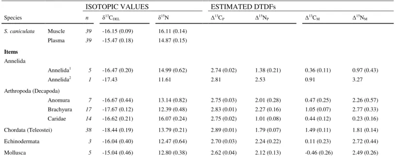
Table 2. Mean isotopic values (±SD) of carbon (δ13CDEL, lipid-extracted) and nitrogen (δ15N) of Scyliorhinus canicula (muscle and
665
plasma) and these prey items from the North Sea and estimated diet-item specific diet tissue discrimination factors (DTDF) for the 666
isotopic model. Prey items were chosen by their presence in collected stomach contents or identified from the literature for this 667
species. Species-specific DTDFs (∆: P = Plasma and M = Muscle) were generated from ∆-diet isotope relationships generated from 668
experimental data (see Fig 3) and were used in the isotopic mixing model SIAR. 669
670
ISOTOPIC VALUES ESTIMATED DTDFs
Species n δ13C DEL δ15N ∆13CP ∆15NP ∆13CM ∆15NM S. caniculata Muscle 39 -16.15 (0.09) 16.11 (0.14) Plasma 39 -15.47 (0.18) 14.87 (0.15) Items Annelida Annelida1 5 -16.47 (0.20) 14.99 (0.62) 2.74 (0.02) 1.38 (0.21) 0.36 (0.11) 0.97 (0.43) Annelida2 1 -17.43 11.61 2.81 2.53 0.91 3.27 Arthropoda (Decapoda) Anomura 7 -16.67 (0.44) 13.14 (0.82) 2.75 (0.03) 2.01 (0.28) 0.47 (0.25) 2.26 (0.57) Brachyura 17 -17.67 (0.12) 12.39 (0.48) 2.83 (0.01) 2.27 (0.16) 1.05 (0.07) 2.77 (0.33) Caridae 14 -16.62 (0.21) 16.07 (0.24) 2.75 (0.02) 1.01 (0.08) 0.44 (0.12) 0.23 (0.16) Chordata (Teleostei) 38 -18.44 (0.19) 13.79 (0.21) 2.89 (0.01) 1.79 (0.07) 1.49 (0.11) 1.81 (0.14) Echinodermata 3 -16.04 (0.40) 12.47 (0.64) 2.70 (0.03) 2.24 (0.22) 0.11 (0.23) 2.72 (0.44) Mollusca 5 -15.04 (0.46) 12.80 (0.38) 2.62 (0.04) 2.12 (0.13) -0.46 (0.26) 2.49 (0.26)
FIGURE LEGENDS
671
Figure 1. (A) Map of the North Sea, where the annual French International Bottom Trawl Survey 672
of 2008 (1-20 February) was conducted using randomized trawl hauls. One haul was randomly 673
performed in each rectangle; the trawl hauls are represented with white circles. (B) Locations 674
where Scyliorhinus canicula were collected, the number next to the black circles is the total 675
number of individuals caught and the “exponent” indicates the number of samples analysed (n = 676
39). 677
Figure 2. Nitrogen and carbon isotopic values (mean ± SD) of plasma and red blood cells (RBC) 678
of Scyliorhinus stellaris for the different diet treatments: (i) S120M120 = switch from smelt (S) to
679
mussel (M) diet at 120 days (Diet Shift. DS); (ii) M120S120 = switched from M to S diet at 120
680
days; (iii) M240 and S240 = remained on the same diet (M or S) for 240 days. The diet treatments
681
M120 and S120 represent the first part of the experiment (0-120 days), before the diet shift occurred
682
(DS). 683
Figure 3. Randomized cumulative prey curve for Scyliorhinus canicula. Mean values of 10 684
randomizations are presented ± SE. 685
Figure 4. Proportional contribution of different potential prey to the diets of Scyliorhinus 686
canicula based on plasma and muscle isotopes (SIAR model) and stomach contents (NI: 687
mean±SD). Boxplots (x-axis) show the distribution of possible contributions from each prey 688
source to the diet of S. canicula that result from the application of the SIAR isotopic model. 689
Values shown are the 25, 75 and 95%, credibility internals respectively for these distributions. 690
Abbreviations for S. canicula prey group are as follows: AN1 Annelida group 1; AN2 Annelida 691
group 2; ANO Anomura; BRA Brachyura; CAR Caridae; TEL Teleostei; ECH Echinodermata; 692
and MOL Mollusca. 693
Figure 5. Relationship between the mean values of (A) nitrogen isotopic ratios (δ15N) and diet 694
tissue discrimination factors (∆15N) and (B) carbon isotopic ratios (δ13C) and diet tissue 695
discrimination factors (∆13C) for the different tissues sampled (black = muscle and white = 696
plasma) for laboratory derived DTDFs. The number at the top of each point identifies the shark 697
study (1 = this study, 2 = Kim et al. 2012a. 3 = Hussey et al. 2010b, and 4 = Kim et al. 2012b). 698
Equations, regression coefficients, and fits are shown for the significant models. 699
Figure 6. Mean proportional contribution of different potential prey to the diets of Scyliorhinus 700
canicula based on plasma and muscle isotopes (SIAR model) with Fixed Discrimination Factors
701
(FDF, ∆13C = 1‰ and ∆15N = 3.2‰) and Diet Tissues Discrimination Factors estimated by 702
regressions (DTDF, Fig 4). Abbreviations for S. canicula prey group are as follows: AN1 703
Annelida group 1; AN2 Annelida group 2; ANO Anomura; BRA Brachyura; CAR Caridae; TEL 704
Teleostei; ECH Echinodermata; and MOL Mollusca. 705
Figure 1. 706 707 552 5314 630 160 20 150 103 10 33 43 11 3313 Scyliorhinus canicula
B
A
Haul
North Sea 552 5314 630 160 20 150 103 10 33 43 11 3313 Scyliorhinus caniculaB
A
Haul
North SeaFigure 2. 708 709 -20 -19 -18 -17 -16 -15 -14 -13 12 13 14 15 16 17 18 19 0 50 100 150 200 250 0 50 100 150 200 250 PLASMA RBC DS DS