Abstract—This paper addresses the problem of changing the operating point of a power system in order to keep voltage security margins with respect to contingencies above some minimal value. Margins take on the form of maximum pre-contingency power transfers either between a generation and a load area or between two generation areas. They are determined by means of a fast time-domain method. We will first discuss the use of a general op-timal power flow, in which linear voltage security constraints are added. The simultaneous control of several (possibly conflicting) contingencies is considered. Then, we will focus on the minimal control change objective. Among the possible controls, emphasis is put on generation rescheduling and load curtailment. Examples are presented on an 80-bus test system as well as on a real system. Index Terms—Dynamic security analysis, generation resche-duling, load curtailment, preventive control, voltage stability.
I. INTRODUCTION
V
OLTAGE stability is a major aspect of power system se-curity analysis in both operational planning and real-time [1], [2]. Voltage security analysis has become even more im-portant in the open-access environment that prevails in an in-creasing number of power systems. In this context, it is the role of the transmission system operator to check security before a set of transactions is accepted, and to take preventive actions as soon as the security margins are deemed insufficient.This paper is devoted to the determination of the best control actions to restore security margins with respect to credible con-tingencies.
Among the available controls, actions on voltages—through transformer ratios, generator voltages, and reactive power injec-tions—are limited by the range of variation allowed for these variables as well as by the risk of pre-contingency overvoltages. On the other hand, active power generation rescheduling and load curtailment can have a significant impact on voltage sta-bility. However, these actions have a cost and hence must be taken in a transparent and optimal manner.
Several publications deal with optimization techniques for preventive control of voltage stability. The various formulations aim at either maximizing a load power margin [5]–[8] or min-imizing an objective function with voltage security constraints [8]–[11]. The approach used in this paper belongs to the second category.
There are basically two approaches to the computation of controls aimed at increasing a security margin.
1) The first approach is to perform a single optimiza-tion providing both the improved margin and the cor-Manuscript received June 6, 2001; revised October 18, 2001.
The authors are with the Department of Electrical Engineering and Com-puter Science (Montefiore Institute), University of Liège, B-4000 Liège, Bel-gium (e-mail: [email protected]).
Publisher Item Identifier S 0885-8950(02)03821-X.
responding controls. Control and dependent variables are handled together. This optimization is performed with at least a set of equality constraints describing system operation at the limit point [5]–[7]. Inequality constraints can be added on the limit point [7] or on both the limit and the base case operating points [8], [11], which requires to incorporate the equality con-straints relative to base case system operation. 2) The second approach is to import into an optimization
of the base case system operation constraints stemming from a separate margin computation and analysis [9], [10].
Although it requires iteration between margin calculation and control adjustments, Approach B is more “open”: e.g., margins can be determined through more accurate, dynamic simulations, while Approach A relies on algebraic (typically load flow) equa-tions treated as equality constraints. In this paper, Approach B is followed, with the fast time-domain quasi-steady-state (QSS) simulation method [2] used to evaluate the system response to contingencies.
To the authors’ knowledge, all publications so far concentrate on a single configuration of the system and, where a contingency is mentioned, the control actions are taken in the post-contin-gency configuration. Our concern is to control the system in the pre-contingency configuration such that security margins are maintained with respect to several (dangerous or potentially dangerous) contingencies simultaneously. In particular, we take into account that controls with positive effects on a contingency may be detrimental to another. Again, Approach B seems more appropriate, in as much as the multiple contingencies can be handled separately (and possibly in parallel), thereby breaking down the problem into more tractable ones.
II. VOLTAGESECURITYMARGINS
Our analysis of voltage security relies upon the definition of a system stress. The latter consists of changes in bus power in-jections which make the system weaker by increasing power transfer over relatively long distances and/or drawing on reac-tive power reserves. Namely, at the th bus, the load acreac-tive power , the load reactive power , or the generator active power
vary according to
where
, , and corresponding base case values; scaling factor;
and participation factors. 0885-8950/02$17.00 © 2002 IEEE
Fig. 1. Binary search of a security margin.
These equations can be written in vector form as
(1) where
vector of bus injections; base case value;
vector defining the “direction of stress.”
Typical stresses consist of increasing load in an area A and gen-eration in a remote area B
or decreasing generation in an area A and increasing generation
in a remote area B .
For a given direction of stress, the margin relative to a con-tingency is the maximum value of such that the system can withstand this contingency [2]. Such a margin refers to pre-con-tingency parameters that operators can either observe or control. The margin relative to a contingency can be determined by the simple and robust binary search. This consists of building a smaller and smaller interval , where corresponds to a stable post-contingency evolution and to an unstable one,
until becomes lower than a tolerance . The search
starts with and , a maximum stress of
in-terest. At each step, the interval is divided in two equal parts; if the midpoint is found stable (respectively, unstable) it is taken as the new lower (respectively, upper) bound. The final value of is the sought margin . The procedure is sketched in Fig. 1, where the dashed arrows show the sequence of tested stress levels. It will be briefly illustrated in Section III-B.
In real-time applications, it is essential to filter out the con-tingencies and quickly identify those having low margins for the stress under concern. To this purpose, contingencies can be simulated on the system stressed at level , using a simpli-fied method such as a post-contingency load flow. Contingen-cies which cause the latter to diverge or some voltages to drop by more than some amount are labeled potentially dangerous and are processed through the binary search using QSS simulation. Among them, the false alarms are discarded at the first step of the search.
Detailed examples and computing times relative to two real systems can be found in [4].
III. LINEARIZEDVOLTAGESECURITYCONSTRAINTS A system is voltage secure when, for a specified direction of stress , the margin relative to any of the specified contin-gencies is larger than some threshold . Preventive voltage se-curity control aims at modifying the pre-contingency operating point so that this constraint is met. In the sequel, we choose the
Fig. 2. Power injection space.
control variables among the injection vector (although the derivation could be extended to other controls as well).
Clearly, an essential information needed for control is the sen-sitivity of the margins to .
A. Derivation of Voltage Security Constraints
A simple, brute force approach consists in approximating the sensitivities by a ratio of finite differences, assuming a small variation and evaluating the resulting margin variation . To guarantee accuracy, the magnitude of must be chosen properly and the margins must be computed with a tolerance smaller than what is needed for security monitoring. This requires to perform more steps in the binary search. On the other hand, each binary search can start from a
narrower interval .
Deriving an accurate analytical expression of the sensitivities is a challenging—if at all solvable—problem. Indeed, we seek to determine how far changes in the pre-contingency operating point influence the maximum stress that can be imposed to the system, such that its response to a contingency is stable. A con-tribution of this paper is to show that the technique used in [12] for post-contingency control provides reasonably accurate in-formation for the sought pre-contingency application.
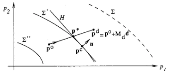
The derivation is obtained as follows [2], [5], [12], [13]. The most common voltage instability mechanism is the loss of a long-term equilibrium. A two-dimensional view of the (pa-rameter) space of power injections is given in Fig. 2.
corre-sponds to the base case demand, while
corre-sponds to the desired margin. Under the effect of a contingency, the feasible region—where the system has a long-term equilib-rium—shrinks, and its boundary changes from to . falls outside the new feasible region, and instability results. For the more severe contingency changing to , the base case point itself falls outside the new feasible region, which means that the system has no margin with respect to this contingency.
Preventive control aims at changing into so that falls within the feasible region.
At this point, we use a linear approximation of the boundary surfaces, i.e., in Fig. 2 we approximate by its tangent hyper-plane . The latter is identified from the “critical point” and the normal vector , whose computation will be explained in
the sequel. In order to be brought back on the
feasible side of , must satisfy
Introducing this result in (2) yields
(3) The row vector premultiplying is the sensitivity of the margin to and (3) expresses that the linear approximation of the post-control margin should be larger than .
Denoting the set of long-term equilibrium equations by (4) where is the state vector; the normal vector is given by
(5) in which is the Jacobian of with respect to and is the left eigenvector relative to the zero eigenvalue of the Jacobian
on the bifurcation surface [2], [13].
Note that is computed at a point where some generators may have switched under field current limit while they control their voltages in the base case. The voltage set points of such generators cannot be taken as control variables, since they do no longer appear in the final set of equations.
B. Illustrative Example
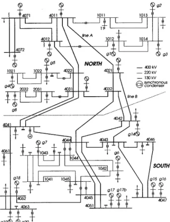
We consider the 80-bus system shown in Fig. 3, a variant of the “Nordic 32” system used, for example, by CIGRE Task Force 32.02.08 on long-term dynamics (1995). A rather heavy power transfer takes place from “north” to “south” areas.
The QSS long-term simulation reproduces the dynamics of load tap changers and overexcitation limiters. Note that there is no slack-bus in the QSS model; instead, generators respond to a disturbance according to governor effects [2]. Moreover, it is assumed that only the generators of the north area participate to frequency control (i.e., the others have infinite speed droops).
The stress of concern is a load increase in the south area MW/180 MVAr ) covered by a generation
in-crease in the north area ( MW, accounting for
losses), each according to participation factors.
We consider a set of 49 contingencies, out of which 20 have a
margin lower than . Taking MW, five QSS
simula-tions are needed to find a limit. The left plot in Fig. 4 shows the time evolution of a 400-kV bus voltage, under the effect of a con-tingency applied at s. The curves relate to
and respectively.
For each contingency of interest, the instability mode is iden-tified from the marginally unstable case, using the technique de-tailed in [2] and [12]. First, the critical point is identified using the sensitivities of the total reactive generation to each reactive load. The time evolution of such a sensitivity is shown in the right plot of Fig. 4, relative to the marginally unstable case. The
Fig. 3. Slightly modified “Nordic 32” test system.
Fig. 4. Time evolution of a bus voltage and a@Q =@Q sensitivity.
critical point is crossed at s, where sensitivities change sign “going through infinity.” At this point, the simultaneous it-eration method applied to the Jacobian provides a small real positive dominant eigenvalue and the corresponding left eigen-vector to be substituted in (5).
Under the effect of field current limiters, the dominant (real) eigenvalue may “jump” from a negative to a positive value (e.g., [2, pp. 255–260]), instead of smoothly passing through zero. The above sensitivities correspondingly switch from positive to negative without assuming very large values, as in Fig. 4. As reported in [12], in all practical cases, we found it satisfactory to compute at the first point where negative sensitivities are observed.
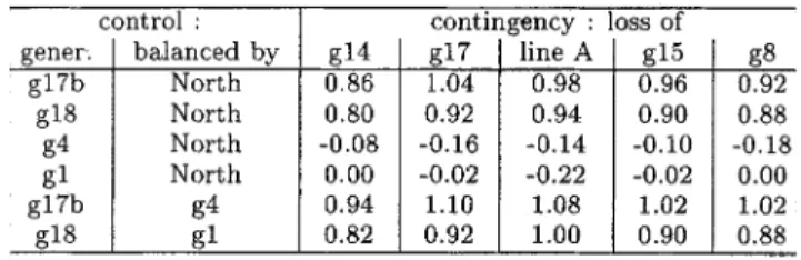
Table I shows the sensitivities of margins to controls given by (3), for the five most severe contingencies and for different controls. The sensitivity to an active generation is the margin increase for a small increase on this generation, balanced by a decrease of northern generations, as dictated by frequency con-trol. Such values are presented in the first four rows of Table I. The last two rows, on the other hand, correspond to a shift of
TABLE I
NORDIC32 SYSTEM: SENSITIVITIESGIVEN BY(3)
TABLE II
SAMESYSTEM: SENSITIVITIESOBTAINED BYFINITEDIFFERENCES
power from one generator to another. The values have been ob-tained by subtracting the corresponding sensitivities.
Expectedly, these results show that margins are increased mainly by north to south power shifts, and much less by internal shifts within the north area.
For comparison purposes, Table II shows the same sensitiv-ities obtained by finite differences. For each generator of con-cern, a 50-MW production increase has been considered, com-pensated according to governor effects. All margins have been computed with a tolerance of 2 MW for the sake of accuracy. Numerical discrepancies are to be expected considering that a finite difference is used, tap changers deadband make the QSS simulation somewhat insensitive, etc. Nevertheless, there is a good general agreement between both approaches. In particular, the ranking of control actions is the same by both approaches.
IV. OPTIMIZATIONAPPROACHES
Assume that system operation in the base case is character-ized by margins smaller than the desired value . The corresponding contingencies will be labeled as “harmful,” the remaining ones being “harmless.” We seek to modify so that the margins become at least as large as . For each of them, (3) can be rewritten as
(6)
A. Control Provided by an Optimal Power Flow (OPF)
The inequalities (6) can be incorporated to the constraints of an OPF aimed at determining the -dimensional vector in some optimal manner.
In principle, this OPF can incorporate any other constraint, in particular, thermal limits relative to the base case and post-con-tingency configurations, thereby offering an integrated control of thermal and voltage problems.
Various OPF objectives can be considered. In a real-time en-vironment, the insufficient margins represent transmission
con-gestions, which should be corrected by adjusting the market-based generation scheme. Decomposing each correction into
with , , a simple
objec-tive is
(7)
where, for a generator which can be rescheduled, (respec-tively, ) is the incremental (respectively, decremental) bid-ding price, and for a load which can be curtailed,
while is the curtailment price.
Let be the new margins
ob-tained after modifying according to the OPF. We expect to
have with (at least) one
in-equality constraint (6) binding at the solution, i.e.,
or, in practice, , where
is a tolerance. This corresponds to the most dangerous contin-gency in the post-control situation, with a margin just equal to
.
Two situations, however, may prevent us from reaching this objective in a single step, as discussed hereafter.
1) Under- or over-correction of margins. We have empha-sized that the inequalities (6) are somewhat approximate with respect to the true nonlinear constraints. As a conse-quence, it can happen that some margins are still smaller than or, on the contrary, all of them are significantly larger than . In such cases, we compute improved sen-sitivities and redetermine the OPF correction to apply to
(not ). Now, we only have new margins to
improve sensitivities. To face this lack of infor-mation, we correct all the sensitivities
relative to the th contingency by the scaling factor (8)
in which the numerator represents the real change in the th margin and the denominator the one expected from linearization. This approximation is justified by the ob-servation that, for a given contingency, the relative values of the various sensitivities are correct. In principle, the procedure has to be repeated until the margins are dis-tributed as indicated previously.
2) Antagonistic controls. It can happen that changing to meet the harmful contingency inequality constraints (6) causes harmless contingencies to become harmful. A first solution consists of extending the set of inequali-ties (6) to contingencies having a margin in an interval
, where we assume that margins larger than (i.e., much larger than ) will not fall below . Note that incorporating to the OPF more inequalities (6) than necessary has no consequence; the latter will merely re-main nonbinding. Alternatively, we may stick with the threshold and, if some new margins fall below , add the corresponding inequalities to the former set and perform a new OPF.
from a very unstable trajectory may be more delicate than from a marginally unstable one.
B. Minimal Control Change: A Simplified Formulation
In the sequel, we focus on determining the minimal rescheduling and/or load curtailment needed to restore a certain level of voltage security. This is a particular case of the objective (7), corresponding to , i.e., to
(9)
We ignore constraints on the pre-contingency operating point, and restrict our set of inequality constraints to
(10)
(11) Finally, we neglect the variations of network active losses and use instead the simple power balance equation
(12)
If this is not deemed acceptable, a full OPF incorporating (10) and (11) can be used (in which losses are taken into account through load flow equality constraints).
The above -norm objective tends to put the control effort on generators with the highest sensitivities, even if the gap with respect to other generators is small. This drawback can be at-tenuated by limiting the amplitude of the control changes. An alternative is to use the -norm objective
(13)
The latter generally leads to a large number of injection changes, which can be impractical for transmission system operators. This disadvantage could be mitigated by performing a second optimization, after removing from the candidate controls, gen-erators with small contributions .
The above optimization problems can be solved using stan-dard linear or quadratic programming software.
In the above formulation, controls are of active power nature, but reactive aspects can be accounted for in the computation of the sensitivities . More precisely, if a change in active power
at the -bus is accompanied by a change
Fig. 5. Overall flowchart of the computational procedure.
of the corresponding reactive power injection, the effective sen-sitivity is taken as
(14) This formula is applied in the following two cases.
Load curtailment. When load is cut, both active and
reac-tive powers vary. In the absence of a more precise informa-tion, loads can be decreased under constant power factor,
in which case .
Generation rescheduling. It is well known from the
capa-bility curves that increasing the active production of a gen-erator decreases its reactive reserve. To account for this ef-fect, is taken as the (negative) slope of the curve. This applies only to generators under reactive power limit at the critical point where is computed.
If the last term in (14) is large enough, when decreasing active power generation, the benefit of an increased reactive reserve may outweight the detrimental effect of importing active power from remote generators.
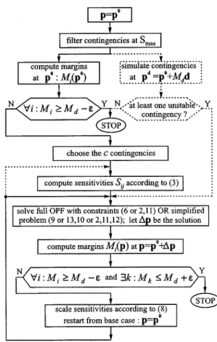
The whole computational procedure is sketched in Fig. 5, where the dashed lines correspond to the variant mentioned in the last paragraph of Section IV-A.
C. Illustrative Example
We proceed with the example of Section III-B. For the same
TABLE III
NORDIC32 SYSTEM: MARGINSBEFORE ANDAFTERCONTROL
TABLE IV
NORDIC32 SYSTEM: CHANGES INGENERATION ORLOAD(INMEGAWATTS)
are harmful, i.e., have a margin smaller than , as shown in the second column of Table III. To anticipate for antagonistic
effects, we choose MW. This leads to monitoring
contingencies.
We consider hereafter four combinations of controls and ob-jectives, whose results are detailed in Tables III and IV.
Case A: norm, generation rescheduling. The
optimiza-tion problem (9)–(11) leads to reschedule 178 MW
(ob-jective function (9) MW). It consists of
increasing the production of generators g7 and g17b which are located in the voltage sensitive area, while decreasing the generation of g4, located far away in the north. This de-creases the north to south power transfer. Since after this generation shift, all margins are above 300 MW and one of them (loss of g14) approaches this threshold by less than MW, there is no need for another optimization. We observe that the margin relative to the loss of gener-ator g17b increases significantly less (57 MW) than the others (from 158 to 186 MW). This is due to the fact that rescheduling increases the production of g17b by 135 MW, and hence the loss of this increased generation causes the north to south transfer to increase correspondingly (due to already mentioned governor effects).
Case B: norm, load curtailment. In this second
ex-ample, both generation rescheduling and load curtailment
Fig. 6. Overall structure of the Hydro-Québec 735-kV system.
are allowed to restore security margins. The maximal inter-ruptible fraction of each load is limited to 20% and power factors are preserved. The solution consists of shedding 147 MW in the voltage sensitive area, and again compen-sating on the remote generator g4. With respect to Case A, the objective function (9) reaches a lower value (294 MW) thanks to the larger number of controls offered. In this case, a second optimization is needed to make the smallest margin approach 300 MW by less than .
Case C: norm, generation rescheduling. This case is the
same as Case A, except for the objective, which is taken as (13). This yields a larger number of changes, each of smaller magnitude. The changes have been, however, lim-ited to 11 generators, selected on the basis of their sensi-tivities. The total rescheduling is 187 MW, i.e., somewhat more than that with the norm.
Case D: norm, load curtailment. Similarly, the effort is
shared by a larger number of loads than in Case B. As a general remark, the optimization yields a smaller number of changes and a smaller total power change. On the other hand, the optimization is more robust with respect to inaccuracies on the sensitivities that could lead to shifting the control effort from one generator to another.
D. Example From the Hydro-Québec System
We briefly present here an example of antagonistic controls observed on the Hydro-Québec (HQ) system. Fig. 6 sketches the structure of the 735-kV transmission system. More details can be found in [4]. Let us only emphasize here that the system response is much influenced by the operation of an extended set of shunt reactor tripping devices. The long-term evolution of voltages is thus very dynamic by nature, which has motivated the adoption of QSS simulation by HQ engineers for security limit computations. Examples of the latter are given in [4].
The stress consists of increasing the demand in the Mon-treal-Québec (MQ) area, where most of the load is concen-trated, and the generation in the JB, CF, and MO areas. Security limits are computed for a set of 37 contingencies, with
MW. Two contingencies have limits lower than (see Table V). They are located in the MO–MQ and JB–MQ corri-dors, respectively.
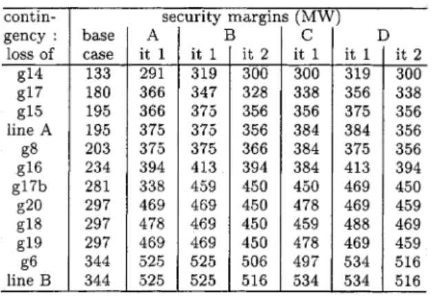
We consider the minimal generation rescheduling in the sense, corresponding to four values of . The computed con-trols are shown in Table VI. Three successive optimizations are required on the average. This is attributed to the fact that margins change more abruptly with controls, under the effect of shunt re-actor trippings.
TABLE VI
HYDRO-QUÉBECSYSTEM: GENERATIONRESCHEDULING(INMEGAWATTS)
For MW, contingency 6 is harmful. Expectedly,
the minimal generation rescheduling consists of decreasing the power flow in the MO–MQ corridor, shifting 35 MW from g9241 (MO area) to g7 and g17 (MQ area). Both margins are increased. However, after this preventive control, almost no active power reserve is left to the MQ area. Therefore, when is set to 400 MW, the minimal generation rescheduling slightly increases the production of g49, located in the JB area. This is accompanied by a slight decrease in the margin of contingency 19 (which, however, remains above ). If is set to 525 MW, for instance, the problem is infeasible. Indeed, at this level, bringing both margins above would require to decrease both corridor flows. The largest value of for which a solution exists is 425 MW. The corresponding results are given in Tables V and VI; both margins have been raised at the 425 MW threshold. By setting (for checking purposes) to 525 MW for contingency 6 and 400 MW for contingency 19, the problem is feasible again, with the solution shown in the last column of each table.
V. CONCLUSION
This paper has dealt with the preventive control to restore margins at a desired level. Emphasis has been put on power injections as control variables.
Among the features of the proposed method, let us quote: • the determination of sensitivities of pre-contingency
mar-gins to controls using post-contingency information; • the derivation of linearized security constraints to be
in-cluded in an OPF, possibly together with the similar con-straints stemming from line overloads in a unified treat-ment of voltage and thermal security;
• a technique to compensate for the linear approximation (two OPF runs are generally sufficient to make the system secure without under- or over-correcting);
• the simultaneous control of all harmful contingencies; • the handling of antagonistic controls by incorporating
some harmless contingencies in the constraints.
Successful results have already been obtained when extending the techniques described in this paper to the mod-ification of bilateral transactions (stemming, for instance,
are now available to determine such margins [4]. Their coupling with appropriate filtering techniques and their implementation on modern (possibly distributed) computer hardware allow to envisage real-time applications.
REFERENCES
[1] C. W. Taylor, “EPRI power system engineering series,” in Power System
Voltage Stability. New York: McGraw-Hill, 1994.
[2] T. Van Cutsem and C. Vournas, Voltage Stability of Electric Power
Sys-tems. Norwell, MA: Kluwer, 1998.
[3] T. Van Cutsem, “Voltage instability: Phenomena, countermeasures, and analysis methods,” Proc. IEEE, vol. 88, pp. 208–227, 2000.
[4] T. Van Cutsem, F. Capitanescu, C. Moors, D. Lefebvre, and V. Ser-manson, “An advanced tool for preventive voltage security assessment,” in Proc. VII SEPOPE Conf., Curitiba, Brazil, 2000, Paper IP-035. [5] I. Dobson and L. Lu, “Computing an optimum direction in control space
to avoid saddle node bifurcation and voltage collapse in electric power systems,” IEEE Trans. Automat. Contr., vol. 37, pp. 1616–1620, Oct. 1998.
[6] C. A. Canizares, “Calculating optimal system parameters to maximize the distance to saddle-node bifurcations,” IEEE Trans. Circuits Syst. I, vol. 45, pp. 225–237, 1998.
[7] R. Wang and R. H. Lasseter, “Re-dispatching generation to increase power system security margin and support low voltage bus,” IEEE Trans.
Power Syst., vol. 15, pp. 496–501, May 2000.
[8] W. Rosehart, C. A. Canizares, and V. H. Quintana, “Optimal power flow incorporating voltage collapse constraints,” in Proc. IEEE PES Summer
Meeting, Edmonton, Canada, 1999, pp. 820–825.
[9] X. Wang, G. C. Ejebe, J. Tong, and J. G. Waight, “Preventive/corrective control for voltage stability using direct interior point method,” IEEE
Trans. Power Syst., vol. 13, pp. 878–883, Aug. 1998.
[10] Z. Feng, V. Ajjarapu, and D. J. Maratukulam, “A comprehensive ap-proach for preventive and corrective control to mitigate voltage col-lapse,” IEEE Trans. Power Syst., vol. 15, pp. 791–797, May 2000. [11] E. Vaahedi, Y. Mansour, C. Fuchs, S. Granville, M. de Lujan Lastore,
and H. Hamadanizadeh, “Dynamic security constrained optimal power flow/VaR planning,” IEEE Trans. Power Syst., vol. 16, pp. 38–43, Feb. 2001.
[12] C. Moors and T. Van Cutsem, “Determination of optimal load shedding against voltage instability,” in Proc. 13th PSCC, Trondheim, Norway, 1999, pp. 993–1000.
[13] S. Greene, I. Dobson, and F. L. Alvarado, “Sensitivity of the loading margin to voltage collapse with respect to arbitrary parameters,” IEEE
Trans. Power Syst., vol. 12, pp. 262– 272, Feb. 1997.
Florin Capitanescu received the B.S. and M.Sc. degrees in electrical power
en-gineering from the University “Politehnica” of Bucharest, Bucharest, Romania, in 1997 and 1998, respectively, and the DEA degree from the University of Liège, Liège, Belgium, in 2000, where he is currently pursuing the Ph.D. de-gree in preventive aspects of voltage security.
Thierry Van Cutsem (M’94) received the electrical-mechanical engineering
and the Ph.D. degrees from the University of Liège, Liège, Belgium, in 1979 and 1984, respectively.
Since 1980, he has been with the Belgian National Fund for Scientific Re-search (FNRS) of which he is now a ReRe-search Director. He is currently an Ad-junct Professor at the University of Liège. His research interests are in power system dynamics, control and stability, numerical simulation, and security anal-ysis, in particular, voltage stability and security.