HAL Id: hal-01407514
https://hal.inria.fr/hal-01407514
Submitted on 2 Dec 2016
HAL is a multi-disciplinary open access
archive for the deposit and dissemination of
sci-entific research documents, whether they are
pub-lished or not. The documents may come from
teaching and research institutions in France or
abroad, or from public or private research centers.
L’archive ouverte pluridisciplinaire HAL, est
destinée au dépôt et à la diffusion de documents
scientifiques de niveau recherche, publiés ou non,
émanant des établissements d’enseignement et de
recherche français ou étrangers, des laboratoires
publics ou privés.
Nearest Neighbors Graph Construction: Peer Sampling
to the Rescue
Yahya Benkaouz, Mohammed Erradi, Anne-Marie Kermarrec
To cite this version:
Yahya Benkaouz, Mohammed Erradi, Anne-Marie Kermarrec. Nearest Neighbors Graph Construction:
Peer Sampling to the Rescue. 4th International Conference, NETYS 2016, Marrakech, Morocco, May
18-20, 2016, Revised Selected Papers, May 2016, Marrakech, Morocco. pp.48 - 62,
�10.1007/978-3-319-46140-3_4�. �hal-01407514�
Peer Sampling to the rescue
Yahya Benkaouz1, Mohammed Erradi1, and Anne-Marie Kermarrec2
1 Networking and Distributed Systems Research Group
ENSIAS, Mohammed V University Rabat, Morocco
[email protected],[email protected]
2 INRIA Rennes
France
Abstract. In this paper, we propose an efficient KNN service, called KPS (KNN-Peer-Sampling). The KPS service can be used in various contexts e.g. recommendation systems, information retrieval and data mining. KPS borrows concepts from P2P gossip-based clustering proto-cols to provide a localized and efficient KNN computation in large-scale systems. KPS is a sampling-based iterative approach, combining ran-domness, to provide serendipity and avoid local minimum, and cluster-ing, to ensure fast convergence. We compare KPS against the state of the art KNN centralized computation algorithm NNDescent, on multiple datasets. The experiments confirm the efficiency of KPS over NNDescent: KPS improves significantly on the computational cost while converging quickly to a close to optimal KNN graph. For instance, the cost, ex-pressed in number of pairwise similarity computations, is reduced by ≈ 23% and ≈ 49% to construct high quality KNN graphs for Jester and MovieLens datasets, respectively. In addition, the randomized nature of KPS ensures eventual convergence, not always achieved with NNDescent. Keywords: K-Nearest Neighbors, Clustering, Sampling, Randomness.
1
Introduction
Methods based on nearest neighbors are acknowledged as a basic building block for a wide variety of applications [12]. In an n object system, a K-nearest-neighbors (KNN) service provides each object with its k most similar objects, according to a given similarity metric. This builds a KNN graph where there is an edge between each object and its k most similar objects. Such a graph can be leveraged in the context of many applications such as similarity search [5], machine learning [15], data mining [22] and image processing [8]. For instance, KNN computation is crucial in collaborative filtering based systems, providing users with items matching their interests (e.g Amazon or Netflix). For instance, in a user-based collaborative filtering approach, the KNN provides each user
with her closest ones, i.e. the users which have the most interests in common. This neighborhood is leveraged by the recommendation system to provide users with items of interest, e.g. the most popular items among the KNN users.
The most straightforward way to construct the KNN graph is to rely on a brute-force solution computing the similarity between each pair of nodes (in the rest of this paper, we call a node an element of the system and the KNN graph. A node can refer to an object or a user for instance). Obviously the high complexity of such an approach, O(n2) in a n node system, makes this solution
usable only for small datasets. This is clearly incompatible with the current Big Data nature of most applications [4]. For instance, social networks generate a massive amount of data (e.g on Facebook, 510,000 comments, 293,000 status updates and 136,000 photo uploads are generated every minute). Processing such a huge amount of data to extract meaningful information is simply impossible if an approach were to exhaustively compute the similarity between every pair of nodes in the system. While traditional clustering approaches make use of offline generated KNN graphs [15, 20], they are not applicable in highly dynamic settings where the clusters may evolve rapidly over time and the applications relying on the KNN graph expect low latencies. Hence, a periodic recomputation of the KNN graph is mandatory. The main challenge when applying KNN to very large datasets is to drastically reduce the computational cost.
In this paper, we address this challenge by proposing a novel KNN com-putation algorithm, inspired from fully decentralized (peer-to-peer) clustering systems. More specifically, peer-to-peer systems are characterized by the fact that no peer has the global knowledge of the entire system. Instead, each peer relies on local knowledge of the system, and performs computations using this restricted sample of the system. Yet the aggregated operations of all peers make the system converge towards a global objective. In this paper, we present KPS (KNN-Peer-Sampling), a novel sampling-based service for KNN graph construc-tion that combines randomness to provide serendipity and avoid local minimum, and clustering to speed up the convergence therefore reducing the overall cost of the approach. Instead of computing the similarity between a node and all other nodes, our approach relies on narrowing down the number of candidates with which each node should be compared. While a sampling approach has also been proposed in NNDescent [13], acknowledged as one of the most efficient so-lutions to the KNN problem currently, we show in our experiments that KPS achieves similar results with respect to the quality of the KNN graph while dras-tically reducing the cost. In addition, KPS avoids the local minimum situation of NNDescent and ensures that the system eventually converges.
To summarize, the contributions of this paper are: (i) the design of a novel, scalable KNN graph construction service that relies on sampling, randomness and localized information to quickly achieve, at low cost, a topology close to the ideal one and eventually ensures convergence. Although we focus on a centralized implementation of KPS, it can also be implemented on a decentralized or hybrid architecture, precisely due to its local nature; and (ii) an extensive evaluation of KPS and a comparison with the state of the art KNN graph construction
algorithm NNDescent, on five real datasets. The results show that KPS provides a low-cost alternative to NNDescent.
The remainder of this paper is structured as follows: Section 2 presents the suggested KPS. Section 3 describes the experimental setup. Section 4 discusses the results. Section 5 presents related works. Finally, Section 6 presents conclu-sions and expected future work.
2
The KNN Peer Sampling Service
KPS is a novel service that starting from a random graph topology, iteratively converges to a topology where each node is connected to its k nearest neighbors in the system. The scalability of KPS relies on the fact that instead of computing the similarity of a node with every other node in the system, only local informa-tion is considered at each iterainforma-tion. This sample, referred as the candidate set, is based only on the neighborhood information available in the KNN graph. This significantly reduces the number of similarity computations needed to achieve the KNN topology.
We consider a set D of n nodes (|D| = n). Each node p is associated with a profile. A profile is a structured representation of a node p, containing multi-ple features that characterize a node. For instance, in user-based collaborative filtering recommendation systems, a node represents a user u. The user profile in this context is typically a vector of preferences gathering the ratings assigned by the user u to different items (movies, books). In an item-based system, the item profile is generally the feature vector that represents the item, or a vector containing a list of users who liked that item for instance.
We also consider a sampling function sample(D, k), that, given a set of nodes in D, and k ∈ N, returns a subset of k nodes selected uniformly at random from D. We assume a function similarity(pi, pj) that computes the similarity between
two nodes, i.e. the similarity between two profiles pi and pj. The similarity can
be computed using several metrics (e.g. Jaccard, cosine, etc). KPS is generic and can be applied with any similarity metric.
Let αp be the number of updates in a given iteration for a node p. In other
words, αp reflects the number of changes that happen in the neighborhood of p
over the last iteration. Somehow αpcaptures the number of potential new
oppor-tunities provided to p to discover new neighbors. KPS constructs the candidate set such that: The candidate set of p contains the neighbors of p, the neighbors of αp neighbors and k − αp random nodes. Those αp neighbors are randomly
selected including new and old neighbors. This operation limits the size of the candidate set. KPS does not explore all the nodes two hops away since that can represent a large fraction of the network. This is particularly true for high degree nodes. Instead, KPS limits the exploration to a subset of neighbors. The reason why KPS considers the direct neighbors to be added to the candidate set is to account for potential dynamics. This makes KPS able to dynamically update the KNN graph as nodes profiles change over time.
Algorithm 1 The KPS Service Algorithm 01. For each p ∈ D do 02. KN Np= sample(D, k) 03. αp= k 04. End for 05. Do 06. For each p ∈ D do 07. oldN Np= KN Np 08. candidateSetp.add(KN Np)
09. selectedN eighborsp= sample(KN Np, αp)
10. For each q ∈ selectedN eighborsp do
11. candidateSetp.add(KN Nq)
12. End for
13. candidateSetp.add(sample(D, k − αp))
14. For each n ∈ candidateSetp do
15. score[n] = similarity(P rof ilen, P rof ilep)
16. End for 17. KN Np= subList(k, sort(score)) 18. αp= k − sizeOf (OldN Np∩ KN Np) 19. End for 20. WhileP pαp> 0
Algorithm 1 represents the pseudocode of the algorithm used in the KPS service. Initially, each node p starts with a random set of neighbors. This forms the initial KNN graph (line 02). Therefore, the initial value of αp is k (line 03).
At each iteration, the candidate set of each node includes its current neighbors (line 08), the neighbors of αp neighbors (lines 09 - 12) and k − αp random
neighbors (line 13).The k − αp nodes are randomly selected from the whole set
of the system nodes. So, they might contain already-candidate nodes. Finally, the KNN of each node is updated, by selecting the k closest neighbors out of its candidate set (lines 14 - 17). At each iteration, the value of αp is re-computed,
for each node, based on the number of changes in the node’s neighborhood (line 18).
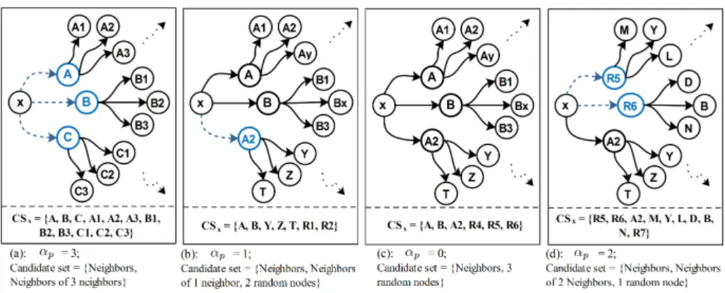
We illustrate several scenarios of KPS operations in figure 1. Based on the value of the parameter αp (number of updates in the KNN list of the node
x), the composition of the candidate set of this node can take several forms. In this scenario, we run the KPS protocol for k = 3. Therefore, αp takes values
between 0 and 3. In the first iteration (Fig. 1a), the neighbors of x are (KN Nx=
{A, B, C}). As the links in the first KNN graph are randomly built, nodes in the set KN Nxare considered as newly discovered nodes, thus αp= k = 3. The
current neighbors present an opportunity to discover relevant new neighbors and considering random nodes is unnecessary. Therefore, the candidate set of x will contain all neighbors and their neighbors. Assuming that, in the second iteration, only the node A2 was added to the KN Nx. Thus, αp= 1 (Fig. 1b). In this case,
Fig. 1: Example scenarios of the KPS service algorithm for k = 3. (The black arrows represent old links and the blue dashed ones are new links)
the candidate set contains, the list of neighbors, the neighbors of αp neighbors
and (k − αp) random nodes. Assuming that, in the third iteration (Fig. 1c), the
KNN list of x remains unchanged KN Nx= {A, B, A2}. This means that αp= 0.
In this case, only random nodes are considered in the candidate set. This might result in the appearance of nodes with higher similarities such as the random nodes R5 and R6 (Fig. 1d).
3
Experimental Setup
In this section, we describe the experimental setup that we rely on to evaluate the efficiency of KPS. More specifically, we describe the competitor, NNDescent [13], that we compare KPS against. We also describe the datasets that we used in the evaluation as well as the evaluation metrics.
3.1 NNDescent Algorithm
NNDescent [13] is a recent KNN algorithm which is acknowledged as one of the best generic KNN centralized approach. Similarly to KPS and previous gossip-based protocols [6, 7, 18, 24], NNDescent relies on two principles: (i) the assump-tion that “The neighbor of a neighbor is also likely to be a neighbor” and (ii) a reduced candidate set to limit the number of similarity computations at each iteration.
The basic algorithm of NNDescent starts by picking a random approximation of KNN for each object, generating a random graph. Then, iteratively, NNDe-scent iterates to improve the KNN topology by comparing each node against its current neighbors’ neighbors, including both KNN and reverse KNN (i.e in and out degree in the graph). KNN terminates when the number of updates in the graph reaches a given threshold, assuming that no further improvement can be made. Thus, in NNDescent, the candidate set of each node contains the
neighbors of neighbors and the reverse neighbors’ neighbors, called RNN. The RNNs are defined in such a way that: Given two nodes p and q, if p ∈ KN Nq
then q ∈ RN Np. Multiple strategies are then proposed to improve the efficiency
of the algorithm:
1. A local join operation takes place on a node. It consists of computing the similarity between each pair p, q ∈ KN N ∪ RN N , and updating both the KNN lists of p and q based on the computed similarity.
2. A boolean flag is attached to each object in the KNN lists, to avoid comput-ing similarities that have been already computed.
3. A sampling method is used in order to limit the size of the reverse KNN. In order to prepare the list of nodes that will participate to the local join operation, NNDescent differentiate old nodes (with a false flag) from new nodes (with a true flag). The sampling method works as follows: Firstly, NNDescent samples ρk out of the KNN, where ρ ∈ (0, 1] is a system param-eter. Then, based on the flag of the sampled nodes, it creates two RNN lists: new’ and old’. After that, two sets s1and s2are created in such a way that:
s1 = old ∪ sample(old0, ρk) and s2 = new ∪ sample(new0, ρk). Finally, the
local join is conducted on elements of s1, and between s1 and s2 elements.
4. An early termination criterion is used to stop the algorithm when further iterations can no longer bring meaningful improvements to the KNN graph. Therefore, the main differences between KPS and NNDescent are the fol-lowing: (i) NNDescent starts from a uniform topology and therefore depending on the initial configuration and the input (dataset), the algorithm might never converge to the ideal KNN graph; (ii) the fact that the candidate set in NNDe-scent contains nodes from RNN and KNN; (iii) the sampling approach used to define the candidate set is different in both approaches; and (iv) KPS adds some random nodes that turn out to be very useful to explore the graph and later to reduce the risk of being stuck in local minimum.
3.2 Datasets Description
We conducted the evaluation of KPS against five real datasets. Figures are sum-marized in Table 1: Shape and Audio also used in [13] as well as MovieLens [3], Jester [2] and Flickr. In the following, we detail how node profiles are built for these datasets:
– The Audio dataset contains features extracted from the DARPA TIMIT col-lection, which contains recordings of 6, 300 English sentences. Each sentence is broken into smaller segments from which the features were extracted. Each segment feature is treated as an individual node.
– The Flickr dataset is constructed based on [17]. This dataset contains 22, 872 image profiles. A Flickr image profile consists of a set of tags associated to the image.
Dataset Object Profile content Nb. Profiles Profile size
Audio Records Audio features 54387 192
Flickr Image Images tags 22872 9 in avg.
Jester User Jokes ratings 14116 100
MovieLens User Movies 6040 165 in avg.
Shape 3D shape model Model features 28775 544
Table 1: Datasets characteristics
– The MovieLens raw data consists of 1, 000, 209 anonymous ratings of ap-proximately 3, 900 movies made by 6, 040 MovieLens users [3]. Based on the collected data we extracted the users’ profiles, such that items in a given user profile contains list of movies that received a rating in the range [3, 5]. – The Jester dataset [1] contains data collected from the Jester Joke Recom-mender System [2]. We selected only profiles of users that rated all jokes. Therefore, the dataset contains 14, 116 user profiles. Each user profile con-tains ratings of a set of 100 jokes.
– The Shape dataset contains about 29, 000 3D shape models. It consists of a mixture of 3D polygonal models gathered from commercial viewpoint mod-els, De Espona Modmod-els, Cacheforce models and from the Web. Each model is represented by a feature vector.
3.3 Similarity Metrics
Depending on the nature of nodes profiles, we rely on different similarity metrics: Jaccard similarity and the cosine similarity. Given two sets of attributes, the Jaccard similarity is defined as the cardinality of the intersection divided by the size of the union of the two sets: J accard(s1, s2) = |ss1∩s2
1∪s2|. The cosine similarity measure is represented using the dot product and the magnitude of two vectors: Cosine(v1, v2) =||vv1.v2
1||.||v2||.
When the node profiles of a given dataset are of different sizes, we use Jaccard similarity, where a node profile is considered as a set. We used the Jaccard similarity metric for MovieLens and Flickr datasets. Otherwise, when the profiles of a dataset are of the same size and when the order of profiles’ attributes is important, we use the cosine similarity. Thus, we used the cosine similarity metric for Jester, Shape and Audio datasets.
3.4 Evaluation Metrics
To measure the accuracy of KPS, we consider the recall of the KNN lists. This metric tells us to what extent the KNN lists match the ideal ones. The recall for a given node is computed using the following formula: R = T P/(T P + F N ), such that: T P (True Positive) is the number of nodes belonging to the nearest neighbors that truly belong to the node’s KNN; F N (False Negative) is the number of nodes that belong to the KNN where they should not.
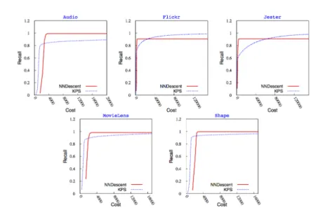
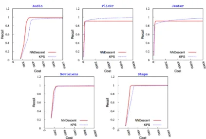
Fig. 2: Recall versus cost in KPS and NNDescent
We conducted the following experiments: (i) we evaluate the evolution of the recall against the cost; (ii) we measure the quality of the KNN graph by measuring the average similarity between a node and its k nearest neighbors against the cost; (iii) we compute the utility of the algorithm at each cycle; and (iv) as KPS and NNDescent operate in such a way that the size of the samples varies significantly, we artificially increase the size of the sample in KPS so that the same number of similarity computations is achieved for each node at each iteration in the two algorithms. Hence, we provide the recall figures for the two algorithms with similar cost.
4
Experimental Results
We now report on our experimental evaluation comparing KPS and NNDescent. Note that the experiments were run with k set to 20. We start with comparing the cost/recall tradeoff achieved by the two algorithms. We then study the quality of the KNN graph and the utility of each iteration. Finally, for the sake of fairness, we compare the convergence of the algorithms at equal cost.
4.1 Recall versus Cost
Figure 2 plots the recall as a function of the cost for both KPS and NNDescent. The cost here is measured as the total number of similarity computations. From figure 2, we observe that KPS exhibits a lower cost than NNDescent in sev-eral datasets i.e in Audio, MovieLens and Shape, while both approaches provide similar recall. We also observe that NNDescent does not always converge to the
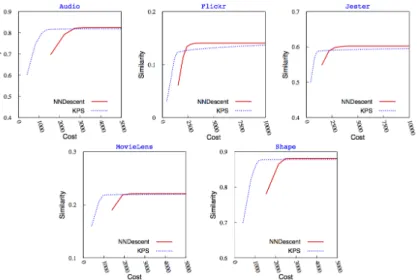
Fig. 3: Quality (Similarity) versus Cost in KPS and NNDescent
maximum recall. This is due to the fact that depending on the initial configura-tion and the operaconfigura-tion of NNDescent, the algorithm may reach a local minimum as shown on the Flickr and Jester datasets. On those two datasets, although slower, KPS converges. This is mainly due to the presence of random nodes in the candidate sets. In NNDescent instead, for some datasets, separated clusters are created during the algorithm operations. For Jester and Flickr, NNDescent does not exceed 90% of the recall.
In Audio, MovieLens and Shape, we observe that KPS reaches a similar recall than NNDescent at a much lower cost. For instance, for more than 0.8 recall, i.e. 80% of the KNN lists are similar to the ideal ones with a cost for KPS that is 42%, resp. 50%, resp. 51% lower in Audio, resp. MovieLens, resp. Shape. We also observe that in the datasets where NNDescent converges at a lower cost to a high recall, it never converges to the highest (Flickr and Jester). On the other hand, KPS might take too long to converge to an ideal KNN graph (Audio), as it might require comparisons with the whole system nodes.
These results suggest that KPS is an attractive alternative to NNDescent for reaching a high recall at low cost. Although this is out of the scope of this paper, it has been shown in many applications, e.g. collaborative filtering, that an ideal KNN graph is not necessarily required to achieve good performance in the recommendations. For instance, good recommendation quality can be achieved with a close to ideal KNN graph but not necessarily ideal.
4.2 Quality versus Cost
Regardless of the recall, another important metric is the quality of the KNN graph. For instance, consider a node provided with a non ideal KNN list, if the
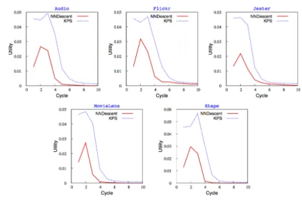
Fig. 4: Utility per cycle
similarity between that node and its neighbors is high, the KNN data might turn out to be as useful as the exact KNN.
We measure the quality of the KNN graph as the average similarity between a node and its neighbors in the KNN graph for both KPS and NNDescent. Figure 3 displays the quality against the cost for all datasets. We observe that KPS provides almost uniformly across all datasets a better quality at a much lower cost. Based on these results, we can also argue that the differences in recall observed in figure 2 are not significant. Effectively in Audio for instance, while NNDescent shows a better recall, the quality is similar in both KPS and NNDescent. This actually suggests that the discrepancy in recall is negligible: KPS provides k nearest neighbors of similar quality (although they are not the ideal neighbors). For instance, to achieve a Jester KNN graph with an average similarity equal to 0.59 (highest similarity), the cost needed in KPS is 2116 while it equals to 2748 for NNDescent. Moreover, KPS requires an average of 956 comparisons to achieve a MovieLens graph with 0.21 similarity, while NNDescent makes an average of 1919 comparisons to construct a graph with the same quality. Therefore, KPS exhibits a cost about ≈ 23%, resp. ≈ 49% lower for Jester, resp. MovieLens, than NNDescent.
The reason why NNDescent finds the ideal neighbors is due to the very large size of the candidate sets. KPS takes longer to converge because once the almost ideal neighbors are discovered, the graph hardly changes and the ideal neighbors are eventually reached through the presence of random nodes in the candidate set. Other factors related to the characteristics of the dataset, typically sparsity, can also impact the recall and the similarity achieved. We will come back to this issue in Section 4.5. This set of experiments shows that KPS achieves almost perfect KNN graph construction at a much lower cost than NNDescent.
4.3 Utility Study
To understand the impact of the candidate selection strategies used in KPS and NNDescent, we study the impact (utility) of each iteration on the KNN graph. Figure 4 plots the utility per cycle for all datasets. The utility tells us how useful similarity comparisons are at each cycle by measuring how many updates were generated (i.e. the number of discovered neighbors that achieves a better similarity). Utility is expressed as the ratio between the number of updates and the number of similarity comparisons. Results depicted in figure 4 are consistent over all datasets. Results clearly show that each iteration in KPS is much more useful than a NNDescent iteration. This is partly explained by the fact that NNDescent considers large candidate sets, especially for the first iterations, where its size is twice the size of the KPS candidate set. This also clearly shows that if the candidate set is carefully chosen, there is no need to consider large candidate sets.
After a few iterations, the evaluated utility of both protocols converges to 0. This is due to the usage of the boolean flag in NNDescent, and the selection rule in KPS (i.e. the usage of the number of updates to select neighbors of neighbors and random nodes). This also shows that the last steps to converge towards an ideal KNN graph take a very long time. This confirms the results depicted in figures 2 and 3: While KPS converges quickly to high quality neighborhoods, reaching the ideal neighborhoods takes much longer. This is a well-known problem in gossip-based sorting protocols [14].
4.4 Recall at Equal Cost
In the previous experiments, we compared KPS and NNDescent, in their orig-inal settings and as we mentioned before, KPS and NNDescent do not rely on candidate sets of similar sizes. NNDescent uses the nearest neighbors and the reverse nearest neighbors, whereas KPS is based only on the nearest neighbors and a few random nodes. In order to have a fair comparison between KPS and NNDescent, we now compare their recall under the same cost. Since, it is difficult to reduce the candidate set of NNDescent without altering the algorithm design, we increase the size of the candidate set of KPS by considering the 2k nearest neighbors for the candidate set.3
KPS, in its default setting, already presents best results in term of the quality, the cost and the utility metrics. Thus, we focus our comparison on the achieved recall. Figure 5 shows the recall of NNDescent and the modified version of KPS for all datasets. We then observe very similar results except for Jester and Flickr where KPS exceeds the NNDescent recall after few comparisons. This is due to the fact that NNDescent still suffers from the local minimum issue. This suggests that KPS naturally provides a reduced but relevant candidate set that is sufficient to achieve a high recall, an almost perfect quality at a low cost.
3 Note that the strength of KPS is to achieve good results with less information so
Fig. 5: Recall at equal cost (modified version of KPS with 40 nodes considered in the candidate set)
4.5 Discussion
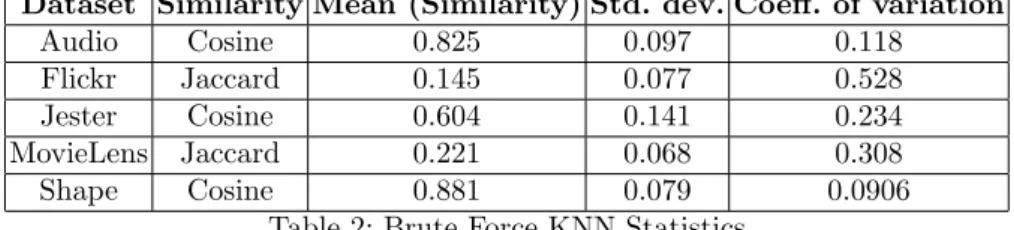
To understand, in more details, the behavior of KPS, we run the brute force KNN graph construction algorithm for each dataset and study the similarity on the obtained KNN graph. Table 2 shows the similarity characteristics of the ideal KNN graph of the considered datasets.
As shown in Table 2, the best KNN graphs of Shape and Audio have an average similarity respectively equals to 0.88 and 0.82, which represents a higher similarity compared to the average similarity of the other datasets. This means that the profiles in Audio and Shape tend to be very close to each other. Thus, exploring only neighbors of neighbors and the reverse neighbors of neighbors may lead to the comparison of a given node profile with all similar nodes in the system, which is quickly achieved by NNDescent since it relies on both the KNN and RNN lists. This explains the high recall achieved by NNDescent in these datasets. Whereas for datasets with a low average similarity, such as Flickr, the maximum recall achieved by NNDescent does not exceed 90%. In sparser datasets, more exploration of the graph is required to discover the closest nodes since similarity values between nodes have a lower value. KPS precisely provides better exploration capacities due to the use of random nodes. Therefore, KPS eventually ensures the highest possible recall for all datasets.
KPS provides a better quality/cost tradeoff than NNDescent since KPS achieves KNN graphs with higher similarities at a lower cost. Especially, in Audio and Shape (Figure 3), where the KPS’s KNN graph has the same quality as the one generated by NNDescent. For low average similarity datasets (e.g. Flickr), KPS converges rapidly to an approximate high quality KNN graph. Hence, one
Dataset Similarity Mean (Similarity) Std. dev. Coeff. of variation Audio Cosine 0.825 0.097 0.118 Flickr Jaccard 0.145 0.077 0.528 Jester Cosine 0.604 0.141 0.234 MovieLens Jaccard 0.221 0.068 0.308 Shape Cosine 0.881 0.079 0.0906
Table 2: Brute Force KNN Statistics
of the most important characteristic of KPS is to ensure convergence even for sparse datasets.
5
Related work
Centralized KNN approaches. Several works have been proposed to present effi-cient KNN graph construction algorithms. In [10], Chen & al. suggest divide and conquer methods for computing an approximate KNN graph. They make use of a Lanczos procedure to perform recursive spectral bisection during the divide phase. After each conquer step, an additional refinement step is performed to improve the accuracy of the graph. Moreover, a hash table is used to store the distance calculations during the divide and conquer process. Based on the same strategy (divide and conquer ), authors of [16] propose an algorithm that engages the locality sensitive hashing technique to divide items into small subsets with equal size, and then the KNN graph is computed on each subset using the brute force method. The divide and conquer principle was used in many other works such as [25]. On the other hand, several KNN graph construction approaches were based on a research index. In this direction, Zhong et al. [26] make use of a balanced search tree index to address the KNN search problem for a specific context in which the objects are locations in a road network. Paredes et al. [23] proposed a KNN graph construction algorithm for general metric space. The suggested algorithm is based on a recursive partition that builds a pre-index by performing a recursive partitioning of the space and on a pivot-based algorithm. Then, the index is used to solve a KNN query for each object. Most of these methods are either based on an additional index, or specific to a given similarity measure [11]. Moreover, they are designed for offline KNN graph construction, while KPS could be also used for online computation.
Gossip-based clustering. KPS is inspired from peer-to-peer gossip-based proto-cols. In such systems, each peer is connected to a subset of other peers in the network and periodically exchanges some information with one of its neighbors. While such protocols have been initially used to build uniform random topolo-gies [19, 21], they have also been applied in the context of several applications to cluster peers according to some specific metric (interest, overlap, etc) to build networks of arbitrary structure [18, 24] or to support various applications such
as query expansion [7], top-k queries [6] or news recommendation [9]. In such a system, the use of random nodes ensures that connectivity is maintained, each node is responsible to discover its KNN nodes by periodically exchanging neigh-borhood information with other peers. As opposed to KPS, such algorithms tend to limit the traffic on the network and therefore exchange information with one neighbor at a time, providing different convergence properties.
6
Conclusion
KNN graph computation is a core building block for many applications ranging from collaborative filtering to similarity search. Yet, in the Big Data era where the amount of information to process is growing exponentially, traditional algo-rithms hit the scalability wall. In this paper, we propose a novel KNN service, called KPS, which can be seen as a centralization of a peer-to-peer clustering ser-vice. KPS has been compared to NNDescent. The results show that KPS quickly reaches a close to optimal KNN graph while drastically reducing the complexity of the algorithm. Future works include applying KPS in dynamic settings where the attribute of nodes vary dynamically, inducing some changes in the similarity computation results. Clearly, providing a theoretical analysis of the convergence speed is a natural follow up research avenue.
References
1. Jester dataset. http://grouplens.org/datasets/jester/.
2. Jester joke recommender. http://shadow.ieor.berkeley.edu/humor/. 3. Movielens dataset. http://grouplens.org/datasets/movielens/.
4. D. Agrawal, S. Das, and A. El Abbadi. Big data and cloud computing: Current state and future opportunities. In Proceedings of the 14th International Conference on Extending Database Technology, EDBT/ICDT ’11, pages 530–533. ACM, 2011. 5. G. Amato and F. Falchi. Knn based image classification relying on local feature similarity. In Proceedings of the Third International Conference on SImilarity Search and APplications, SISAP ’10, pages 101–108. ACM, 2010.
6. X. Bai, R. Guerraoui, A.-M. Kermarrec, and V. Leroy. Collaborative personalized top-k processing. ACM Transactions on Database Systems, 36(4):26, 2011. 7. M. Bertier, D. Frey, R. Guerraoui, A.-M. Kermarrec, and V. Leroy. The
goss-ple anonymous social network. In Proceedings of the ACM/IFIP/USENIX 11th International Conference on Middleware, Middleware ’10, pages 191–211, 2010. 8. O. Boiman, E. Shechtman, and M. Irani. In defense of nearest-neighbor based
image classification. In Proceedings of the IEEE Conference on Computer Vision and Pattern Recognition, CVPR ’08, pages 1–8, 2008.
9. A. Boutet, D. Frey, R. Guerraoui, A. Jegou, and A.-M. Kermarrec. Whatsup: A decentralized instant news recommender. In Proceedings of the 27th IEEE Interna-tional Symposium on Parallel Distributed Processing, IPDPS ’13, pages 741–752, 2013.
10. J. Chen, H.-r. Fang, and Y. Saad. Fast approximate knn graph construction for high dimensional data via recursive lanczos bisection. The Journal of Machine Learning Research, 10:1989–2012, 2009.
11. M. Connor and P. Kumar. Fast construction of k-nearest neighbor graphs for point clouds. IEEE Transactions on Visualization and Computer Graphics, 16(4):599– 608, 2010.
12. C. Desrosiers and G. Karypis. A comprehensive survey of neighborhood-based recommendation methods. In Recommender Systems Handbook, pages 107–144. Springer, 2011.
13. W. Dong, C. Moses, and K. Li. Efficient k-nearest neighbor graph construction for generic similarity measures. In Proceedings of the 20th International Conference on World Wide Web, WWW ’11, pages 577–586. ACM, 2011.
14. G. Giakkoupis, A.-M. Kermarrec, and P. Woelfel. Gossip protocols for renaming and sorting. In Proceedings of the 27th International Symposium on Distributed Computing, pages 194–208. DISC’13, 2013.
15. G. Guo, H. Wang, D. Bell, Y. Bi, and K. Greer. Knn model-based approach in classification. In On The Move to Meaningful Internet Systems 2003: CoopIS, DOA, and ODBASE, volume 2888 of LNCS, pages 986–996. Springer, 2003. 16. K. Hajebi, Y. Abbasi-Yadkori, H. Shahbazi, and H. Zhang. Fast approximate
nearest-neighbor search with k-nearest neighbor graph. In Proceedings of the 22nd International Joint Conference on Artificial Intelligence, IJCAI ’11, pages 1312– 1317. AAAI Press, 2011.
17. M. J. Huiskes and M. S. Lew. The mir flickr retrieval evaluation. In Proceedings of the 1st ACM International Conference on Multimedia Information Retrieval, MIR ’08, pages 39–43. ACM, 2008.
18. M. Jelasity, A. Montresor, and O. Babaoglu. T-man: Gossip-based fast overlay topology construction. Computer Networks: The International Journal of Com-puter and Telecommunications Networking, 53(13):2321–2339, 2009.
19. M. Jelasity, S. Voulgaris, R. Guerraoui, A.-M. Kermarrec, and M. van Steen. Gossip-based peer sampling. The ACM Transactions on Computer Systems, 25(3), 2007.
20. V. Olman, F. Mao, H. Wu, and Y. Xu. Parallel clustering algorithm for large data sets with applications in bioinformatics. The IEEE/ACM Transactions on Computational Biology and Bioinformatics, 6(2):344–352, 2009.
21. R. Orm´andi, I. Heged˝us, and M. Jelasity. Overlay management for fully distributed user-based collaborative filtering. In Euro-Par 2010 - Parallel Processing, volume 6271 of LNCS, pages 446 – 457. Springer, 2010.
22. R. Pan, P. Dolog, and G. Xu. Knn-based clustering for improving social recom-mender systems. In Agents and Data Mining Interaction, volume 7607 of LNCS, pages 115–125. Springer, 2013.
23. R. Paredes, E. Ch´avez, K. Figueroa, and G. Navarro. Practical construction of k-nearest neighbor graphs in metric spaces. In Proceedings of the 5th International Conference on Experimental Algorithms, WEA ’06, pages 85–97. Springer, 2006. 24. S. Voulgaris and M. V. Steen. Vicinity: A pinch of randomness brings out the
structure. In Proceedings of the 14th ACM/IFIP/USENIX International Middle-ware Conference, MiddleMiddle-ware ’13, pages 21–40, 2013.
25. J. Wang, J. Wang, G. Zeng, Z. Tu, R. Gan, and S. Li. Scalable k-nn graph construc-tion for visual descriptors. In Proceedings of the IEEE Conference on Computer Vision and Pattern Recognition, CVPR ’12, pages 1106–1113, 2012.
26. R. Zhong, G. Li, K.-L. Tan, and L. Zhou. G-tree: An efficient index for knn search on road networks. In Proceedings of the 22Nd ACM International Conference on Information and Knowledge Management, CIKM ’13, pages 39–48. ACM, 2013.