HAL Id: hal-00690002
https://hal.archives-ouvertes.fr/hal-00690002v3
Submitted on 9 Jun 2012HAL is a multi-disciplinary open access
archive for the deposit and dissemination of sci-entific research documents, whether they are pub-lished or not. The documents may come from teaching and research institutions in France or
L’archive ouverte pluridisciplinaire HAL, est destinée au dépôt et à la diffusion de documents scientifiques de niveau recherche, publiés ou non, émanant des établissements d’enseignement et de recherche français ou étrangers, des laboratoires
Climbing on Pyramids
Jean Serra, Bangalore Ravi Kiran
To cite this version:
Climbing on Pyramids
Jean Serra and Bangalore Ravi Kiran Universit´e Paris-Est
Laboratoire d’Informatique Gaspard-Monge A3SI, ESIEE Paris, 2 Bd Blaise Pascal, B.P. 99
93162 Noisy-le-Grand CEDEX, France 15, march 2012
Abstract
A new approach is proposed for finding the ”best cut” in a hierarchy of partitions by energy minimization. Said energy must be ”climbing” i.e. it must be hierarchically and scale increasing. It encompasses separable energies and those composed under supremum.
1
Introduction
The present note1 extends the results of [15], which themselves generalize some results of L. Guigues’ Phd thesis [5] (see also [4]). In [5], any partition, or partial partition, of the space is associated with a ”separable energy”, i.e. with an energy whose value for the whole partition is the sum of the values over its various classes. Under this assumption, two problems are treated:
1. given a hierarchy of partitions and a separable energy ω, how to combine some classes of the hierarchy in order to obtain a new partition that minimizes ω?
2. when ω depends on integer j, i.e. ω = ωj, how to generate a sequence of minimum partitions that is increasing in j, which therefore should form a minimum hierarchy? Though L. Guigues exploited linearity and affinity assumptions to lean original models on, it is not sure that they are the very cause of the properties he found. Indeed, for solving problem 1 above, an alternative and simpler condition of increasingness is proposed in [15]. After additional developments, it leads to the theorem 4 of this paper. The second question, of a minimum hierarchy, which was not treated in [15], is the concern of sections 3 to 5 of the text. The main results are the theorem 12, and the new algorithm developed in Section 5, more general but simpler than that of [5]. It is followed by the two sections 6 and 7 about the additive and the ∨-composed energies respectively. They show that Theorem 12 applies to linear energies (e.g. Mumford and Shah, Salembier and Garrido), as well to several useful non linear energies (Soille, Zanoguera).
1
This work received funding from the Agence Nationale de la Recherche through contract ANR-2010-BLAN-0205-03 KIDIKO.
Figure 1: a) Basic input, b) and c) saliency maps from connected openings by dynamics [b)] and by volume [c)].
2
Hierarchy of partitions (reminder)
The space under study (Euclidean, digital, or else) is denoted by E, and the set of all partitions of E by D0(E). Here a convenient notion is that partial partition, of C. Ronse [10]. When we associate a partition π(A) of a set A ∈ P(E) and nothing outside A, then π(A) is called a partial partition of E of support A. The family of all partial partitions of set E is denoted by D(E), or simply by D when there is no ambiguity.
Finite hierarchies of partitions appeared initially in taxonomy, for classifying objects. One can quote in particular the works of J.P. Benz´ecri [2] and of E. Diday [3]. We owe to the first author the theorem linking ultrametrics with hierarchies, namely the equivalence between statements 1 and 3 in theorem 2 below. Hierarchies H of partitions usually derive from a chain of segmentations of some given function f on set E, i.e. from a stack of scalar or vector images, a chain which then serves as the framework for further operators. We consider, here, function f and hierarchy H as two starting points, possibly independent. This results in the following definition:
Definition 1 Let D0(E) be the set of all partitions of E, equipped with the refinement
or-dering. A hierarchy H, of partitions πi of E is a finite chain in D0(E), i.e.
H = {πi, 0 ≤ i ≤ n, πi ∈ D0(E) | i ≤ k ≤ n ⇒ πi ≤ πk}, (1)
of extremities the universal extrema of D0(E), namely π0 = {{x}, x ∈ E} and πn= E. Let Si(x) be the class of partition πi of H at point x ∈ E. Denote by S the set of all classes Si(x) , i.e. S = {Si(x), x ∈ E, 0 ≤ i ≤ n}. Expression (1) means that at each point x ∈ E the family of those classes Si(x) of S that contain x forms a finite chain Sx in P(E),
Figure 2: The initial image has been transformed by increasing alternated connected filters. They result in partitions into flat zones that increase from left to right.
Figure 3: Left, hierarchical tree; right, the corresponding space structure. S1 and S2 are the nodes sons of E, and H(S1) and H(S1) are the associated sub-hierarchies. π1 and π2are cuts of H(S1) and H(S1) respectively, and π1⊔ π2 is a cut of E.
of nested elements from {x} to E :
Sx = {Si(x), 0 ≤ i ≤ n}.
According to a classical result, a family {Si(x), x ∈ E, 0 ≤ i ≤ n} of indexed sets generates the classes of a hierarchy iff
i ≤ j and x, y ∈ E ⇒ Si(x) ⊆ Sj(y) or Si(x) ⊇ Sj(y) or Si(x) ∩ Sj(y) = ∅. (2) A hierarchy may be represented in space E by the saliencies of its frontiers, as depicted in Figure 1. Another representation, more adapted to the present study, emphasizes the classes rather than their edges, as depicted in Figure2. Finally, one can also describe it, in a more abstract manner, by a family tree where each node of bifurcation is a class S, as depicted in Figure 3. The classes of πi−1 at level i − 1 which are included in Si(x) are said to be the
sons of Si(x). Clearly, the sets of the descenders of each S forms in turn a hierarchy H(S) of summit S, which is included in the complete hierarchy H = H(E).
The two zones H(S1) and H(S2), drawn in Figure 3 in small dotted lines, are examples of such sub hierarchies. The following theorem [15] makes more precise the hierarchical structure
Theorem 2 The three following statements are equivalent: 1. H is an indexed hierarchy,
2. the set S of all classes of the partition πi of H forms an ultrametric space, of distance
the indexing parameter,
3. every binary criterion σ : (F, S ∪ ∅) → {0, 1} is connective.
This result shows that the connective segmentation approach is inefficient for hierarchies, and orients us towards the alternative method, which consists in optimizing an energy.
3
Optimum partitioning of a hierarchy
3.1 Cuts in a hierarchy
Following L. Guigues [5] [4], we say that any partition π of E whose classes are taken in S defines a cut in hierarchy H. The set of all cuts of E is denoted by Π(E) = Π. Every ”horizontal” section πi(H) at level i is obviously a cut, but several levels can cooperate in a same cut, such as π(S1) and π(S2), drawn with thick dotted lines in Figure 3. Similarly, the partition π(S1) ⊔ π(S2) generates a cut of H(E). The symbol ⊔ is used here for expressing that groups of classes are concatenated. It means that given two partial partitions π(S1) and π(S2) having disjoint supports, π(S1) ⊔ π(S2) is the partial partition whose classes are either those of π(S1) or those of π(S2).
Similarly, one can define cuts inside any sub-hierarchy H(S) of summit S. Let Π(S) be the family of all cuts of H(S). The union of all these families, when node S spans hierarchy H is denoted by
e
Π(H) = ∪{Π(S), S ∈ S(H)}. (3)
Although the set eΠ(H) does not regroup all possible partial partitions with classes in S, it contains the family Π(E) of all cuts of H(E). The hierarchical structure of the data induces a relation between the family Π(S) of the cuts of node S and the families Π(T1), .., Π(Tq) of the sons T1, .., Tq of S. Since all expressions of the form ⊔{π(Tk); 1 ≤ k ≤ q} define cuts of S, Π(S) contains the whole family
Π′
(S) = {π(T1) ⊔ ..π(Tk).. ⊔ π(Tq); π(T1) ∈ Π(T1)... π(Tq) ∈ Π(Tq)},
plus the cut of S into a unique class, i.e. S itself, which is not a member of Π′(S). And as the other unions of several Tk are not classes listed in S, there is no other possible cut, hence
Π(S) = Π′(S) ∪ S. (4)
3.2 Cuts of minimum energy and h-increasingness
In the present context, an energy ω : D(E) → R+is a non negative numerical function over the family D(E) of all partial partitions of set E. The cuts of Π(E) ⊆ eΠ of minimum energy, or minimum cuts, are characterized under the assumption of hierarchical increasingness, or more shortly of h-increasingness [15].
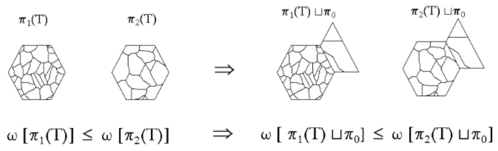
Figure 4: Hierachical increasingness.
Definition 3 Let π1 and π2 be two partial partitions of same support, and π0 be a partial
partition disjoint from π1 and π2. An energy ω on D(E) is said to be hierarchically increasing, or h-increasing, in D(E) when, π0, π1, π2 ∈ D(E), π0 disjoint of π1 and π2, we have
ω(π1) ≤ ω(π2) ⇒ ω(π1⊔ π0) ≤ ω(π2⊔ π0). (5) An illustration of the meaning of implication (5) is given in Figure 4. When the partial partitions are embedded in a hierarchy H, then Rel.(5) allows us an easy characterization of the cuts of minimum energy of H, according to the following property, valid for the class H of all finite hierarchies on E
Theorem 4 Let H ∈ H be a finite hierarchy, and ω be an energy on D(E). Consider a node S of H with p sons T1..Tp of minimum cuts π∗
1, ..πp∗. The cut of minimum energy of node S
is either the cut
π∗1⊔ π ∗ 2.. ⊔ π
∗
p, (6)
or the partition of S into a unique class, if and only if S is h-increasing.
Proof. We firstly prove that the condition is sufficient. The h-increasingness implies of the energy implies that cut (6) has the lowest energy among all the cuts of type Π′(S) = ⊔{π(Tk); 1 ≤ k ≤ p} (it does not follow that it is unique). Now, from the decomposition (4), every cut of S is either an element of Π′(S), or S itself. Therefore, the set formed by the cut (6) and S contains one minimum cut of S at least.
We will prove that the h-increasingness is necessary by means of a counter-example. Consider the hierarchies of n levels in E = R2
, and associate an energy with the lengths of the frontiers as follows
ω(π(S)) = ω(T1⊔ ..Tu.. ⊔ Tq) = X 1≤u≤q (∂Tu), when X 1≤u≤q (∂Tu) ≤ 5 (7) ω(π(S)) = X 1≤u≤q (∂Tu) − 5 when not.
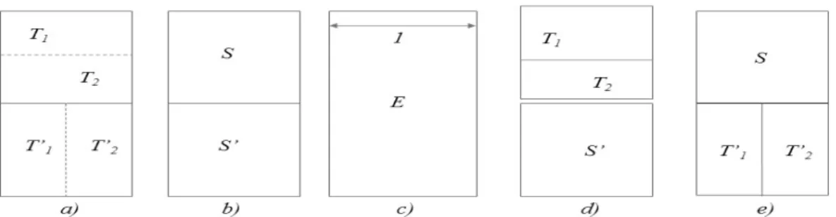
where {Tu, 1 ≤ u ≤ q} are the sons of node S. Calculate the minimum cut of the three levels partition depicted in Fig.5 a) b) and c). The size of the square is 1 and one must take half the
Figure 5: a), b),c): three levels of a hierarchy H. Partition a) is the minimum cut for energy (7), which contradicts hierarchical increasingness. Partitions d) and e) are two minimum cuts of H for the sequence (15) of energies. They contradict scale increasingness.
length for the external edges. We find ω(T1⊔ T2) = 3 and ω(S) = 2. Hence S is the minimum cut of its own sub-hierarchy. So does S′. At the next level we have ω(S ⊔ S′) = 4, and ω(E) = 3. Nevertheless, E is not the minimum cut, because ω(T1⊔ T2⊔ T1′⊔ T2) = 6 − 5 = 1!′
The condition of h-increasingness (5) opens into a broad range of energies, and is easy to check. It encompasses the case of the separable energies [5] [13], as well as energies composed by suprema [1] [16] [18]. Computationally, it yields to the following Guigues’algorithm:
• scan in one pass all nodes of H according to an ascending lexicographic order ; • determine at each node S a temporary minimum cut of H by comparing the energy of
S to that of the concatenation of the temporary minimum cuts of the (already scanned) sons Tk of S .
3.3 Single minimum cuts
It may happen that in the family Π(S) of Relation (4) a minimum cut of Π′(S) has the same energy as that of S. This event introduces two solutions which are then carried over the whole induction. And since such a doublet can occur regarding any node S of H, the family M = M (H) of all minimum cuts may be very comprehensive. However, M turns out to be structured as a complete lattice for the ordering of the refinement, where the sup (resp. the inf) are obtained by taking the union (resp. the intersection) of the classes.
The risk of several minimum cuts w.r.t. ω may becomes sometimes cumbersome. Then one can always ensure unicity by slightly modifying a h-increasing energy ω. Denote by m the minimum of all the positive differences of energies involved in the partial partitions of H, i.e.
m = inf{ω(π) − ω(π′), ω(π) < ω(π′
)} π, π′
∈ eΠ(H).
As the cardinal of eΠ is finite, m is strictly positive. Therefore, one can find a ε such as 0 < ε < m, and state the following:
Proposition 5 Let ω be a h-increasing energy over eΠ. Introduce the additional energy ω′
for all {π(S) ∈ Π(S), S ∈ S}
ω′[π(S)] = ε, π(S) 6= {S} ω′[S] = 0,
with 0 < ε < m. Then the sum ω + ω′ is h-increasing and associates a unique minimum cut
with each sub-hierarchy H(S). When ω[π∗(S)] 6= ω[{S}], then the minimum cut for ω + ω′
is π∗
(S), and it is {S} itself when {S} and π∗(S) have the same ω-energy.
ω[π∗(S)] 6= ω[{S}] ⇒ π∗(S) best cut (8) ω[π∗
(S)] = ω[{S}] ⇒ {S} best cut
Proof. Let us denote by small letters the main inequalities of the proof (a) ω(π1) ≤ ω(π2)
(b) ω(π1⊔ π0) ≤ ω(π2⊔ π0) (c) ω(π1) + ω′(π1
) ≤ ω(π2) + ω′(π2)
(d) ω(π1⊔ π0) + ω′(π1⊔ π0) ≤ ω(π2⊔ π0) + ω′(π2⊔ π0)
We suppose that (a) ⇒ (b), and must prove that then (c) ⇒ (d). Let S0 be the support of partition π0. Note firstly that the equalities ω′(π1
⊔ π0) = ω′(π2
⊔ π0) = ε always hold, since π1⊔ π0 6= {S ∪ S0} and π2⊔ π0 6= {S ∪ S0}. Distinguish three cases:
1/ π16= {S} and π26= {S}. Obviously, (c) ⇒ (a) ⇒ (b) ⇒ (d); 2/ π16= {S} and π2= {S}. Again, (c) ⇒ (a) ⇒ (b) ⇒ (d);
3/ π1 = {S} and π2 6= {S}. Inequality (c) becomes ω(π1) ≤ ω(π2)+ ε. If ω(π1) > ω(π2), then ω(π1) ≥ ω(π2) + m > ω(π2) + ε, which is impossible, hence ω(π1) ≤ ω(π2). This implies, as previously, (b) and then (c).
Note that the impact of ω′ is reduced to the case of equality ω[π∗
(S)] = ω[{S}], and that ω+ ω′ can be taken arbitrary close to ω, but different from it. Proposition 5 turns out to be a particular case of the more general, and more useful result
Corollary 6 Define the additive energy ω′ by the relations
ω′[π(S)] = ε, when π(S) 6= {S} and ω[π(S)] ≤ ω0 ω′[π(S)] = 0, when π(S) = {S} and ω[π(S)] ≤ ω0 ω′[π(S)] = ε, when π(S) = {S} and ω[π(S)] > ω0 ω′[π(S)] = 0, when π(S) 6= {S} and ω[π(S)] > ω0. Then ω + ω′
Proof. When ω[π(S)] ≤ ω0, we meet again the previous proposition 5. When ω[π(S)] > ω0, then we still have the triple distinction of the previous proof, the only difference being that case 2/ and 3/ are inverted, which achieves the proof.
Unlike in Proposition 5, in case of equality ω[π∗(S)] = ω[{S}], the optimum cut is now {S} when ω[π(S)] ≤ ω0 and π∗(S) when not. Corollary 6 is used for example for proving that Soille’s energy is h-increasing in section 7.1 below.
The result (8) is a top-down property:
Proposition 7 Let π∗(E) be the single minimum cut of a hierarchy H w.r. to a h-increasing
energy ω, and let S be a node of H. If π∗(E) meets the sub-hierarchy H(S) of summit S,
then the restriction π∗(S) of π∗(E) to H(S) is the single minimum cut of the sub-hierarchy H(S).
Proof. We have to prove Relation (8). If π∗(S) = S, then the relation is obviously satisfied. Suppose now that the restriction π∗(S) is different from S, and that there exists a cut π0 of S with ω(π0) ≤ ω(π∗(S)). Denote by π− the partial partition obtained when π∗(S) is removed from π∗(E). The h-increasingness then implies that ω(π0
⊔ π−
) ≤ ω(S ⊔ π−) = ω(π∗(E)). But by definition of π∗(E) we also have the reverse inequality, hence ω(π0⊔ π−) = ω(π∗(E)). Now, this equality contradicts the Relation (8) applied to the whole space E, so that the inequality ω(π0) ≤ ω(π∗(S)) is impossible, and ω(π0) > ω(π∗(S)) for all π0∈ Π(S).
3.4 Generation of h-increasing energies
As we saw, the energy ω : D(E) → R+
is defined on the family D(E) of all partial partitions of E. An easy way to obtain a h-increasing energy consists in defining it, firstly, over all sets S ∈ P(E), considered as one class partial partitions {S}, and then in extending it to partial partitions by some law of composition. Then, the h-increasingness is introduced by the law of composition, and not by ω[P(E)]. The first two modes of composition which come to mind are, of course, addition and supremum, and indeed we can state
Proposition 8 Let E be a set and ω : P(E) → R+
an arbitrary energy defined on P(E), and let π ∈ D(E) be a partial partition of classes {Si, 1 ≤ i ≤ n}. Then the the two extensions of ω to the partial partitions D(E)
ω(π) = ∨{ω(Si), 1 ≤ i ≤ n} and ω(π) =P{ω(Si), 1 ≤ i ≤ n}
are h-increasing energies.
We shall study these two models in sections 6 and 7, when they depend on a parameter leading to multiscale structures. A number of other laws are compatible with h-increasingness. Instead of the supremum and the sum one could use the infimum, the product, the difference sup-inf, the quadratic sum, and their combinations. Moreover, one can make depend ω on more than one class, on the proximity of the edges, on another hierarchy, etc..
3.5 Stucture of the h-increasing energies
We now analyze how different h-increasing energies interact on a same hierarchy. The family Ω of all mappings ω : D →R+
forms a complete lattice where ω ≤ ω′ ⇔ ω(π) ≤ ω′(π) for all π ∈ D
and whose extrema are ω(π) = 0 and ω(π) = +∞. What can be said about the sub class of Ω′
⊆ Ω of the h-increasing energies? The class Ω′ is obviously closed under addition and multiplication by positive scalars, i.e.
{ωj} ⊆ Ω′, λj ≥ 0 ⇒ Pλjωj ∈ Ω′ (9) Consider now a finite family {ωi, i ∈ I} in Ω′such that, for π0, π1, π2 ∈ D(E), π
0disjoint of π1 and π2, we have
ωi(π1) ≤ ωj(π2) ⇒ ωi(π1⊔ π0) ≤ ωj(π2⊔ π0), π0, π1, π2 ∈ D (10) a relation that generalizes the h-increasingness (5).
Proposition 9 The family of those energies that satisfy implication (10) is a finite sub-lattice
Ω′
of Ω, and for any family {ωi, i ∈ I} in Ω′ we have
(∧ωi)(π) ≤ (∧ωi)(π′) ⇒ (∧ωi)(π ⊔ π0) ≤ (∧ωi)(π′⊔ π0) (11) (∨ωi)(π) ≤ (∨ωi)(π′)
⇒ (∨ωi)(π ⊔ π0) ≤ (∨ωi)(π′⊔ π0) (12)
Proof. Consider a family {ωi, i ∈ I} which satisfy the h-increasingness (10). Suppose that (∧ωi)(π) ≤ (∧ωi)(π′), and let i0 be the parameter of the smallest of the ωi(π). Then we have ωi0(π) ≤ ωi(π
′), i ∈ I, hence, from Rel.(10), ω
i0(π ⊔ π0) ≤ ωi(π
′ ⊔ π0), so that ωi0(π ⊔ π0) ≤ (∧ωi)(π
′
⊔ π0), and finally (∧ωi)(π ⊔ π0) ≤ (∧ωi)(π′⊔ π0). Energy (∧ωi) is thus h-increasing. Same proof for the supremum.
Note that the infimum cut π∧ωi related to energy ∧ωi is not the infimum ∧π
∗
ωi of the
minimum cuts generated by the ωi. It has to be computed directly (dual statement for the supremum).
4
climbing energies
The usual energies are often given by finite sequences {ωj, 1 ≤ j ≤ p} that depend on a positive index, or parameter, j. Therefore, the processing of hierarchy H results in a sequence of p optimum cuts πj∗, of labels 1 ≤ j ≤ p. A priori, the πj∗ are not ordered, but is they were, i.e. if
j ≤ k ⇒ πj∗≤ πk∗, j, k ∈ J,
then we should obtain a nice progressive simplification of the optima. We now seek the conditions that permit such an increasingness.
Consider a finite family of energies {ωj, 1 ≤ j ≤ p} on all partial partitions D(E) of set E , and apply these energies to the partial partitions eΠ(H) of hierarchy H (Relation (3)). The family {ωj}, not totally arbitrary, is supposed to satisfy the following condition of scale
increasingness:2
Definition 10 A family of energies {ωj, 1 ≤ j ≤ p} on D(E) is said to be scale increasing
when for j ≤ k, each support S ∈ S and each partition π ∈ Π(S), we have that
j ≤ k and ωj(S) ≤ ωj(π) ⇒ ωk(S) ≤ ωk(π), S ∈ P(E). (13) In case of a hierarchy H, relation (13) means that, if S is a minimum cut w.r. to energy ωj for a partial hierarchy Π(S), then S remains a minimum cut of Π(S) for all energies ωk, k ≥ j. As j increases, the ωj’s preserve the sense of energetic differences between the nodes of hierarchy H and their partial partitions. In particular, all energies of the type ωj = jω are scale increasing.
Axiom (13) compares two energies at the same level of H, whereas axiom (5) allows us to compare a same energy at two different levels. Therefore, the most powerful energies should to be those which combine scale and h-increasingness, i.e.
Definition 11 We call climbing energy any family {ωj, 1 ≤ j ≤ p} of energies over eΠ which
satisfies the three following axioms, valid for ωj, 1 ≤ j ≤ p and for all π ∈ Π(S), S ∈ S • i) h-increasingness, i.e. relation(5):
ωj(π1) ≤ ωj(π2) ⇒ ωj[(π1⊔ π0] ≤ ωj[(π2⊔ π0], π1, π2∈ H(S)
• ii) single minimum cutting, i.e. relation(??):
either ωj[π∗(S)] < ωj(π), or π∗(S) = S,
• iii) scale increasingness, i.e. relation(13) :
j ≤ k and ωj(S) ≤ ωj(π) ⇒ ωk(S) ≤ ωk(π), π ∈ H(S).
Under these three assumptions, the climbing energies satisfy the very nice property to order the minimum cuts with respect to the parameter j, namely:
Theorem 12 Let {ωj, 1 ≤ j ≤ p} be a family of energies, and let πj∗ (resp. πk∗) be the
minimum cut of hierarchy H according to the energy ωj (resp. ωk). The family {πj∗,1 ≤ j ≤ p} of the minimum cuts generates a unique hierarchy H∗ of partitions, i.e.
j ≤ k ⇒ πj∗ ≤ πk∗, 1 ≤ j ≤ k ≤ p (14)
if and only if the family {ωj} is a climbing energy.
2
Scale increasingness is called by L.Guigues ”partial causality” in [5], p.161, where it appears as a conse-quence and not as a starting point.
Proof. Assume that axiom iii) of a climbing energy is satisfied, and denote by Sj and Sk the two classes of πj∗ and πk∗ at a given point x. According to Rel.(2), we must have either Sj ⊆ Sk or Sk ⊂ Sj. We will prove that the second inclusion is impossible. Suppose that class Sk ⊂ Sj. Then the restriction of the minimum cut πk∗ to Sj generates a cut, π0 say, of Sj. According to proposition 7, which involves axioms i) and ii) of a climbing energy, the restriction π0 is in turn minimum for the energy ωk over Π(Sj), i.e. ωk(π0) < ωk(Sj). This implies, by scale increasingness, that ωj(π0) < ωj(S
j) (here Relation (13) has been red from right to left). But this inequality contradicts the fact that Sj is a minimum cut for its own hierarchy H(Sj). Therefore the inclusion Sk ⊂ Sj is rejected, and the alternative inclusion Sj ⊆ Sk is satisfied whatever x ∈ E, which results in πj∗ ≤ πk∗. Moreover, because of the single minimum cutting axiom, each πj∗ being unique, so does the whole hierarchy H∗.
The ”only if” statement will be proved by means of a counter-example. The notation is the same as in system (7) but we add a term for the areas and we replace the length ∂Tu of the frontier of each Tu by the length ∂horTu (resp. ∂vertTu) of the horizontal (resp. vertical) projection of the said frontiers if j ≤ j0, (resp. if j > j0).
ωj(π(S)) = ω(T1⊔ ..Tu.. ⊔ Tq) = 4 X 1≤u≤q (areaTu)2+ 2 X 1≤u≤q (∂horTu), when j ≤ j0 (15) ωj(π(S)) = ω(T1⊔ ..Tu.. ⊔ Tq) = 4 X 1≤u≤q (areaTu)2 + 2 X 1≤u≤q (∂vertTu), when j > j0,
(border lengths being divided by 2). For each value of j, the energy ωj1 is h-increasing, and one can apply proposition 5 for ensuring unicity. However, if j ≤ j0 then ω(T1 ⊔ T2) = 6, ω(T′
1⊔ T2′) = 4, ω(S) = ω(S′) = 6, ω(E) = 19. Therefore the minimum cut is the partition T′
1⊔ T2′⊔ S, depicted in Figure 5 d). By symmetry, if j > j0 then the minimum cut becomes T1 ⊔ T2 ⊔ S′, of Figure 5 c). Now these two cuts are not comparable, which contradicts implication (14).
Relation (14) has been established by L. Guigues in his Phd thesis [5] for affine and separable energies, called by him climbing energies. However, the core of the assumption (13) concerns the propagation of energy through the scales (1...p), rather than affinity or linearity, and allows non additive laws (see Section 7). In addition, the new climbing axioms 11 lead to the algorithms of the next section, much simpler than that of [5].
The scale sequence has been supposed finite, i.e. with 1 ≤ j ≤ p. We could replace j by a positive parameter λ ∈ R+. But the induction method for finding the optimal cut requires a finite hierarchy H. Therefore the number of the scale parameters actually involved in the processing of H will always be finite.
5
Implementation via a pedagogical example
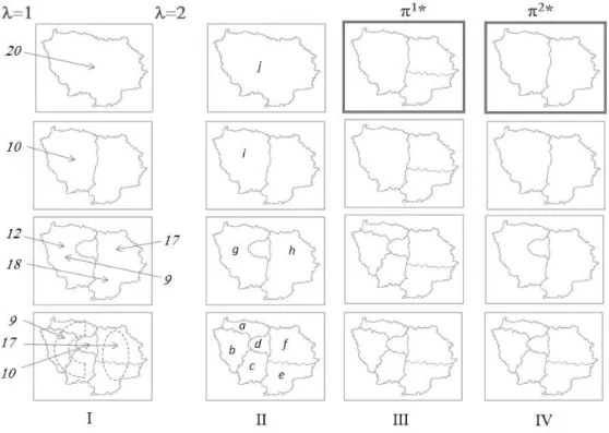
We now describe step by step two algorithms for generating a hierarchy of minimum cuts. The input hierarchy H comprises the four levels and two energies {ω1, ω2} depicted in Figure 6. The energies of the classes are given along column I, left for λ = 1, and right for the energies
Figure 6: Column I: initial hierarchy and associated energies (left, for λ = 1; right, the changes for λ = 2); column II: reading order; columns III and IV: progressive extraction of the minimum cuts for λ = 1 and λ = 2, the two final minuma have bold frames.
that are different for λ = 2.They are composed by supremum (the energies of the three partial partitions {a, b, c}, and {e, f } are not decomposed). If class S is temporary minimum for ωλ then is remains temporary minimum for all ωµ, µ ≥ λ. The scale of apparition λ+(S) = inf{λ | S temporary minimum for ωλ} is the smallest λ for which S is a temporary minimum. A class S which is covered by a temporary minimum class Y at scale µ remains covered by temporary minima at all scales ν ≥ µ. The scale of removal λ−(S) = min{λ+
(Y ), Y ∈ H, S ⊆ Y } is the smallest µ for which S is covered. Therefore, if λ+(S) < λ−(S), then class S ∈ H belongs to the minimum cuts πλ∗for all λ of the interval of persistence [λ+
(S), λ−(S)]. If λ−
(S) ≤ λ+
(S), then S, non-persistent, never appears as a class of a minimum cut. This happens to class g, for which λ−(g) = 1 and λ+(g) = 2.
When the two bounds λ+
(S) and λ−
(S) are known for all classes S ∈ H then the hierarchy of the minimum cuts πλ∗is completely determined.They are calculated in two passes as follows 1-take the nodes following their labels (ascending pass). For node S, calculate the two energies ωλ of S and of its sons π(S), for λ = 1, 2. Stop at the first λ such that ωλ(S) ≤ ωλ(π(S)). This value is nothing but λ+(S). Continue for all nodes until he top of the hierarchy. This pass provides the λ+
(S) values for all S ∈ H. In Figure 6 the sequence of the two energies is climbing: when a class is temporary minimum for λ = 1, it also does for λ = 2. Two changes occur from λ = 1 to λ = 2 : g and h have now the same energies as {a, b, c} and {e, f }respectively.
2-The second pass progresses top down. Each class Y is compared to its sons Z1, .Zi, and one allocates to each son Zi the new value min{λ−(Y ), λ−(Zi
)}. At the end of the scan, all values λ−(S) are known.
6
Additive energies
The additive mode was introduced and studied by L.Guigues under the name of separable
energies [5]. All classes S of S are supposed to be connected. Denote by {Tu, 1 ≤ u ≤ q} the q sons which partition the node S, i.e. π(S) = T1⊔ ..Tu.. ⊔ Tq. Provide the simply connected sets of P(E) with energy ω, and extend it from P(E) to the set D(E) of all partial partitions by using the sums
ω(S) = ω(T1⊔ ..Tu.. ⊔ Tq) = q X
1
ω(Tu). (16)
All separable energies ω are clearly h-increasing on any hierarchy, since one can decompose the second member of implication (5) into ω(π1⊔ π0) = ω(π1) + ω(π0), and ω(π2⊔ π0) = ω(π2) + ω(π0). However, they do not always lend themselves to multiscale structures, and a supplementary assumption of affinity has to be added [5], by putting
ωj(S) = ωµ(S) + λjω∂(S) S ∈ S (17)
where ωµ is a goodness-of-fit term, and ω∂ a regularization one, and λj ≥ 0 an increasing function of j. The term ωµ is associated with the interior of A and ω∂ with its boundary. In such an affine energy, the function ω∂ must be c-additive on the boundary arcs F , in the sense of integral geometry, i.e. one must have
since most of the arcs F1, F2, ...Fi of the boundaries are shared between two adjacent classes. The passage ”set→partial partition” can then be obtain by the summation (16). One clas-sically take for ω∂ the arc length function (e.g. in Rel.(20) ), but it is not the only choice. Below, one of the examples by Salemenbier and Garrido about thumbnails uses ω∂(S) = 1. One can also think about another ω∂(S), which reflects the convexity of A.
The axiom (13) of scale increasingness involves only increments of the energy ω, which suggests the following obvious consequence:
Proposition 13 If a family {ωj, 1 ≤ j ≤ p} of energies is scale increasing, then any family {ωj + ω0, 1 ≤ j ≤ p}, where ω
0 is an arbitrary energy over eΠ which does not depends on j,
is in turn scale increasing.
6.1 Additive energy and convexity
Consider, indeed, in R2 a compact connected set X without holes, and let dα be the elemen-tary rotation of its outward normal along the element du of the frontier ∂X. As the radius of curvature R equals du/dα, and as the total rotation of the normal around ∂X equals π, we have 2π = Z R≥0 du R(u)+ Z R>0 du |R(u)|. (19)
When dealing with partitions, the distinction between outward and inward vanishes, but the parameter n(X) = 1 2π Z ∂X du |R(u)|
still makes sense. It reaches its minimum 1 when set X is convex, and increases with the degree of concavity. For a starfish with 5 pesudo-podes, it values around 5. Now n(X) is c-additive for the open parts of contours, therefore it can participate as a supplementary term in an additive energy. In digital implementation, the angles between contour arcs must be treated separately (since c-additivity applies on the open parts).
6.2 Mumford and Shah energy
Let π(S) be the partition of a summit S into its q sons {Tu, 1 ≤ u ≤ q} i.e. π(S) = T1⊔ ..Tu.. ⊔ Tq. The classical Mumford and Shah energy ωj on π(S) and w.r.t. a function f comprises two terms [7]. The first one sums up the quadratic differences between f and its average m(Tu) in the various Tu, and a second term weights by λj the lengths ∂Ti of the frontiers of all Tu, i.e.
ωj(π(S)) = X 1≤u≤q Z x∈Tu k f (x) − m(T u) k2 +λj X 1≤u≤q (∂Tu) = ωµ(π) + λjω∂(π) (20)
where the weight λj is a numerical increasing function of the level number j. Both increas-ingness relations (5) and (13) are satisfied and Theorem 12 applies to the additive energy (20).
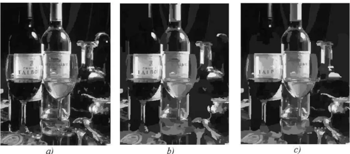
Figure 7: Minimum cuts of the hierarchy Fig. 1d, for two compression rates of 25 and 55 applied to the luminance ( a) and b) respectively); c) for a compression rate of 55 applied to the chrominance.
6.2.1 Additive energies and Lagrangian
The example of additive energy that we now develop is an extension of the creation of thumbnails by Ph. Salembier and L. Garrido [13] [14], itself based on Equation (20). We aim to generate ”the best” simplified version of the image f of Fig. 1, in its color version of components (r; g; b), for the compression rate ρ ≃ 25. The bit depth of f is 24 and its size is 320 × 416 pixels. The hierarchy H of f is that depicted, via its saliency map, in Fig. 1d. It has been obtained from the luminance l = (r + g + b)/3. In each class S of H, the reduction consists in replacing the function f by its mean m(l) in S. The quality of this approximation is estimated by the L2 norm, i.e.
ωµ(S) =X x∈S
k l(x) − m(S) k2 (21)
If the coding cost for a frontier element is c, that of the whole class S becomes ω∂(S) = 24 +
c
2 | ∂S | (22)
with 24 bits for m(S), and we take c = 2 for elementary cost. The total energy of a cut π is thus written ωj(π) = ωµ(π) + λjω
∂(π). By applying Lagrange’s theorem, we observe that the problem of finding the minimum of ωµ(π) under the constraint ω∂(π) ≃ 25 implies that the Lagrangian ωµ(π) + λjω∂(π) is a minimum. In this equation, the level j is unknown, but as the ωj are multiscale, we can easily calculate the sequence {πj∗, 1 ≤ j ≤ p} of the minimum cuts. Moreover, the term ω∂(π) itself turns out to be a decreasing function of j and λj, so that the solution of the Lagrangian is the πj∗ whose term ω∂(πj∗) is the greatest one smaller than k. It is depicted in Fig.7 a (in a black and white version).
Classically one reaches the Lagrangian minimum value by means of a system of partial derivatives. Now, remarkably, the present approach replaces the of computation of derivatives by a climbing. Moreover, we have under hand, at once, all best cuts for all compression rates. If we take ρ ≃ 55 for example, we find the image of Fig.7 b, whose partition is located at a higher level in the same pyramid of the best cuts. L. Guigues was the first to point out this nice property [5].
There is no particular reason to choose the same luminance l for generating the pyramid and, later, as the quantity to involve in the quality (21) to minimize. In the RGB space, a colour vector −→x (r; g; b) can be decomposed in two orthogonal projections
i ) on the grey axis, namely−→l of components (l/3; l/3; l/3),
ii ) and on the chromatic plane orthogonal to the grey axis at the origin, namely −→c of components(3/√2)(2r − g − b; 2g − −b − r; 2b − r − g).
We have −→x =−→l + −→c . The optimization is obtained by replacing the luminance l(x) in (21) by the module | −→c (x) | of the chrominance at point x. We now find for best cut the segmentation depicted in Fig.7 c, where, for the same compression rate ρ ≃ 55, color details are better rendered (e.g. right bottom), but black and white parts are worse (e.g. the letters on the labels).
7
Energies composed by supremum
We now us go back to Rel.(16), and replace the sum by a supremum. It gives:
ω(S) = (T1⊔ ..Tu.. ⊔ Tq) = q _
1
ω(Tu).
This time the second member of implication (5) is written ω[(π1⊔ π0] = ω(π1) ∨ ω(π0), and ω[(π2⊔ π0] = ω(π2) ∨ ω(π0), so that ω is h-increasing. The property remain true when ∨ is replaced by ∧.
7.1 Connective segmentation under constraint
This method was proposed by P. Soille and J. Grazzini in [16] and [17] with several variants; it is re-formulated by C. Ronse in a more general framework in [12]. Start from a hierarchy H and a numerical function f . Define the energy ωj for class S by
ωj(S) = 0 when sup{f (x), x ∈ S} − inf{f (x), x ∈ S} ≤ cj ωj(S) = 1 when not,
where cj is a given bound, and extend to partitions by ∨-composition. The class at point x of the largest partition of minimum energy is given by the largest S ∈ S, that contains x, and such that the amplitude of variation of f inside S be ≤ cj. When the energy ωj of a father equals that of its sons, one keeps the father when ωj = 0, and the sons when not. As bound cj increases, the {ωj} form a climbing energy, as depicted by the pedagogical example of Figure 8 .
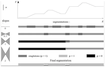
Figure 8: Function f is segmented by smooth path connections of increasing slopes. Then one takes at each point the largest class S with ∆f(S) ≤ c (from C. Ronse [12]).
7.2 Lasso
This algorithm, due to F. Zanoguera et Al. [18], appears also in [6]. An initial image has been segmented into α-flat zones, which generates a hierarchy as the slope α increases . The optimization consists then in drawing manually a closed curve around the object to segment. If A designates the inside of this lasso, then we take the following function
ω(S) = 0 when S ⊆ A ; S ∈ S (23)
ω(S) = 1 when not,
for energy, and we go from classes to partitions by ∨-composition of the energies. The largest cut that minimizes ω is depicted in Figure 9c. We see that the resulting contour follows the edges of the petals. Indeed, a segmented class can jump over this high gradient only for α large enough, and then this class is rejected because it spreads out beyond the limit of the lasso.
By taking a series {Aj, 1 ≤ j ≤ p} of increasing lassos Aj we make climbing the energy ω of Relation (23), and Theorem 12 applies. Unlike the previous case, where the λj are scalars numbers, the multiscale parametrization is now given by a family of increasing sets.
8
Conclusion
Other examples can be given, concerning colour imagery in particular [1]. At this stage, the main goal is to extend the above approach to vector data, and more generally to GIS type data.
Figure 9: a) Initial image; b) manual lasso; c) contour of the union of the classes inside the lasso.
References
[1] Angulo J., Serra, J., Modeling and segmentation of colour images in polar representations
Image and Vision Computing 25 (2007) 475-495.
[2] Benz´ecri J. P., L’Analyse des Donn´ees. Tome I : La Taxinomie. Dunod, Paris, 4`eme edition, 1984.
[3] Diday E., Lemaire J., Pouget J., Testu F., El´ements d’analyse des donn´ees .Dunod, Paris, 1982
[4] Guigues L., Cocquerez J.P., Le Men H., Scale-Sets Image Analysis, Int. Journal of
Computer Vision 68(3), 289-317, 2006.
[5] Guigues L., Mod`eles multi-´echelles pour la segmentation d’images.Th`ese doctorale Uni-versit´e de Cergy-Pontoise, d´ecembre 2003.
[6] Meyer F., Najman L. Segmentation, Minimum Spanning Trees, and Hierarchies, in
Math-ematical Morphology, L. Najman et H. Talbot, Eds. Wiley, N.Y. 2010.
[7] Mumford D. and Shah J., Boundary Detection by Minimizing Functionals, in Image
Understanding, S. Ulmann and W. Richards Eds, 1988.
[8] Najman L., and Schmitt M., Geodesic saliency of watershed contours and hierarchical segmentation. IEEE Trans. on PAMI, 18(12): 1163-1173, Dec. 1996
[9] Najman L.,Talbot H., Eds. Mathematical Morphology, Wiley, N.Y. 2010.
[10] Ronse, C., Partial partitions, partial connections and connective segmentation. Journal of Mathematical Imaging and Vision 32 (2008) 97–125
[11] Ronse, C., Idempotent block splitting on partial partitions, I: isotone operators, Order Vol. 28, no. 2 (2011), pp. 273-306.
[12] Ronse, C., Idempotent block splitting on partial partitions, II: non-isotone operators.
Order Vol. 28, no. 2 (2011), pp. 307-339.
[13] Salembier P., Garrido L., Binary Partition Tree as an Efficient Representation for Image Processing, Segmentation, and Information Retrieval. IEEE Trans. on Image Processing, 2000, 9(4): 561-576.
[14] Salembier P., Connected operators based on tree pruning strtegies, Chapter 7 in [9]. [15] Serra, J., Hierarchy and Optima, in Discrete Geometry for Computer Imagery, I.
Debled-Renneson et al.(Eds) LNCS 6007, Springer 2011, pp 35-46
[16] Soille, P., Constrained connectivity for hierarchical image partitioning and simplification. IEEE Transactions on Pattern Analysis and Machine Intelligence 30 (2008)1132–1145 [17] Soille, P., Grazzini, J. Constrained Connectivity and Transition Regions, in Mathematical
Morphlology and its Applications to Signal and Image Processing, M.H.F. Wilkinson and
B.T.M. Roerdink, Eds, Springer 2009, pp.59-70.
[18] Zanoguera, F., Marcotegui, B., Meyer, F. A toolbox for interactive segmentation based on nested partitions. In Proc. of ICIP’99 Kobe (Japan), 1999
![Figure 1: a) Basic input, b) and c) saliency maps from connected openings by dynamics [b)]](https://thumb-eu.123doks.com/thumbv2/123doknet/12402518.332169/3.892.187.734.185.430/figure-basic-input-saliency-maps-connected-openings-dynamics.webp)