Impacts of Packet Scheduling and Packet Loss Distribution on FEC Performances: Observations and Recommendations

(1)

HAL Id: inria-00000146

https://hal.inria.fr/inria-00000146

Submitted on 7 Jul 2005

HAL is a multi-disciplinary open access

archive for the deposit and dissemination of

sci-L’archive ouverte pluridisciplinaire HAL, est

destinée au dépôt et à la diffusion de documents

Distribution on FEC Performances: Observations and

Recommendations

Christoph Neumann, Vincent Roca, Aurelien Francillon, David Furodet

To cite this version:

Christoph Neumann, Vincent Roca, Aurelien Francillon, David Furodet. Impacts of Packet Scheduling

and Packet Loss Distribution on FEC Performances: Observations and Recommendations. [Research

Report] RR-5578, INRIA. 2005, pp.29. �inria-00000146�

(2)

a p p o r t

d e r e c h e r c h e

THÈME 1

Impacts of Packet Scheduling and Packet Loss

Distribution on FEC Performances: Observations

and Recommendations

Christoph NEUMANN

(1)

— Vincent ROCA

(1)

— Aurélien FRANCILLON

(1)

—

David FURODET

(2)

(1)

_{INRIA Rhône-Alpes, Planète Research Team - {firstname.name}@inrialpes.fr}

(2)

_{STMicroelectronics, AST, Grenoble, France - david.furodet@st.com}

N° 5578

(3)

(4)

Christoph NEUMANN

(1)

, Vincent ROCA

(1)

, Aurélien FRANCILLON

(1)

,

David FURODET

(2)

(1)

_{INRIA Rhône-Alpes, Planète Research Team - {firstname.name}@inrialpes.fr}

(2)

_{STMicroelectronics, AST, Grenoble, France - david.furodet@st.com}

Thème 1 — Réseaux et systèmes

Projet Planete

Rapport de recherche n° 5578 — Mai 2005 — 29 pages

Abstract: Forward Error Correction (FEC) is commonly used for content broadcasting. The

perfor-mance of the FEC codes largely vary, depending in particular on the object size and on the number of

parity packets produced, and these parameters have already been studied in detail by the community.

However the FEC performances are also largely dependent on the packet scheduling used during

transmission and on the loss pattern introduced by the channel. Therefore this work analyzes their

impacts on three FEC codes: LDGM Staircase, LDGM Triangle, two large block FEC codes, and

Reed-Solomon. Thanks to this analysis, we define several recommendations on how to best use these

codes, depending on the test case and on the channel, which turns out to be of utmost importance.

Key-words:

Multicast, Forward Error Correction (FEC), LDPC, Reed-Solomon, Loss Pattern,

Packet Scheduling

(5)

des Pertes de Paquets sur les Performances de trois Codes

Correcteurs d’Erreurs: Observations et Recommandations

Résumé : Les codes correcteurs d’erreurs (ou FEC, “Forward Error Correction”) sont largement

utillisés dans le contexte de la diffusion à large échelle de contenus. Les performances de ces codes

FEC dépendent fortement de la taille de l’objet encodé et du nombre de paquets de parité produits.

Ces deux paramètres ont déjà été étudiés en détails par la communauté. Toutefois les performances

dépendent aussi fortement de l’ordonnancement des paquets utilisé lors de la transmission ainsi que

de la distribution des pertes sur le canal de transmission. Par conséquent, ce travail analyse les

impacts de ces paramètres sur trois codes : LDGM Staircase et LDGM Triangle, deux codes FEC de

type grands blocs, et Reed-Solomon. Grace à cette analyse, nous établissons des recommandations

d’une très grande importance pratique pour une utilisation optimale de ces codes en fonction du

canal de transmission et du scénario d’utilisation.

Mots-clés : Multicast, Codes Correcteurs d’Erreurs, LDPC, Reed-Solomon, Distribution des Pertes

(6)

1 Introduction

1.1 Context of the work

This work analyzes the impacts of packet scheduling in the context of a content delivery systems like

”IP Datacast” (IPDC) [12, 6] in DVB-H, the ”Multimedia Broadcast/Multicast Service” (MBMS) [1]

in 3GPP, or data broadcast to cars (e.g. [5]). These systems are characterized by the fact that there

is no back channel, and therefore no repeat request mechanism can be used that would enable the

source to adapt its transmission according to the feedback information sent by the receiver(s). The

lack of feedback channel however enables an unlimited scalability in terms of number of receivers,

who behave in a completely asynchronous way. Using a reliable multicast transmission protocol like

ALC [9], along with the FLUTE [13] file delivery application, can turn out to be highly effective in

this context [5].

Yet, in order to be efficient, these approaches largely rely on the use of a Forward Error

Correc-tion (FEC) scheme running at the applicaCorrec-tion layer, within the ALC reliable transport protocol (we

motivate the use of FEC in section 4.2). The channel is therefore a “packet erasure channel” and

packets either arrive (with no error) or are lost (e.g. because of router congestion problems). After

an FEC encoding of the content, redundant data is transmitted along with the original data. Thanks

to this redundancy, up to a certain number of missing packets can be recovered at the receiver. The

great advantage of using FEC with multicast or broadcast transmissions is that the same parity packet

can recover different lost packets at different receivers.

Since we only consider file delivery applications in this work, the transmission latency has little

importance, which would not be true with streaming applications. Therefore we will not consider

the potential impacts of FEC codes and transmission scheme on the decoding latency at a receiver.

1.2 Goals of the work

The performance of the FEC code is largely impacted by the transmission scheduling. For instance,

sending all source packets first and then parity packets does not necessarily yield the same efficiency

as sending the packets in random order. The packet loss distribution observed by a receiver also

largely impact the decoding performances and a given transmission scheme may yield good results

for a specific loss distribution and yield catastrophic results in other circumstances. This work

ana-lyzes the impacts of packet scheduling and loss behaviors on the performances of three FEC codes:

Reed-Solomon, LDGM Staircase and LDGM Triangle. Thanks to this analysis, we define several

recommendations on how to best use these codes, which turns out to be of utmost practical

impor-tance. For instance it enables to optimize the FLUTE session to a specific download environment, or

on the opposite, to find transmission schemes that will behave correctly (but may be not optimally)

in a wide set of different environments.

In this work we do not considered FEC codes who are known to be covered by IPRs and for

which no public domain, open-source, implementation exists. In particular we will not consider

Tornado™ and Raptor™ codes [4]. This deliberate choice is likely to enlarge the usefulness of our

results to a large part of the community who prefer free codes.

(7)

The remainder of the paper is organized as follows: we first introduce the three FEC codes;

section 3 explains and motivates the modeling method we used; section 4 presents and analyzes the

performance of several transmission schemes while section 5 does the same with a reception model;

finally section 6 explains how to use these results in practice, then we conclude.

2 Introduction to RSE, LDGM Staircase and LDGM Triangle

Codes

2.1 Terminology

FEC encoding of an object produces redundant data. Thanks to this redundancy, up to a certain

number of missing packets can be recovered at the receiver. More precisely

k source packets (A.K.A.

data packets) are encoded into

n packets (A.K.A. encoding packets). The additional n − k packets

are called parity packets (A.K.A. FEC or redundancy packets). A receiver can then recover the

k

source packets provided it receives any

k packets (or a little bit more than k with LDGM/LDPC

codes) out of the

n possible. The FEC expansion ratio is the

n

k

ratio and it defines the amount of

parity packets produced. It is the inverse of the code rate (i.e.

k

_n

). In the present paper we will only

consider the FEC expansion ratio terminology.

2.2 RSE Code

The Reed-Solomon erasure code (RSE) is one of the most popular FEC codes. RSE is intrinsically

limited by the Galois Field it uses [14]. A typical example is GF(

2

8 ) where

n ≤ 256. With one

kilobyte packets, a FEC codec producing as many parity packets as data packets (i.e.

n = 2k)

operates on blocks of size

128 kilobytes at most, and all files exceeding this threshold must be

segmented into several blocks, which reduces the global packet erasure recovery efficiency (e.g. if

B blocks are required, a given parity packet has a probability 1/B to recover a given erasure, and

B = 1 is then the optimal solution). This phenomenon is known as the “Coupon Collector Problem”

[3]. Another drawback is a huge encoding/decoding time with large

(k, n) values, which is the

reason why GF(

2

8 ) is preferred to GF(

2

16 ) in spite of its limitations on the block size. Yet RSE is

optimal (it is an MDS code) because a receiver can recover erasures as soon as it has received exactly

k packets out of n for a given block.

2.3 LDGM Codes

We now consider another class of FEC codes that completely departs from RSE: Low Density

Gener-ator Matrix (LDGM) codes, that are variants of the well known LDPC codes introduced by Gallager

in the 1960s [7].

(8)

p_7

p_9

p_8

s_1

s_5

s_4

s_3

s_2

s_6

source

nodes

k

n − k

parity

nodes

c1: s_2 + s_4 + s_5 + s_6 + p_7 = 0

c2: s_1 + s_2 + s_3 + s_6 + p_8 = 0

c3: s_1 + s_3 + s_4 + s_5 + p_9 = 0

(n) Message Nodes

(n − k) Check Nodes

(a) Bipartite graph

s

1

0

1

0

1

0

1

0

1

0

1

6

7 p

s

9 ...

...

c

1 c

2 c

3

3 Id

1

0 [ H |

] =

p

1 (b) H matrix

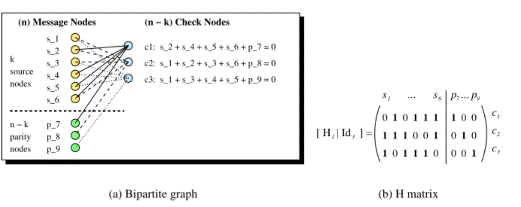
Figure 1: A regular bipartite graph and its associated parity check matrix for LDGM.

2.3.1 Principles

LDGM codes rely on a bipartite graph between left nodes, called message nodes, and right nodes,

called check nodes (A.K.A. constraint nodes). The

k source packets form the first k message nodes,

while the parity packets form the remaining

n − k message nodes. The upper part of this graph

is built following an appropriate left and right degree distribution (in our work the left degree is

3).

The lower part of this graph follows other rules that depend on the variant of LDGM considered (e.g.

with LDGM, figure 1 (a), there is a bijection between parity and check nodes). This graph creates a

system of

n − k linear equations (one per check node) of n variables (source and parity packets).

A dual representation consists in building a parity check matrix,

H. With LDGM, this matrix is

the concatenation of matrix

H

1 and an identity matrix

I

_n−k

. There is a

1 in the {i; j} entry of matrix

H each time there is an edge between message node j and check node i in the associated bipartite

graph.

Thanks to this structure, encoding is extremely fast: each parity packet is equal to the sum of

all source packets in the associated equation. For instance, packet

p

7 is equal to the sum:

s

2 ⊕

s

4 ⊕ s

5 ⊕ s

6 . Besides LDPC/LDGM codes can operate on very large blocks: several hundreds of

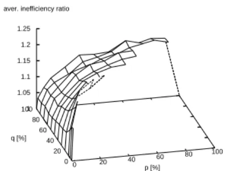
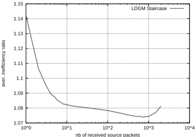
MBytes are common. However LDGM is not an MDS code and it introduces a decoding inefficiency:

inef _ratio ∗ k packets, with inef _ratio ≥ 1, must be received for decoding to be successful. The

inef _ratio, experimentally evaluated, is therefore a key performance metric.

2.3.2 Iterative Decoding Algorithm

With LDGM, there is no way to know in advance how many packets must be received before

de-coding is successful (LDGM is not an MDS code). Dede-coding is performed step by step, after each

packet arrival, and may be stopped at any time.

The algorithm is simple: we have a set of

n − k linear equations of n variables (source and parity

packets). As such this system cannot be solved and we need to receive packets from the network.

Each non duplicated incoming packet contains the value of the associated variable, so we replace this

(9)

variable in all linear equations in which it appears. If one of the equations has only one remaining

unknown variable, then its value is that of the constant term. We then replace this variable by its

value in all remaining equations and reiterate, recursively. As we approach the end of decoding,

incoming packets tend to trigger the decoding of several packets, until all of the

k source packets

have been recovered.

2.3.3 LDGM Staircase Code

This trivial variant, suggested in [10], only differs from LDGM by the fact that the

I

n−k

matrix is

re-placed by a “staircase matrix” of the same size. This small variation affects neither encoding, which

remains a simple and highly efficient process, nor decoding, which follows the same algorithm. But

this simple variation largely improves the FEC code efficiency.

2.3.4 LDGM Triangle Code

In this variant of LDGM Staircase, the triangle beneath the staircase diagonal is now filled, following

an appropriate rule [15]. This rule adds a “progressive” dependency between check nodes, as shown

in figure 2. This variation further increases performance in some situations, while keeping encoding

highly efficient (even if a bit slower since there are more "1"s per row). Here also decoding follows

the same iterative algorithm.

Interested readers are invited to refer to [15]. An open source, GNU/LGPL implementation of

these codes is also available at [11].

1 1 1 1 1 1 1 1 1 1 1 1 1 1 11 1 1 1 1 1 1 1 1 1 1 1 1 11 1 1 1 1 1 1 1 1 1 1 1 1 1 1 1 1 1 1 1 1 1 1 1 1 1 1 1 1 1 1 1 1 1 1 1 1 1 1 1 1 1 1 1 1 1 1 1 1 1 1 1 1 1 1 1 11 1 1 1 1 1 1 1 1 1 1 1 1 1 1 11 1 1 1 1 1 1 1 1 1 1 1 1 1 1 1 1 11 1 1 1 1 1 1 1 1 1 1 1 1 1 1 1 1 1 1 1 1 1 1 1 1 1 1 1 1 1 1 1 1 1 1 1 1 1 1 1 1 1 1 1 1 1 1 1 1 1 1 1 1 1 1 1 1 1 1 1 1 1 1 1 1 1 1 1 1 1 1 1 1 1 1 1 1 11 1 1 1 1 1 1 1 1 11 1 1 1 1 1 1 1 1 1 1 1 1 1 1 1 1 1 1 1 1 1 1 1 1 1 1 1 1 1 1 1 1 1 1 1 1 1 1 1 1 1 1 1 1 1 1 1 1 1 1 1 1 1 1 1 1 1 1 1 1 1 1 1 1 1 1 1 1 1 1 1 1 1 1 1 1 1 1 1 1 1 1 1 1 1 1 1 1 1 1 1 1 1 1 1 1 1 1 1 1 1 1 1 1 1 1 1 1 1 1 1 1 1 1 1 1 1 1 1 1 1 1 1 1 1 1 1 1 1 1 1 1 1 1 1 1 1 1 11 1 11 1 1 1 1 1 1 1 1 1 1 1 1 1 1 1 1 1 1 1 1 1 1 1 1 1 1 1 1 1 1 1 1 1 1 1 1 1 1 1 1 1 1 1 1 1 1 1 1 1 1 1 1 1 1 1 1 1 1 1 11 1 1 1 1 1 1 1 1 1 1 1 1 1 1 1 1 1 1 1 1 1 1 1 1 1 1 1 1 1 1 1 1 1 1 1 1 1 1 1 1 1 1 1 1 1 1 1 1 1 1 1 1 1 1 1 1 1 1 1 1 1 1 1 1 1 1 1 1 1 1 1 1 1 1 1 1 11 1 1 1 1 1 1 1 1 1 1 1 1 1 1 1 1 1 1 1 1 1 1 1 1 1 1 1 11 1 1 1 1 1 1 1 1 1 1 1 1 1 11 1 1 1 1 111 1 1 1 1 1 11 1 1 1 1 1 111 1 1 1 1111 1 1 1 1 1 11 1 1 1 1 11 1 1 1 11 11 1 1 1 1 1 1 11 1 1 1 1 1 11 111 1 1 1 1 1 1 11 11 1 1 1 11 1 11 1 1 1 1 11 1 1 1 1 1 11 1 1 1 1 1 1 11 1 1 1 1 1 11 1 1 1 1 1 11 1 1 1 1 1 11 1 1 1 1 1 1 11 1 1 1 1 1 1 1 11 1 1 1 1 11 1 1 1 1 11 1 11 1 1 1 1 1 11 11 1 1 1 1 1 1 11 1 1 1 1 1 1 11 1 1 1 1 1 1 11 1 1 1 1 1 1 11 1 1 1 1 1 1 11 1 1 1 1 1 1 1 1 11 1 1 1 1 1 1 11 1 1 1 1 1 1 1 1 11 11 1 1 1 1 1 11 1 1 11 1 1 1 1 1 11 1 1 1 1 1 1 11 1 1 1 1 1 1 1 11 1 1 1 1 1 1 11 1 1 1 1 1 1 1 11 1 1 1 1 1 111 11 1 1 1 1 1 1 1 11 1 1 1 1 1 1 1 1 11 1 1 1 1 11 1 1 1 1 11 1 1 1 1 1 1 1 11 1 1 1 1 1 1 1 1 11 1 1 1 1 11 1 1 1 1 1 1 1 11 1 1 1 1 1 1 11 1 1 1 1 1 1 1 11 1 1 1 1 1 1 11 1 1 1 1 1 1 1 11 1 1 1 1 1 11 11 1 1 1 1 1 1 1 1 11 1 1 1 1 1 1 11 1 1 1 1 1 1 1 1 1 1 11 1 1 1 1 1 1 11 1 1 1 1 1 1 1 1 11 1 1 1 1 1 1 1 11 1 1 1 1 1 1 11 1 1 1 1 1 1 1 1 1 11 1 1 1 1 1 1 11 1 1 1 11 1 11 1 1 1 1 1 1 11 1 1 1 1 1 1 11 1 1 1 1 1 1 11 1 1 1 1 11 1 1 11 1 1 1 1 1 1 1 11 1 1 1 1 1 1 1 1 11 1 1 1 1 1 11 1 1 1 1 1 1 1 11 1 1 1 1 1 1 1 1 11 1 1 1 1 1 11 1 1 1 1 1 1 11 11 1 1 1 1 1 1 11 11 1 1 1 1 1 1 1 11 1 1 1 1 1 1 11 11 1 1 1 1 1 1 1 1 1 1 11 1 1 1 11 11 1 1 1 1 1 11 1 1 1 1 1 1 1 11 1 1 1 1 1 1 1 1 1 11 1 1 1 1 1 11 1 1 1 11 1 11 1 1 1 1 1 1 1 11 1 1 1 1 11 11 1 1 1 1 11 1 11 1 1 1 1 1 1 11 1 1 1 1 11 1 11 1 1 1 1 1 1 1 11 1 1 1 1 1 1 1 11 1 1 1 1 1 1 1 11 1 1 1 11 1 11 1 1 1 11 1 11 1 1 1 1 1 1 1 1 11 11 1 1 1 1 11 1 1 1 1 1 1 1 1 11 1 1 1 1 1 1 11 1 1 1 1 1 1 1 11 1 1 1 1 1 11 1 1 1 11 1 1 1 1 1 1 1 1 11 1 1 1 1 1 1 11 1 1 1 1 1 1 1 1 11 1 1 1 1 1 1 11 1 1 1 1 1 1 1 11 1 1 1 1 1 1 1 1 1 11 1 1 1 1 11 1 1 1 11 1 1 1 1 1 1 1 11 1 1 1 1 1 1 11 1 1 1 1 1 1 1 11 1 1 1 1 1 1 1 11 1 1 1 1 1 11 1 111 1 1 1 1 1 1 1 1 11 1 1 1 1 1 1 11 1 1 1 1 1 1 1 11 1 1 1 1 1 1 1 1 11 1 1 1 1 11 1 1 1 1 1 1 11 1 1 1 1 11 1 1 11 1 1 1 1 1 1 1 1 1 11 1 1 1 1 1 1 11 1 1 11 1 1 1 1 1 1 1 1 1 11 1 1 1 1 1 1 11 1 1 1 1 1 11 1 11 1 11 1 1 1 1 11 11 1 1 1 1 1 1 11 1 1 1 1 1 1 1 1 11 1 1 1 1 1 1 11 1 1 1 1 11 1 1 1 1 1 11 1 11 1 1 1 1 1 1 1 11 1 1 1 1 1 1 1 1 11 1 1 1 1 1 1 1 1 11 1 1 1 1 1 1 1 1 1 11 1 1 1 1 1 1 1 1 1 1 111 1 1 1 1 111 1 1 1 11 1 1 1 1 1 1 1 1 1 1 11 1 1 1 1 1 1 11 1 1 1 1 1 1 11 1 1 1 1 1 1 1 1 11 11 1 1 1 1 1 1 11 1 1 1 1 1 111 1 1 1 1 11 1 1 1 1 1 1 1 1 1 1 11 1 1 1 1 11 11 1 1 11 1 1 1 1 1 1 1 11 1 1 1 1 1 1 1 1 1 11 1 1 1 1 1 1 1 1 1 11 1 1 1 1 1 1 1 11 1 1 1 1 11 1 111 1 1 1 1 1 1 1 1 11 1 1 1 1 1 1 11 1 1 1 1 1 1 1 1 1 11 1 1 1 1 1 11 1 1 11 1 1 1 1 1 1 1 1 11 1 1 1 1 1 1 1 1 11 1 1 1 1 1 1 11 1 1 1 1 11 1 1 1 1 1 11 1 1 1 1 1 1 1 1 1 11 1 1 1 1 1 1 1 1 1 1 1 11 1 1 1 1 1 11 1 1 1 1 1 1 1 1 1 11 1 1 1 1 1 1 1 1 1 1 11 1 1 1 1 1 1 1 1 1 11 1 1 1 1 1 1 11 1 1 1 1 1 1 1 1 11 1 1 1 1 1 11 1 1 11 1 1 1 1 1 1 1 1 11 1 1 1 1 1 1 1 11 1 1 11 1 11 1 1 11 1 1 1 11 1 1 1 1 1 1 11 1 1 1 1 1 11 1 1 1 1 1 1 1 1 11 1 1 1 1 1 1 1 1 1 11 1 1 1 1 1 1 1 1 11 1 1 1 1 1 1 11 1 1 1 1 1 1 1 11 1 1 1 1 1 1 1 1 1 1 1 1 11 1 1 1 1 1 1 1 11 1 1 1 1 1 1 1 11 1 1 1 1 11 1 1 11 1 1 1 1 1 1 1 11 1 1 1 1 1 1 1 1 11 1 1 1 1 1 1 1 1 1 1 1 11 1 1 1 1 1 1 1 1 1 1 11 11 1 1 1 1 1 1 1 1 11 1 1 1 1 1 1 1 1 1 1 1 11 1 1 1 1 1 11 1 1 1 11 1 1 1 1 1 1 1 11 1 1 1 1 1 1 1 1 1 1 11 1 1 1 1 1 1 1 1 1 11 1 1 1 1 1 1 11 1 1 1 1 1 11 1 1 1 1 1 1 1 1 11 1 1 1 1 1 1 1 1 1 11 1 1 1 1 1 1 1 1 11 1 1 1 1 1 1 1 1 1 1 11 1 1 1 1 1 1 1 1 1 11 1 1 1 1 1 1 11 11 1 1 1 1 1 1 1 1 11 1 1 1 1 1 11

(10)

3 Modeling of the Whole System

3.1 The Three Models

Let’s imagine that a server wants to broadcast a big file using a large scale content delivery system

using FLUTE. The content is first FEC encoded which produces additional parity packets (we

mo-tivate the use of FEC in section 4.2). The sender must now decide in which order source and parity

packets will be sent, and this choice will largely impact the whole system performances as we will

see later. This packet scheduling constitutes the transmission model.

The channel is characterized by a packet loss distribution. It may be a lossy channel with long

bursts of packet erasures, or it may be a channel where losses are completely independent from one

another. This packet loss distribution constitutes the loss model.

channel

transmission

scheduling

Reality

Model

_model

reception

model

transmission

loss model

FEC code

+

Figure 3: Modeling methods.

These two transmission and loss models together characterize a reception behavior at a receiver

(Figure 3). In case of broadcast applications, there is no reason that different receivers experience

the same loss model, so the reception behavior is receiver dependent. This is the approach that will

be used for most experimental evaluations (section 4).

The reception behavior may also be modeled the other way round, by providing a reception

model. This model defines which packets are received (and when) by a receiver. This approach can

be complementary to the use of the transmission and loss models, for instance to study the FEC code

performances in controlled situations. This is the approach that will be used in section 5.

3.2 The Channel Model

Finding an appropriate error model for a given channel is a complex task, especially with wireless

networks where it is difficult to take into account all parameters (e.g. channel fading, reflections,

refractions, diffractions, Doppler effects). Yet in this work we are only interested in a packet loss

model (rather than a bit error model) that provides a high level abstraction of the channel parameters.

The well known two state Markov model (A.K.A. Gilbert model) is such a simplified loss model,

and it is widely used in the literature [2, 16].

The model is composed of two states: the no-loss state where no packet loss occurs, and the loss

state where packets are lost (figure 4).

p indicates the probability to go from no-loss state to loss

(11)

q

loss

no loss

p

1 − p

1 − q

Figure 4: Two state Markov loss model.

probability [2]:

p

global

=

p

p + q

This probability is represented as a 3D-graph in figure 5.

0

0.2

0.4

0.6

0.8

1

0

0.2

0.4

0.6

0.8

1

0

0.2

0.4

0.6

0.8

1 global packet loss probabilty

p

q

global packet loss probabilty

Figure 5: Global loss probability.

Depending on the channel modeled, the

p and q values will differ. For a given channel it may

be possible to determine

p and q using packet loss traces. For instance, this has been done in [8] for

traces coming from an GSM channel, and in [16] for traces coming from end-to-end connections in

the Internet.

The Gilbert model also covers some specific loss behaviors that we want to emphasize:

• No loss: This perfect channel corresponds to

p = 0.

• Independent and Identically Distributed (IID) losses (A.K.A. the Bernoulli model): This

mem-oryless channel corresponds to

q = 1 − p.

(12)

We are aware that the Gilbert model has some shortcomings in error modeling accuracy [8, 16].

We believe that it is however sufficient for our work since it already covers a very large set of loss

behaviors. Moreover we took care to perform experiments with a very large set of

p and q values

(

14 × 14 grid) in order to cover as many channel behaviors as possible. Other more complex models

(e.g. the n-state Markov models), that may be required for specific channels, will be considered in

future works.

When is Decoding Impossible?

In our work we want to know, given a certain FEC code, how many losses a receiver can support.

With the Gilbert model we can calculate the maximum number of packet losses supported by any

FEC code. Let’s consider a FEC code producing

n−k parity packets from k source packets. We then

transmit

n

sent

≤ n packets over the network (sending all packets is not mandatory, see section 5).

The number of packets actually received is equal to:

n

received

= n

sent

∗ (1 − p

global

)

(1)

n

received

must be at least equal to

inef _ratio ∗ k (remember that LDGM codes are not MDS) for

decoding to be successful. When

n

received

= inef _ratio ∗ k we have:

q =

−p ∗ inef _ratio

inef _ratio −

n

sent

k

These limits are shown in figure 6 for FEC expansion ratios 1.5 and 2.5, and assuming

inef _ratio =

1 (which is a lower bound for inef _ratio). This figure shows that several areas of the (p, q)

pa-rameter space cannot enable a receiver to decode the object. This is not a flaw of the FEC code, it’s

merely a fundamental limitation.

000000000000000000

111111111111111111

Decoding impossible (number

of packets received < k):

00000000000000000

11111111111111111

00

11

00

11

11 Totally uncorrelated losses

0

0.2

0.4

0.6

0.8

1

0

0.2

0.4

0.6

0.8

1 p

FEC expansion ratio = 2.5

FEC expansion ratio = 1.5

q

No/very few loss

High loss rate, no bursts

High loss rate, in bursts

(13)

4 Simulation Results With Six Transmission Models

4.1 Methodology

The methodology used to conduct performance tests is the following. We considered the RSE,

LDGM Staircase and LDGM Triangle codes, and two typical FEC expansion ratios: 1.5 and 2.5

(they correspond to code rates

2/3 and 2/5 respectively). The object is composed of 20000 packets

(i.e.

k = 20000 with LDGM-* codes).

The performance metric used is the average inefficiency ratio:

inef _ratio =

n

necessary

_

f or

_

decoding

k

,

which is the total number of packets received when decoding completes, divided by the number of

source packets. Of course the optimal value is

1.0, and the higher this inef _ratio, the more packets

are needed in excess to

k for decoding, which is not good

1 _.

We considered six different transmission models. Although this is not an exhaustive study, we

believe that these transmission schemes already cover a large set of possibilities and give good

insights on the overall performances.

For each transmission model and FEC code, we study the impacts of the channel by varying the

p and q probabilities in [0; 1] (14 × 14 values are considered for (p; q)). Each point in the resulting

3-D graphs is the average

inef _ratio value over 100 simulations. Yet if decoding fails for any of

the

100 tests, we do not plot any point. This strict strategy enables us to better highlight the areas

where the decoding probability is not acceptable. The numerical results of our simulation for the

most interesting transmission schemes and codes are reported in the Appendix of this paper.

For comparison purposes, we sometimes plot an additional curve,

n

received

k

, which corresponds

to the total number of packets received (even after decoding stopped) divided by the number of

source packets. This is the maximum value that the inefficiency ratio can achieve. It also gives

an idea on the number of packets that a receiver may still receive after decoding (

n

received

−

n

necessary

_

f or

_

decoding

). When

n

received

_k

= 1 the curve corresponds to the limits described in

section 3.2 and figure 6. Any additional packet loss will necessarily lead decoding to fail.

4.2 Why is FEC Needed?

To motivate the use of FEC, we did a small test. Rather than using FEC to recover losses, a sender

may decide to transmit each packet

x times. In figure 7 x = 2 and packets are sent in a random

order. It shows that decoding is only possible with

p = 0, and the average inefficiency ratio is then

near

2.0 which means that the receiver waits almost systematically the end of the transmission to

reconstruct the object. For all

p > 0 at least one experiment failed, and therefore no inefficiency

ratio is shown, as explained in section 4.1. This test highlights the poor performances when using

repetition only instead of FEC for content broadcasting.

1 _{With large block LDGM codes, an inefficiency ratio greater than}

₁

.0 is caused by the non MDS nature of these codes,

whereas with RSE, which is an MDS code, this is caused by the coupon collector problem (section 2.2). More information

can be found in [15].

(14)

0

1

2

3

4 5 0

20

40

60

80

100

1

1.2

1.4

1.6

1.8

2 aver. inefficiency ratio

No FEC inefficiency ratio

p [%]

q [%]

aver. inefficiency ratio

Figure 7: Performances without FEC but

2 repetitions.

4.3 Tx_model_1: Send Source Packets Sequentially, Then Parity Packets

This scheme consists in sending all source packets sequentially, and then all parity packets, also

sequentially. The results are shown in figure 8 (the LDGM Staircase curves are not shown since

results are similar to LDGM Triangle).

We notice a first obvious result: without loss (

p = 0) the inefficiency ratio is 1.0 with all codes.

Indeed, all source packets are received and the receiver does not need any of the following parity

packets. We’ll see that other transmission schemes do not necessarily have this good property.

With losses (in burst or not) all codes show a similar behavior. The inefficiency ratio curve is

very close to the

n

received

k

curve for nearly all values of

p and q. It means that the receiver always

needs to wait almost the end of transmission to reconstruct the object. With RSE this is not surprising

since the object is segmented in blocks: if a source packet of the last block is lost, the receiver needs

to wait the end of the transmission, when the associated parity packets will be sent.

With LDGM codes this behavior is more surprising. These large block FEC codes encode the

whole object directly, and parity packets are created using source packets coming from different parts

of the content. However each parity packet depends on the previous one (because of the staircase in

the parity check matrix, also present in LDGM Triangle codes). This dependency negatively impacts

decoding performance when several sequential parity packets get lost.

Finally, RSE covers a smaller area (when

z − axis > 0) than LDGM-* codes, which indicates

that its erasure recovery capabilities are more limited. This is especially true for long packet loss

bursts (small

q). This is easy to understand: since packets are sent sequentially, and a single long

burst results in the loss of a large number of packets of the same block. Decoding this block becomes

difficult, especially with a small FEC expansion ratio (e.g.

1.5).

(15)

0

20

40

60

80 100 0

20

40

60

80

100

1

1.2

1.4

1.6

1.8

2

2.2

2.4 aver. inefficiency ratio

RSE inefficiency ratio

n

received

/k

p [%]

q [%]

aver. inefficiency ratio

(a) RSE and a FEC expansion ratio of 2.5.

0

20

40

60

80 100 0

20

40

60

80

100

1

1.2

1.4

1.6

1.8

2

2.2

2.4 aver. inefficiency ratio

LDGM Triangle inefficiency ratio

n

received

/k

p [%]

q [%]

aver. inefficiency ratio

(b) LDGM Triangle and a FEC expansion ratio of 2.5.

0

20

40

60

80 100 0

20

40

60

80

100

1

1.1

1.2

1.3

1.4

1.5 aver. inefficiency ratio

RSE inefficiency ratio

n

received

/k

p [%]

q [%]

aver. inefficiency ratio

(c) RSE and a FEC expansion ratio of 1.5.

0

20

40

60

80 100 0

20

40

60

80

100

1

1.1

1.2

1.3

1.4

1.5 aver. inefficiency ratio

LDGM Triangle inefficiency ratio

n

received

/k

p [%]

q [%]

aver. inefficiency ratio

(d) LDGM Triangle and a FEC expansion ratio of 1.5.

Figure 8: Tx_model_1

4.4 Tx_model_2: Send Source Packets Sequentially, Then Parity Packets

Ran-domly

One idea to counteract the bad results of Tx_model_1 is to transmit the parity packets in a random

order rather than sequentially. For RSE the advantage is clear: parity packets of the last few blocks

can be transmitted earlier, so the receiver has on average less to wait before receiving parity packets

for any block. This is confirmed in figures 9(a) and 9(c). The inefficiency ratio is much better than

with Tx_model_1 and moreover this ratio is relatively constant.

LDGM Triangle codes exhibit relatively good performances and largely outperform RSE codes

(figures 9(b) and 9(d)). Yet the LDGM Staircase 3D-curve has a hole around

p = 50 and q =

(16)

70 (Figure 9(b)), where exactly one test failed. This is not acceptable in practice, and therefore

Tx_model_2 is not recommended with LDGM Staircase and higher loss ratios. Conversely LDGM

Staircase may be used with small loss ratios where the code yields very good results.

This transmission model confirms that with LDGM-* codes, parity packets should not be sent

sequentially but randomly, to prevent the loss of sequences of parity packets. All the following tests

will confirm this observation.

RSE

LDGM Staircase

0

20

40

60

80

100 p [%]

₀

20

40

60

80

100 q [%]

1

1.1

1.2

1.3

1.4

1.5 aver. inefficiency ratio

(a) RSE versus LDGM Staircase and a FEC

expan-sion ratio of 2.5.

LDGM Staircase

LDGM Triangle

0

20

40

60

80

100 p [%]

₀

20

40

60

80

100 q [%]

1

1.02

1.04

1.06

1.08

1.1

1.12

1.14

1.16

1.18

1.2 aver. inefficiency ratio

(b) LDGM Triangle vs. Staircase and a FEC

expan-sion ratio of 2.5.

RSE

LDGM Staircase

0

20

40

60

80

100 p [%]

₀

20

40

60

80

100 q [%]

1

1.02

1.04

1.06

1.08

1.1

1.12

1.14

1.16

1.18

1.2 aver. inefficiency ratio

(c) RSE versus LDGM Staircase and a FEC

expan-sion ratio of 1.5.

LDGM Staircase

LDGM Triangle

0

20

40

60

80

100 p [%]

₀

20

40

60

80

100 q [%]

1

1.02

1.04

1.06

1.08

1.1 aver. inefficiency ratio

(d) LDGM Triangle vs. Staircase and a FEC

expan-sion ratio of 1.5.

(17)

4.5 Tx_model_3: Send Parity Packets Sequentially, Then Source Packets

Ran-domly

We now consider the case dual to Tx_model_2: we first transmit all parity packets sequentially, then

we transmit the source packets either sequentially or randomly. We only consider the latter case in

this paper since tests (not included in this paper) have shown that sending the source packets

sequen-tially yields uninteresting results (it makes no difference with LDGM-* codes, and we experience a

worse behavior with RSE).

Non-systematic FEC codes can decode using only parity packets (no source packet). RSE can

be used as a non-systematic code if the number parity packets is high enough (i.e. if

n − k ≥ k).

But this is not the case with LDGM Triangle and Staircase that need at least a small number of data

packets to start decoding.

Figure 10 shows that with

p = 0, the LDGM-* codes need exactly one source packet to decode

the content, and therefore the inefficiency ratio is

≈ 1.5 for a FEC expansion ratio of 2.5. With RSE,

the receiver needs

29903 packets when p = 0, that is to say decoding is possible when k packets of

the last block have been received. Therefore the inefficiency ratio is also

≈ 1.5 for a FEC expansion

ratio of

2.5. Globally, these tests show that performances are not that interesting, and this transmission scheme

may only be interesting for some specific loss patterns.

(18)

0

20

40

60

80 100 0

20

40

60

80

100

1

1.1

1.2

1.3

1.4

1.5 aver. inefficiency ratio

RSE inefficiency ratio

n

received

/k

p [%]

q [%]

aver. inefficiency ratio

(a) RSE and a FEC expansion ratio of 2.5.

0

20

40

60

80 100 0

20

40

60

80

100

1

1.1

1.2

1.3

1.4

1.5 aver. inefficiency ratio

LDGM Staircase inefficiency ratio

n

received

/k

p [%]

q [%]

aver. inefficiency ratio

(b) LDGM Staircase and a FEC expansion ratio of

2.5.

0

20

40

60

80 100 0

20

40

60

80

100

1

1.1

1.2

1.3

1.4

1.5 aver. inefficiency ratio

LDGM Staircase inefficiency ratio

n

received

/k

p [%]

q [%]

aver. inefficiency ratio

(c) LDGM Triangle and a FEC expansion ratio of 2.5.

0

20

40

60

80 100 0

20

40

60

80

100

1

1.02

1.04

1.06

1.08

1.1

1.12

1.14

1.16

1.18

1.2 aver. inefficiency ratio

RSE inefficiency ratio

n

received

/k

p [%]

q [%]

aver. inefficiency ratio

(d) RSE and a FEC expansion ratio of 1.5.

0

20

40

60

80 100 0

20

40

60

80

100

1

1.02

1.04

1.06

1.08

1.1 aver. inefficiency ratio

LDGM Staircase inefficiency ratio

n

received

/k

p [%]

q [%]

aver. inefficiency ratio

(e) LDGM Staircase and a FEC expansion ratio of

0

20

40

60

80 100 0

20

40

60

80

100

1

1.02

1.04

1.06

1.08

1.1 aver. inefficiency ratio

LDGM Triangle inefficiency ratio

n

received

/k

p [%]

q [%]

aver. inefficiency ratio

(19)

4.6 Tx_model_4: Send Everything Randomly

In this transmission model, source and parity packets are sent in a fully random order.

Results are shown in figure 11. RSE offers the worst performances with an inefficiency ratio

around

1.25. LDGM Staircase performs better and offers a ratio of 1.15. Finally LDGM Triangle

yields the best results with ratios going from

1.12 to 1.14.

For the RSE and LDGM Staircase codes, the performances are relatively stable, independently

of the packet loss behavior. This is not true with LDGM Triangle codes, that show better results

with smaller

p

global

. This observation can generally be made when LDGM Triangle sends it parity

packets randomly: it achieves better inefficiency ratios with smaller

p

global

. On the opposite, LDGM

Staircase codes are not sensitive to

p

global

in this case.

4.7 Tx_model_5: Interleaving (RSE only)

Packet interleaving is a commonly used solution with small block FEC codes like RSE to increase

their robustness against packet erasure bursts. The idea is to spread the transmission of one block

over an interval that is longer that the loss burst duration. The maximum distance between two packet

transmissions of the same block is achieved by sending successively one packet of each block, until

reaching the last block, and then continuing with the following packet of each block, and so on.

With LDGM codes this interleaving scheme is not feasible since there is only one block. What

we call interleaving for LDGM consists in sending successively one source packet and

n

_k

parity

packet (because the FEC expansion ratio is not necessarily equal to

2), and so one.

Results are shown in figure 12. As suspected, results are excellent with RSE, actually the best

ones compared to all other transmission schemes. The packets are optimally aligned using

interleav-ing, and for all loss patterns this solution give optimal results. This is not a surprise since interleaving

has been intensively used along with RSE codes.

4.8 Tx_model_6: Send Randomly a Few Source Packets Plus Parity Packets

In this transmission model we transmit only a few source packets in addition to all parity

pack-ets. More precisely, we first pick randomly

20% source packets and schedule them randomly with

all parity packets. This transmission model requires that the FEC expansion ratio be high enough

(otherwise less than

k packets will be received), and we chose 2.5.

The results are shown in figure 13. If all codes have constant performances, LDGM Staircase

largely outperform other codes. Note that the fact that LDGM Staircase performs better than Triangle

is rather unusual.

5 Simulation Results With a Reception Model

In this section we directly specify a reception model, without any consideration for the transmission

and loss models that may generate it. The goal is to better analyze an FEC code performances in a

completely controlled environment.

(20)

RSE

LDGM Staircase

0

20

40

60

80

100 p [%]

₀

20

40

60

80

100 q [%]

1

1.05

1.1

1.15

1.2

1.25

1.3 aver. inefficiency ratio

(a) RSE versus LDGM Staircase and a FEC

expan-sion ratio of 2.5.

LDGM Staircase

LDGM Triangle

0

20

40

60

80

100 p [%]

₀

20

40

60

80

100 q [%]

1.1

1.11

1.12

1.13

1.14

1.15

1.16 aver. inefficiency ratio

(b) LDGM Triangle vs. Staircase and a FEC

expan-sion ratio of 2.5.

RSE

LDGM Staircase

0

20

40

60

80

100 p [%]

0

20

40

60

80

100 q [%]

1

1.02

1.04

1.06

1.08

1.1

1.12 aver. inefficiency ratio

(c) RSE versus LDGM Staircase and a FEC

expan-sion ratio of 1.5.

LDGM Staircase

LDGM Triangle

0

20

40

60

80

100 p [%]

0

20

40

60

80

100 q [%]

1

1.01

1.02

1.03

1.04

1.05

1.06

1.07

1.08 aver. inefficiency ratio

(d) LDGM Triangle vs. Staircase and a FEC

expan-sion ratio of 1.5.

Figure 11: Tx_model_4

5.1 Rx_model_1: Receive a Few Source Packets, Then Parity Packets

Ran-domly

Section 4.8 has shown that sending only a few source packets along with the parity packets may

be interesting. In this reception model, we further study this phenomenon. The difference with

Tx_model_6 is that we now guarantee that these source packets arrive and are used for decoding. To

do so the receiver first gets the source packets, and then, randomly, all parity packets.

We only consider LDGM Staircase and FEC expansion ratio of

2.5, since section 4.8 has shown

(21)

0

20

40

60

80

100 p [%]

0

20

40

60

80

100 q [%]

1

1.05

1.1

1.15

1.2

1.25 aver. inefficiency ratio

(a) RSE and a FEC expansion ratio of 2.5 (NB: the

figure is rotated for better visibility).

0

20

40

60

80

100 p [%]

0

20

40

60

80

100 q [%]

1

1.05

1.1

1.15

1.2

1.25 aver. inefficiency ratio

(b) RSE and a FEC expansion ratio of 1.5 (NB: the

figure is rotated for better visibility).

Figure 12: Tx_model_5

RSE

LDGM Triangle

LDGM Staircase

0

20

40

60

80

100 p [%]

₀

20

40

60

80

100 q [%]

1

1.05

1.1

1.15

1.2

1.25

1.3

1.35

1.4 aver. inefficiency ratio

Figure 13: Tx_model_6 with LDGM Triangle, LDGM Staircase and RSE and a FEC expansion ratio

of 2.5.

number of source packets received. Figure 14 shows that excellent performances are achieved when

around

400 to 1000 source packets received. This is a very small number of packets compared to the

object size (

k = 20000 packets). Receiving more (or fewer) packets will degrade performances! To

the best of our knowledge, we never saw such results mentioned in the literature, and we think this

promising (and surprising) result deserves some complementary studies.

(22)

1.07

1.08

1.09

1.1

1.11

1.12

1.13

1.14

1.15 10^0

10^1

10^2

10^3

10^4

aver. inefficiency ratio

nb of received source packets

LDGM Staircase

Figure 14: Rx_model_1 with LDGM Staircase.

6 Discussions and Recommendations

6.1 Summary of the Results

We now discuss the previous results and draw some recommendations. Regarding FEC code

perfor-mances:

• RSE: RSE should always be used along with Interleaving (which is not a new result). Yet,

even in that case, RSE shows lower performances than the best LDGM codes, for instance

LDGM Triangle with Tx_model_2 or Tx_model_4.

• LDGM Triangle and LDGM Staircase: In most cases LDGM Triangle yields better results.

There are some exceptions though, like with Tx_model_6, or Tx_model_2 with a low

p value,

where LDGM Staircase is more efficient. For both codes it makes no difference whether

source packets are sent randomly or sequentially. However sending parity packets sequentially

must be avoided, since loss bursts will severely degrade performances.

Regarding the transmission models:

• Tx_model_1 and Tx_model_3 are of little interest in all cases.

• Packet interleaving (Tx_model_5) is unavoidable with RSE, no matter the loss model.

• The following models, that use totally or partially random transmissions, give good results

with LDGM-* codes: Tx_model_2, Tx_model_4, and Tx_model_6. More precisely:

– Tx_model_2 is the preferred scheme for LDGM Triangle and LDGM Staircase when

there are few packet losses. With LDGM Staircase great care must be taken of possible

(23)

– Tx_model_4 (along with LDGM Triangle) and Tx_model_6 (along with LDGM

Stair-case) are the schemes that are the less dependent on the loss distribution. Therefore they

are the preferred solutions when the loss model is unknown, and Tx_model_4 is preferred

if, additionally, we suspect very high loss rates.

6.2 In Practice

The previous results allow us to select an appropriate transmission scheme for a given use case. If

the channel characteristics are unknown, LDGM Triangle and Tx_model_4 are excellent choices. If

on the opposite the channel features (and its loss model) are known, we can compare all the FEC

performances for all transmission schemes around the

(p; q) point, and make a choice.

The transmission can further be optimized by adapting

n

sent

, the number of packets actually

sent. Remember that

n

received

− n

necessary

_

f or

_

decoding

is the number of packets the receiver

receives after decoding has finished. Our goal is now to have:

n

received

= n

necessary

_

f or

_

decoding

+ ǫ

(2)

where

ǫ is a small integer (n

received

must be a little bit greater than

n

necessary

_

f or

_

decoding

since

some tolerance is required). By doing so, the number of packets received will be very close to the

number of packets that are actually needed by a given receiver to successfully decode the object.

This is achieved by reducing

n

sent

(Equation 1), that is to say by stopping transmissions after

n

sent

packets, without changing the scheduling. So the last

n − n

sent

packets will never been sent.

Note that selecting a smaller FEC expansion ratio to reduce the number of packets sent in front

of a certain loss model, is not always feasible, especially when there are only a small number of

predefined ratios possible (e.g. because the codec has been optimized for some FEC expansion

ratios). For instance, if only

1.5 and 2.5 ratios are possible, with RSE and Tx_model_5, a FEC

expansion ratio of 2.5 is needed when

p = 40%. With 1.5, decoding would fail.

Besides we omit an essential performance metric: encoding and decoding speed. From this point

of view, LDGM codes are an order of magnitude faster than RSE codes, as shown in our previous

work [15]. This can be an essential criteria of choice when broadcasting big objects, for which the

encoding and decoding times may be non negligible.

We now detail how to proceed in two specific use cases.

6.2.1 Homogeneous Receiver(s) and Known Channel

If there is only one receiver, or a set of receivers behind the same channel, the loss model may be

identified and the

p and q values determined (e.g. this can be the case when a content is broadcast

in a cooperate network, or in some specific environments). Thanks to the

p and q values, we can

identify the best FEC code and transmission model for this environment.

Once they have been chosen, we can adapt

n

sent

. The inefficiency ratio is given by the associated

curve. Then, according to formulas 1 and 2, the optimal

n

sent

is achieved when:

n

sent

=

n

necessary

_

f or

_

decoding

1 − p

global

(24)

1

1.1

1.2

1.3

1.4

1.5 tx_mod_5

tx_mod_4

tx_mod_3

tx_mod_2

tx_mod_1

inefficiency ratio

RSE

LDGM Triangle

LDGM Staircase

(a) FEC expansion ratio = 1.5

1

1.2

1.4

1.6

1.8

2

2.2

2.4 tx_mod_6

tx_mod_5

tx_mod_4

tx_mod_3

tx_mod_2

tx_mod_1

inefficiency ratio

RSE

LDGM Staircase

LDGM Triangle

(b) FEC expansion ratio = 2.5

Figure 15: Example.

Let’s consider the following example: a

50 MByte object is sent to a single receiver from Amhers

Massachusetts to Los Angeles. [16] traced the loss behavior on this link and obtained

p = 0.0109

and

q = 0.7915 (p

global

= 0.0135). Figure 15 shows the performances of the various FEC Code

and transmission models, for the FEC expansion ratios

1.5 and 2.5. We clearly see that Tx_model_2

with LDGM Staircase and a FEC expansion ratio of

1.5 give the best results (inef _ratio ≈ 1.011).

We now calculate the optimal

n

sent

(formula 3):

n

sent

=

1.011 ∗ 50M Bytes

1 − 0.0135

≈ 51.24M Bytes

With

1024 byte packet payloads, it means that the sender may stop transmitting after ≈ 50041