HAL Id: hal-01897020
https://hal.archives-ouvertes.fr/hal-01897020
Submitted on 16 Oct 2018
HAL is a multi-disciplinary open access
archive for the deposit and dissemination of
sci-entific research documents, whether they are
pub-lished or not. The documents may come from
teaching and research institutions in France or
abroad, or from public or private research centers.
L’archive ouverte pluridisciplinaire HAL, est
destinée au dépôt et à la diffusion de documents
scientifiques de niveau recherche, publiés ou non,
émanant des établissements d’enseignement et de
recherche français ou étrangers, des laboratoires
publics ou privés.
Computational Discovery of Dynamic Cell Line Specific
Boolean Networks from Multiplex Time-Course Data
Misbah Razzaq, Loïc Paulevé, Anne Siegel, Julio Saez-Rodriguez, Jérémie
Bourdon, Carito Guziolowski
To cite this version:
Misbah Razzaq, Loïc Paulevé, Anne Siegel, Julio Saez-Rodriguez, Jérémie Bourdon, et al..
Com-putational Discovery of Dynamic Cell Line Specific Boolean Networks from Multiplex Time-Course
Data. PLoS Computational Biology, Public Library of Science, 2018, 14, pp.1-23.
�10.1371/jour-nal.pcbi.1006538�. �hal-01897020�
Computational Discovery of Dynamic Cell Line Specific
Boolean Networks from Multiplex Time-Course Data
Misbah Razzaq1, Lo¨ıc Paulev´e2, Anne Siegel3, Julio Saez-Rodriguez4,5, J´er´emie Bourdon6, Carito Guziolowski1
1 Laboratoire des Sciences du Num´erique de Nantes, Ecole Centrale de Nantes, France 2 CNRS, LRI UMR 8623 - Universit´e Paris-sud - CNRS, Universit´e Paris-Saclay, France 3 Institut de Recherche en Informatique et Syst`emes Al´eatoires, Rennes, France 4 RWTH-Aachen University Hospital, Aachen, Germany
5 European Molecular Biology Laboratory, European Bioinformatics Institute (EMBL-EBI), UK
6 Laboratoire des Sciences du Num´erique de Nantes, Universit´e de Nantes, France *[email protected]
Abstract
Protein signaling networks are not static in nature since proteins go through many biochemical modifications such as ubiquitination and phosphorylation to propagate signals that act as feed-back to the system. Understanding the precise mechanisms underlying protein interactions elucidates how signaling flow occurs within cells in different diseases such as cancer. This knowledge may guide clinicians and biologists to propose better drug designs. Large-scale protein-protein networks contain an important number of experimentally verified protein relations but lack the capability to predict the outcomes of a system, and therefore to be trained with respect to experimental measurements. Boolean Networks (BNs) are a powerful framework to study and model the dynamics of the protein signaling networks. While many BN approaches exist to model the dynamics of biological systems, they focus mainly on system properties, and very few exist to integrate experimental data onto them. In this work, we show an application of a method conceived to integrate time series phosphoproteomic measurements on protein signaling networks. We use a large-scale real case study from the DREAM 8 Breast Cancer challenge. Our efficient and parameter-free method combines logic programming and model-checking to infer a family of BNs from multiple perturbation phosphoproteomic time series data of four breast cancer cell lines. Because each predicted BN family is cell line specific, our method highlights commonalities and discrepancies between the four cell lines. To further validate our results, BNs are compared with the canonical pathway. The obtained results are comparable to the top performing teams of the DREAM 8 challenge, proving the aforementioned methodology as an efficient dynamic model discovery method in multiple-time course experimental data of large-scale signaling networks, with the added advantage of identifying the erroneous experiments.
Author Summary
Traditional canonical signaling pathways help to understand overall signaling behavior inside the cell. Large scale phosphoproteomic data shows alteration among different protein levels under different experimental settings. Our goal is to combine the traditional
signaling networks with complex phosphoproteomic data in order to unravel the cell specific signaling networks. In this study, we have applied the caspo time series (caspo-ts) approach which is a combination of logic programming and model checking, over the phosphoproteomic dataset of the DREAM 8 challenge to learn cell specific BNs. The learned BNs provide valuable information about the cell specific topology. We discovered that caspo-ts scales to real datasets, outputting networks that are not random with a lower fitness error than the models used by the 178 methods participating on the DREAM 8 challenge. On the biological side, we discovered that the inferred cell specific networks are surprisingly different.
Introduction
Protein signaling networks are not static in nature since protein regulation is controlled by feedback mechanisms. Discovering the precise mechanisms of protein interaction may provide a better fundamental understanding of disease behavior. For instance, the main difficulty in cancer treatment is the fact that cell populations specialize upon treatment and therefore patient responses may be heterogeneous. Computational models of signaling control for different patient groups could guide cancer research towards a better drug targeting system. In this work, we propose a methodological framework to discriminate among the regulatory mechanisms of four breast cancer cell lines by building predictive computational models.
Several formalisms have been used widely to model interaction networks including differential equations, boolean logic and fuzzy logic. Models elucidated using differential equations require explicit specifications of kinetic parameters of the system and work well for smaller systems. Despite being highly predictive, mathematical modeling becomes computationally intensive as networks become larger [1–3]. On the other hand stochastic modeling is suitable for problems of a random nature but fails to scale well with large scale systems of proteins [1].
The Boolean Network (BN) formalism [4] is a powerful approach to model signaling and regulatory networks [5]. Recently, it was suggested that if the Boolean models are constructed well then they can produce the same output as ODE models even in their quantitative aspects [6, 7]. Various BN learning frameworks exist focusing on varying levels of details [1, 8]. As compared to the extensive literature on Boolean frameworks, BN modeling of protein networks is quite recent. Here, we focus on learning Boolean models of causal protein signaling networks for four human breast cancer cell lines (BT20, BT549, MCF7, UACC812).
Regarding the training of BNs with respect to multiple perturbation datasets, in [9] the authors proposed the CellNetOptimizer (CNO) which assembles the BNs from a Prior Knowledge Network (PKN) and phosphoproteomic dataset. Their tool has been implemented using stochastic search algorithms (more precisely, a genetic algorithm), to suggest multiple BNs explaining the data. However, it scales poorly because of an exponential increase in the search space with an increase in the network size. Furthermore, stochastic search methods cannot generate a complete set of solutions, hence they cannot guarantee a global optimal solution. In [10, 11], the authors overcome this problem by proposing caspo, an approach based on Answer Set Programming to infer BNs explaining the underlying protein signaling network. This approach can generate all possible optimized boolean models as compared to the CNO approach. Authors in [12], presented a framework based on integer linear programming (ILP) to learn the subset of interactions best fitted to the experimental data. Recently, another approach based on ILP has been proposed to reconstruct BNs from experimental data. Their framework proposed the maximum fit model without having the need for annotation of edges [13].
learn from only two time points, assuming the system has reached an early steady-state when the measurements are performed. This assumption prevents us from capturing interesting characteristics like loops as shown in [3]. To overcome this issue, the caspo time series (caspo-ts) method was proposed in [14]. This method learns BNs from multiple perturbation phosphoproteomic time series data given a Prior Knowledge Network (PKN). The proposed method is based on Answer Set Programming (ASP) and a model-checking step is needed to detect false positive BNs. They tested their approach on synthetic data for a small Prior Knowledge Network (PKN) (≈17 nodes and ≈50 edges) [14]. More recently, an approach based on genetic algorithms was proposed to learn context specific networks given a PKN and experimental information about stable states and their transitions but it cannot scale well with larger networks and finding a global optimum is not guaranteed [15].
In this work, we have improved and configured caspo time series (caspo-ts) (Fig 1) to deal with a large-scale PKN (64 nodes and 178 edges) in order to learn the BNs of four breast cancer cell lines from their phosphoproteomic dataset. Importantly, the PKN did not contain any information about the temporal changes or dynamic properties of the proteins. This information was learned from the DREAM 8 challenge dataset. In comparison to the current methods that learn signaling networks using static measurements [16, 17], and one-time point measurements across multiple perturbations [10–13], our method allows us to handle time series data. A further advantage is the guarantee of optimal BNs as opposed to the previously proposed methods [3, 15].
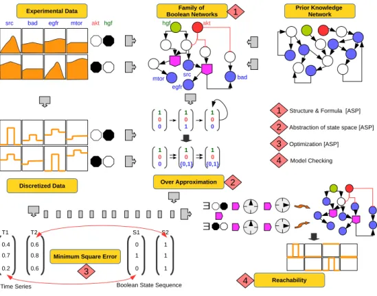
Fig 1. Generic workflow. Workflow illustrating the 4 step caspo-ts improved and adapted method used in this work. (1) A family of BNs is produced given protein perturbations (akt and hgf ) and a prior knowledge network, (2) BNs are filtered based on the verification of trajectories using the over-approximation criteria, (3) BNs are optimized based on the distance between the original time series and discretized data, (4) it is verified that there exist at least one path which satisfies the binarized
perturbation data. ASP stands for Answer Set Programming.
Experimental Data
src bad egfr mtor akt hgf
Prior Knowledge Network Family of Boolean Networks Discretized Data 0.4 0.7 0.2 0 1 0 1 1 1 0.6 0.8 0.6
Time Series Boolean State Sequence
T1 T2 S1 S2
Structure & Formula [ASP] Abstraction of state space [ASP] Optimization [ASP] Model Checking 1 2 3 4 2 3
Minimum Square Error
Over Approximation Reachability 4 ∃ ∃ 1 0 0 1 {0,1}0 1 {0,1}0 1 0 0 1 1 0 1 0 0 1 hgf akt mtor egfr bad src
Our results show that the Answer Set Programming (ASP) component of our method allows us to filter the explosion of possible dynamical states inherent to this type of problem, and thanks to that filtering, the model-checking step allows us to provide true positive BNs. Our results point to measurements in the time series DREAM 8 dataset that contradict the experimental setting and to perturbations that show contradictory dynamics. We observed that given the same PKN, the solving time was different for each cell line dataset, being the more complete for BT20, BT549, MCF7, while for the UACC812 cell line dataset it was impossible to find a true positive (TP) BN within a time-frame of 24 hours. This different structure of the solution space could point to incompatibilities of the dataset, which may give valuable insights for experimentalists. We also show that this method is capable of recovering time series measurements with a Root Mean Square Error (RMSE) of 0.31, the minimum achieved so far as compared to other participants of the DREAM 8 challenge. Based on a comparison with the canonical mTOR pathway, we show that the discovered context specific BNs had a True Positive Rate (TPR) of 82% on average. Computational time varies from one cell line to another depending on the number of perturbations and the order of the solution tree internally generated by the ASP solver. It took about 24 hours on average to generate TP BNs. We found 38% of the cell line specific interactions explaining the heterogeneity among
these four cancer cell lines, which can be observed in different cell specific networks, shown in S1 Fig, S2 Fig, S3 Fig and S4 Fig.
Results
Prior Knowledge Network
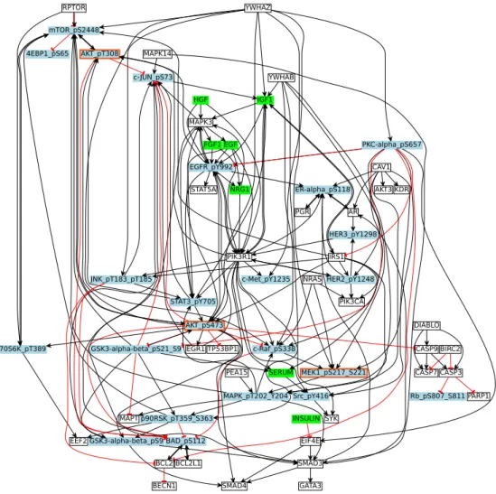
The structure of the signaling protein network was generated by mapping the experi-mentally measured phosphorylated proteins (DREAM 8 dataset) to their equivalents from literature-curated databases and connecting them together within a network. The reference network (Fig 2) was built using the ReactomeFIViz app (also called the Re-actomeFIPlugIn or Reactome FI Cytoscape app) [18], which accesses the interactions existing in the Reactome and other databases [18, 19].
In the context of our work, nodes are associated with stimuli, inhibitors and readouts, and are encoded by green, red and blue colors respectively. White nodes are unobserved nodes. The PKN shown in Fig 2 consists of 64 nodes (7 Stimuli, 3 Inhibitors, and 23 readouts) and 178 edges. Stimuli are used to bound the system and also serves as interaction points of the system. Inhibitors are those nodes which remain inactive or blocked over all time points of the experiment by small molecule inhibitors. Readouts are the measured nodes against perturbations (See Materials and Methods).
Fig 2. Breast Cancer Signaling Pathway. This figure shows the reconstructed signaling network from a combination of databases. An arrow shows the positive regulatory relationship between two proteins, while a T shaped arrow indicates inhibition. Green nodes are stimuli, blue nodes are readouts, white nodes are
unmeasured, and blue nodes with a red border represent inhibitors and readouts at the same time. White nodes are unobserved nodes. Stimuli, inhibitors and readouts have been defined in the text above. Please note that we have added the phosphorylation sites to the protein names in order to connect it to the experimental measurements.
mTOR_pS2448 AKT_pT308 AKT_pS473 p70S6K_pT389 4EBP1_pS65 MEK1_pS217_S221 MAPK_pT202_Y204 MAPK3 EGFR_pY992 FGF1 c-JUN_pS73 EGF STAT3_pY705 BAD_pS112 HER3_pY1298 PIK3R1 RPTOR HGF STAT5A NRG1 ER-alpha_pS118 IGF1 MAPT p90RSK_pT359_S363 GSK3-alpha-beta_pS9 EEF2 PKC-alpha_pS657 EIF4E c-Raf_pS338 GSK3-alpha-beta_pS21_S9 BCL2 IRS1 SMAD4 SMAD3 BECN1 AR PGR CAV1 KDR Src_pY416 HER2_pY1248 AKT3 GATA3 EGR1 PARP1 INSULIN YWHAZ c-Met_pY1235 JNK_pT183_pT185 BIRC2 CASP3 CASP7 Rb_pS807_S811 YWHAB NRAS PIK3CA CASP9 TP53BP1 BCL2L1 PEA15 SERUM SYK MAPK14 DIABLO
Data Processing
The dataset used here consists of four breast cancer cell lines - UACC812, BT20, BT549, and MCF7 [20, 21]. For the present study, we performed numerous data processing steps. The data from DREAM 8 contained values of measured proteins ranging over a variable range. We set the protein values between a common scale, i.e., 0 and 1, using a maximum-value-based normalization scheme (See Materials and Methods). Since the initial values for some time series were not available, controlled experimental readings have been used as the initial time point for each of these time series. There were a
few noisy and incomplete experiments. To resolve the issue of noisy data, one protein measurement was kept for each distinct time point of each noisy series. Experiments containing missing time points were removed to handle the time series incompleteness. There were some proteins which were inhibitors and readouts at the same time e.g., AKT and MEK1. We discovered that those proteins were showing abnormal behavior. For example, when a protein A is an inhibitor as well as a readout, then we observed an oscillatory behavior in the readout measurements of the protein A. We removed the experiments having such abnormal protein behavior. All data was refined and visualized using Matlab [22] and CellNOptR [23].
Cell Specific Boolean Networks
We used caspo-ts to model topology using a combination of existing knowledge (Fig 2) and the phosphoproteomic data of four breast cancer cell lines - BT20, BT549, MCF7, and UACC812. We inferred a family of cell specific BNs for each cancer cell line and they are shown in the Supplementary Figures (S1 Fig, S2 Fig, S3 Fig and S4 Fig).
The subset minimal solutions of different sizes for each cell line were obtained using the over-approximation criteria of caspo-ts within a few seconds (S1 Table). We put the restriction of 7 days to check the reachability of each solution using a model checker implemented as part of the caspo-ts tool. The number of verified solutions varies from one cell line to another, depending on a number of factors such as the number of perturbations, the order of answer sets in the solutions space, and the perturbation order. The total number of verified solutions within a constrained time are 231, 52, 188 and 150 for the BT549, MCF7, BT20 and UACC812 cell lines respectively. There were 191, 21, and 72 true positive BNs for BT549, MCF7, and BT20 cell lines respectively with an optimal fit to the data. The UACC812 cell line was more difficult to work with. We were unable to obtain true positive solutions by bounding it to the aforementioned time limit for verification. Hence, we kept the 20 BNs from UACC812 cell line confirming to the over-approximation criteria of caspo-ts method.
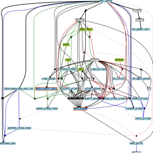
An aggregated network was built (Fig 3) by combining the BN families (with 191, 21, 72, and 20 BNs for BT549, MCF7, BT20, and UACC812 cell lines respectively) obtained for the four cell lines by keeping the hyper-edges (logic formulas) having a frequency higher than 0.3 within each BN family. This aggregated network contained 34 nodes and 74 boolean formulas involving 36 AND gates. As compared to the PKN (Fig 2), the inferred networks are strongly constrained to the context specificity. From Fig 3, we can see that all the cell lines share limited behaviors, however the similarity score varies if they are compared one by one with each other.
Fig 3. Boolean network of breast cancer cell lines. The aggregated graph for all cell lines. Blue, Red, Green and Pink colors have been used for each cell line BT20, BT549, MCF7 and UACC812 respectively. Inferred BNs consist of nodes connected by different edges (→ for activation and a for inhibition). Edges represent OR and AND gates. An AND gate is represented by a small black circle. An OR gate is represented by multiple edges pointing to a node. A different color scheme is used to represent different types of nodes. A green color is for stimuli, red is for inhibitors, blue is used to show readouts, and white is for unobserved nodes. Black edges are those edges which are common in cell lines, and the thickness of the edges represents the shared number of cell lines. BCL2L1 EGFR_pY992 . . . . . . . . . AKT_pT308 AKT_pS473 NRG1 STAT3_pY705 MAPK3 . BAD_pS112 . . . . ER-alpha_pS180 AR . GSK3-alpha-beta_pS21_S9 . . . . CASP9 p70S6K_pT389 GSK3-alpha-beta_pS9 . p90RSK_pT359_S363 c-Raf_pS338 CASP3 . JNK_pT803_pT805 . c-Met_pY1235 . EGF . . . PIK3R1 MEK1_pS217_S221 . MAPK_pT802_Y804 Rb_pS807_S811 . HER3_pY1298 4EBP1_pS65 . FGF1 . . . Src_pY416 IGF1 . . HER2_pY1248 . IRS1 mTOR_pS2448 HGF SERUM
In order to analyze the similarity among cell lines, we calculated the similarity score by applying Graph Similarity Algorithm (GSA) on family of BNs (with 191, 21, 72, and 20 BNs for BT549, MCF7, BT20, and UACC812 cell lines respectively) of breast cancer cell lines. This algorithm takes one gold standard network as an input and compares it to the family of BNs (See Materials and Methods). In our case, the gold standard network is the aggregation of one family of BNs. We keep the average of these similarity scores for each understudy breast cancer cell line shown in Table 1. Fig 3 agrees with
the results presented in Table 1 as we can see the clear discrepancies among the four cell lines. It can be seen that 23% of the boolean formulas are shared among BT549 and MCF7, and also between BT20 and UACC812. BT20 shares the least number of boolean formulas (15%) with BT549. This table revealed pronounced differences among different cell lines of breast cancer. Here, we also analyzed the diversity of boolean functions among the family of BNs within the same cell line. The similarity among boolean formulas from BT20 (0.73) and MCF7 (0.63) is higher than the BT549 (0.43) and UACC812 (0.46) cell lines.
Table 1. Similarity between four Breast Cancer Cell Lines. Family of BNs Cell Line
BT20 BT549 MCF7 UACC812 BT 20 0.73 0.15 0.17 0.23 BT 549 ∗∗ 0.43 0.23 0.20
M CF 7 ∗∗ ∗∗ 0.63 0.21
U ACC812 ∗∗ ∗∗ ∗∗ 0.46
The similarity analysis performed on each family of breast cancer cell lines i.e., BT20, BT549, MCF7 and UACC812. An aggregated network is generated for each cell line. Then the GSA is applied on each cell line. It computes the intersection between cell lines and generates the similarity score.
Heterogeneity among Cell Lines
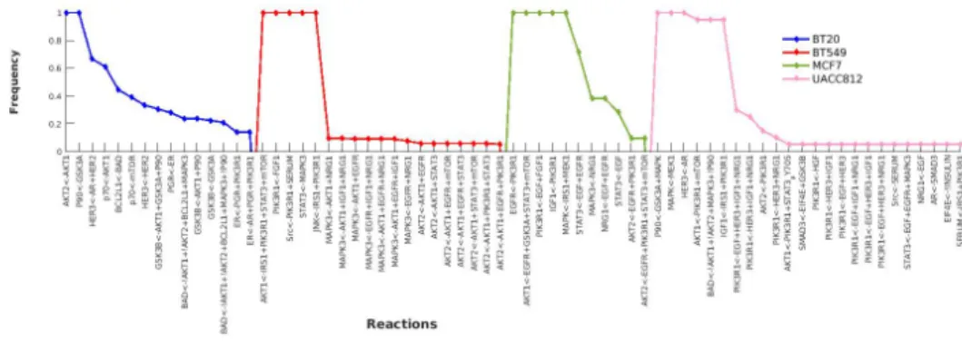
There are a total of 69 distinct boolean formulas shown in Fig 4 along with their respective frequencies. It is interesting to note that the B549 and UACC812 cell lines have more distinct models among their family of BNs with a variable frequency range. This shows that these cell lines have different mechanisms and strongly supports the effectiveness of our graph comparison algorithm.
Fig 4. Heterogeneous Behaviors. The discrepancies across all cell lines. Boolean formulas are represented on the X-axis and frequency of each boolean formula is shown on the Y-axis.
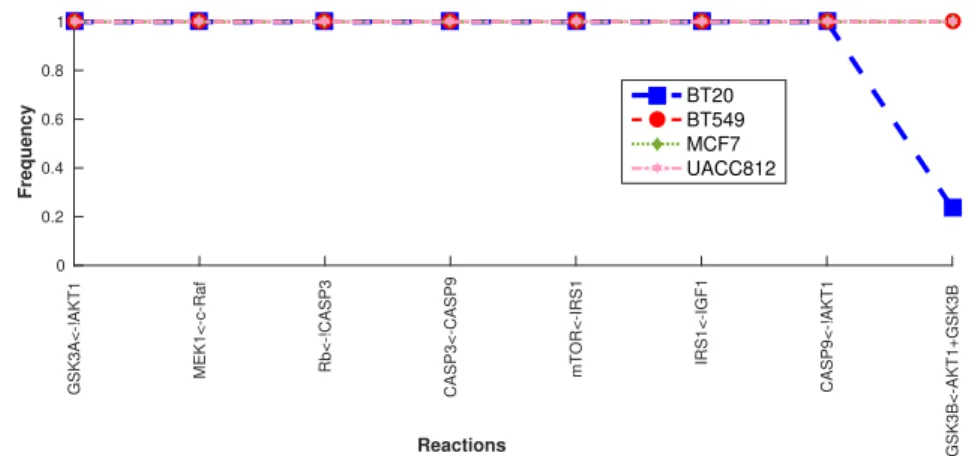
Fig 5 shows the common boolean formulas along with their frequency in all BNs. Interestingly, only 4% of the boolean formulas are shared and 99% of these shared formulas have the same frequency. In this figure, there is only one boolean formula which is frequent in 3 cell lines and has a lower frequency in BT20. Interestingly, all cell
lines share only 4% of boolean formulas and among them 99% have higher frequency in all the cell lines.
Fig 5. Common Behaviors across all four cell lines The commonalities among all cell lines. Boolean formulas are represented on the X-axis and frequency of each boolean formula is shown on the Y-axis.
GSK3A<-!AKT1 MEK1<-c-Raf Rb<-!CASP3 CASP3<-CASP9 mTOR<-IRS1 IRS1<-IGF1 CASP9<-!AKT1 GSK3B<-AKT1+GSK3B Reactions 0 0.2 0.4 0.6 0.8 1 Frequency BT20 BT549 MCF7 UACC812
Literature Knowledge about Behaviors discovered by caspo-ts
The union of each cell line is displayed in the Supplementary Figures (S1 Fig, S2 Fig, S3 Fig and S4 Fig). The caspo-ts method revealed that cell line specific reactions are clustered around the AKT, MAPK3, and PIK3R1 proteins. PI3K is an important factor for cancer development in HER2 amplified cancers (UACC812) as compared to non-HER2 amplified (BT20, BT549 and MCF7) cancer cell lines. We can see from the Supplementary Figures (S1 Fig, S2 Fig, S3 Fig and S4 Fig) that PIK3R1 exists in all cell lines but is rather more connected in the UACC812 cell line with the 10 incoming edges while in others with only 1 incoming edge. The PIK3R1 node in UACC812 (S4 Fig) has a centrality measure of 0.37 while in the other three cell lines the centrality measure is less than 0.11.
It has been established that P1K3R1 (the regulatory unit of PI3K) plays an important role in suppressing tumors [24, 25]. Recently, it has been found that PIK3R1 is mutated in 3% of breast cancer cell lines [26]. Nonetheless, it is worth studying the impact of the PIK3R1 regulatory unit in breast cancer.
Bcl-2 associated death promoter(BAD ) is regulated by AKT in triple negative breast cancer (TNBC) cell lines [27] and our method found the same in case of BT20 and BT549. In BT20 (S1 Fig), BAD is activated or inhibited through many signals. In BT549 (S2 Fig), BAD is regulated by AKT. In MCF7 (S3 Fig), BAD is activated by MAPK3 only. In UACC812 (S4 Fig), BAD is regulated by both AKT, MAPK3, and p90RSK. BAD is regulated differently in different breast cancer types emphasizing the importance of studying the context dependence functionality.
Validation w.r.t. Root Mean Square Error
The goal was not just to infer the best trained networks but also to verify that these networks are able to recover trajectories not existing in the experimental learning data. For this purpose, we are using experimental testing data to check the specificity of the
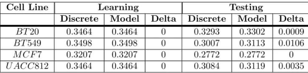
trajectories of the proposed networks. The data is provided by the DREAM8 challenge organizers (See Materials and Methods). We identify two types of RMSE: discrete and model. Discrete RMSE is imposed by the discretization of the method while model RMSE is the difference between the predictions of the BNs and the discretized data (See Materials and Methods). Table 2 shows the corresponding RMSE in case of learning and testing data. It can be seen that our cell specific Boolean models are able to produce the trajectories without any error in learning dataset for all cell lines. It is encouraging to see that predicted models are able to recover trajectories without any error in MCF7, with 0.0009 in BT20, with 0.0106 in BT549, and with 0.0035 in UACC812.
We also compared the RMSE score with the top two best performers of the DREAM8 challenge. We got the top position with a RMSE score of 0.31 as compared to their RMSE scores of 0.47 and 0.50. Our RMSE compares the trajectories predicted by Boolean models with the original trajectories existing in the testing data. In comparison to other DREAM 8 challenge methods based on Bayesian inference, Regression, and Granger Causality among others, we are not making new predictions but we are checking the recoverability of the testing trajectories by inferred BNs.
Table 2. Root Mean Square Error.
Cell Line Learning Testing
Discrete Model Delta Discrete Model Delta BT 20 0.3464 0.3464 0 0.3293 0.3302 0.0009 BT 549 0.3498 0.3498 0 0.3007 0.3113 0.0106 M CF 7 0.3207 0.3207 0 0.2772 0.2772 0 U ACC812 0.3464 0.3464 0 0.3084 0.3119 0.0035 Table 2 summarizes the statistical results. The cell line column shows the cell line under consideration. We have calculated discrete and model RMSE for the learning and testing datasets of each cell line. Delta shows the difference between discrete and model RMSE.
Validation w.r.t. Random Data Samples
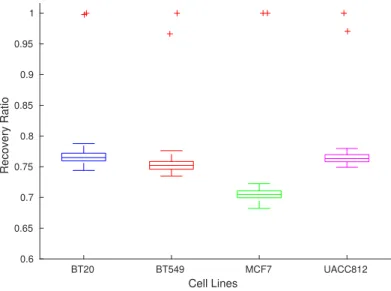
We generated 100 random data samples per cell line, then calculated the RMSE for the BNs of each cell line, and finally compared it with the learning and testing RMSE of these BNs. Fig 6 shows the performance of the method with respect to the learning, testing and random data. It can be observed that the method is unable to recover trajectories in the case of random data points without error as compared to the learning data, and to a maximum of 0.0106 of error in case of testing data. From Fig 6, It can be seen that learning and testing are clear outliers shown in red color in the case of all cell lines. It is worth noting that the caspo-ts method has failed to recover random data time series, hence proving the specificity of the learned networks with respect to DREAM 8 challenge data.
Fig 6. Performance Assessment w.r.t Learning, Testing and Random Dataset. Here, x axis shows the cell line and y axis shows the ratio of discrete and model RMSE for each respective cell line. Different cell lines are encoded by different color codes. Blue, Red, Green and Pink colors are used to denote BT20, BT549, MCF7 and UACC812 respectively.
BT20 BT549 MCF7 UACC812 Cell Lines 0.6 0.65 0.7 0.75 0.8 0.85 0.9 0.95 1 Recovery Ratio
Validation w.r.t. Canonical Pathway
To perform the validation, we compared the downstream nodes of the MTOR signaling cascade in the PKN with the downstream nodes of MTOR in cell specific BNs. True positive rate (TPR) and False positive rate (FPR) for each cell line was calculated using Equation (4) and (5) (See Materials and Methods). Fig 7 shows the Receiver Operating Characteristic (ROC) curve of each cell line according to their TPR and FPR. BT549 cell line models are the most accurate ones followed by MCF7 and BT20. We can observe the clear distinction between True Positive (TP) and False Positive (FP) BNs. In this case study, we were able to get TP BNs for the BT20, BT549 and MCF7 cell lines within approximately 24 hours. UACC812 cell line was the most difficult to deal with, making it difficult to get TP BNs within a reasonable computation time. We have obtained the a 0.77 AUROC score which is comparable to the 0.78 AUROC score of the top performing method of DREAM 8 challenge. A number of assumptions made during the modeling phase may have influenced our ranking. First, since our method can pinpoint the noisy, incomplete and erroneous experiment, it allows us to use only the reliable experimental settings. Second, our method constrains its solutions space to the proteins existing in the PKN, anything outside the background knowledge cannot be found. From figure 7, we can see that the method is quite promising for inferring TP BNs.
Fig 7. ROC curve. ROC curve across all cell lines. Here, the X-axis shows the FPR and the Y-axis denotes the TPR. Different cell lines are marked by different colors. The AUROC score is 0.77.
0 0.1 0.2 0.3 0.4 0.5 0.6 0.7 0.8 0.9 1
False Positive Rate
0 0.2 0.4 0.6 0.8 1
True Positive Rate
BT20 BT549 MCF7 UACC812
Discussion
In this paper, we build cell line specific signaling networks for a DREAM 8 time series dataset of 4 breast cancer cell lines (BT20, BT549, MCF7,and UACC812) using caspo-ts approach, which is a combination of Answer Set Programming and Model Checking methods. It allowed us to handle large-scale PKN (64 nodes and 178 edges) and real biological system. We were also interested in learning the dynamic properties of these networks explaining the time series data. Our results suggest that the behavior of cell line specific signaling network is highly variable even under same the perturbations, agreeing with the heterogeneity of breast cancer. We found that this method is capable of constructing cell line specific BNs, which is extremely valuable given heterogeneity of breast cancer due to many genetic modifications. Boolean models of each cell line are analyzed under different perturbation to identify commonalities as well as discrepancies. Moreover, these inferred models can be executed computationally to identify potential drug targets or to see the effect of unseen perturbations. The predictive power of the these models can be increased with improvements in protein interaction databases and comprehensive experimental data.
We have discovered 38% of the cell line dependent behaviors as compared to the 33% of the DREAM 8 challenge winner [28]. We have implemented an algorithm to analyze the variability among cell lines. We have also observed pairwise similarities among these cell lines. The similarity index varies from 15% (BT20 & BT549) to 23% (MCF7 & BT549, BT20 & MCF7). We have analyzed the similarity among family of BNs of the same cell line as well, which varies from 0.43 to 0.73. We have evaluated the accuracy of our method with RMSE and AUROC score 7. The maximum RMSE is 0.31 placing caspo-ts in first place in the DREAM 8 challenge. Various choices made during this study may have an impact on the final score. The caspo-ts method allowed us to remove noisy and faulty experiments, leaving us with the reliable experimental settings only. Here, we made the choice to use only reliable experiments instead of using all experimental settings. We did not observe all 45 proteins as we could not find connections in our PKN
for all the studied proteins, leaving us with approximately 23 proteins for each cell line. Nonetheless, the obtained results are quite promising, making caspo-ts a good candidate in the computational method tools. In fact, the caspo-ts method can be used to pinpoint the errors in the experimental data. We have discovered the experiments where protein AKT was inhibited but was having a dynamic behavior as a readout protein. Our work therefore provides a novel approach to show erroneous experiments which is very crucial and current approaches do not provide these insights, hence our method can be complement for the existing tools. The DREAM 8 dataset contained some noisy readings of experiments. Noisy experimental data reduces the efficiency of computational methods by posing the variability among constructed Boolean models. To overcome this, it is necessary to build automated methods to filter out the noisy experiments. This approach provides a step forward in building context dependent networks in the case of phosphoproteomic data. We are planning to investigate several aspects of this method, such as (i) the order of the solution space of over-approximated Boolean models; (ii) the computational time for checking reachability; (iii) design an efficient experimental design strategy and apply it prior to selecting the most informative experiment.
Perspective
The caspo-ts always gives answer sets in the same order because of the solver of ASP. It can be problematic in the case of large scale problems where we can not explore the whole solution space because of computational time constraint. We are currently working on sampling the solution space by splitting it to limit the number of considerable answer sets. We are also studying another feature to allow the diversity among subset minimal answer sets. It will be implemented by dynamically modifying the heuristic of the ASP solver at solving time. To reduce the false positive BNs rate, we are planning to use the multi-shot ASP technique. It solves the problem by customizing the logic problem at the solving step, hence generating a continuously modified logic program [29].
Materials and Methods
Data Acquisition
The DREAM portal provides unrestricted access to complex, pre-tested data to encourage the development of useful methods. In this study, we are focused on the DREAM 8 challenge, which was motivated by the fact that the same experimental conditions may lead to different signaling behaviors in different backgrounds, making it necessary to build a model which can perform unseen predictions (absent from the learning data). The main goal of the DREAM 8 challenge is to learn signaling networks efficiently and effectively to predict the dynamics of breast cancer [30].
Learning Data
Reverse Phase Protein Array (RPPA) quantitative proteomics technology was used for generating the dataset of this challenge. The measurements focus on short term changes on up to 45 proteins and their phosphorylation over 0 to 4 hours. The DREAM 8 dataset includes temporal changes in phosphorylated proteins at seven different time points (t1 = 0min, t2 = 5min, t3 = 15min, t4 = 30min, t5 = 60min, t6 = 120min, t7 = 240
min). Experimental data consists of of four cancer cell lines (BT20, BT549, MCF7 and UACC812) under different perturbations (≈8 stimuli and ≈3 inhibitors). In each cancer cell line, approximately 45 phosphorylated proteins are measured against different set of
perturbation over multiple time scales. In this study, we use the term perturbation to refer to the combination of stimuli and inhibitors, similarly to the other studies such as [20, 21, 30].
Testing Data
Test data is available for assessing the performance of networks learned from the experimental data. The DREAM 8 portal provides testing data for four cancer cell lines (BT20, BT549, MCF7 and UACC812) under different perturbations (8 stimuli and 1 inhibitor). They contain gold standard datasets of time series predictions of up to 45 proteins at seven different time points (t1= 0min, t2 = 5min, t3 = 15min, t4 =
30min, t5= 60min, t6= 120min, t7 = 240 min) [20, 21, 30]. This data is used to test the
performance of caspo-ts. Normalization
The protein measurements were ranging over variable ranges. Maximum value based normalization was used to set the measurements between a common scale, i.e., 0 and 1 in order to assign activation or inactivation values to variables or species of the BN. Equation 1 describes the formula used for the normalization:
zi,tp = x
p i,t
max(xpi,t) (1)
where i ∈ {1, . . . , n}, t ∈ {1, . . . , 7} , and p ∈ {1, . . . , 23}. xpi,t represents the value of protein p under perturbation i at time point t and max(xpi,t) denotes the highest value of protein p under all perturbations and time-points.
Prior Knowledge Network Derivation
PKNs are available in different databases such as Reactome, PID, and kegg among others [19, 31–42]. We can construct a PKN through different tools or softwares such as ReactomeFIViz [18] which is available as a Cytoscape [43] plugin. A PKN alone can not be used to build reliable dynamical models or to explain underlying biological behaviors [44], especially in the case of multiple perturbations data because of the need of specificity. In order to overcome this issue, methods have been proposed which take into account both literature based knowledge and experimental data to build logic models [3, 9–11, 44, 45]. In the context of our work, nodes in the PKN (Fig 2) are associated with stimuli, inhibitors and readouts and are encoded by different colors. Stimuli are represented by green, inhibitors by red and readouts by a blue color. Stimuli are those nodes which have no predecessors, are used to bound the system and also serve as entry points of the system. Inhibitors are those nodes which remain inactive or blocked over all time points of the experiment by small molecule inhibitors. Readouts are the nodes which are measured against given perturbations.
Network Reconstruction
For the reconstruction of BNs, we chose the caspo-ts method [14, 45]. This method was tailored to handle protein phosphoproteomic time series data. The input of the method consists of a prior knowledge network and normalized phosphoproteomic time series data under different perturbations to generate a family of BNs whose structure is compatible with the PKN and that can also reproduce the patterns observed in the experimental data.
The workflow of the reconstruction procedure is shown in Fig 1. It consists of four steps: 1) inference of a BN structure, 2) filtering of BNs according to time series data, 3) minimizing the distance between time series and discretized time series, 4) model checking of BNs to confirm that each condition given in phosphoproteomic data is satisfied. Experimental data consist of perturbations and readouts, where a perturbation is a combination of stimuli and inhibitors. In Fig 1, there are two perturbations involving akt (inhibitor) and hgf (stimulus): 1) akt =0, hgf =1 and 2) akt =1, hgf = 0. Black color means the value is 1 while white represents the value 0. Readouts are specified in a blue color and describe the time series under given perturbations.
Structure and Formula
A Boolean Network [46, 47] is defined as a pair b = (N ,F ), where
• N = {n1, ... , nk} is a finite set of nodes (or variables/proteins/genes)
• F = {f1, ... , fk} is a set of Boolean functions (regulatory functions) fi: Bk → B,
with B = {0, 1}, describing the evolution of variable ni.
A vector (or state) n(t) = (nt
1, ... , ntk) is the value of all nodes of N at time step t,
where nt
i represents the state of the node ni at time step t, and equals either 1 or 0.
There are up to 2k possible distinct states for each time step. If there is no update for
node ni then nt+1i = ni. If there is an update for node nithen the state of a node ni at
the next time step t + 1 is determined by nt+1i = fi(nti, ... ,ntk), with ni, ... ,nk are the
nodes directly influencing ni. Notice that usually only a subset influence the evolution
of node ni. These nodes are called the regulatory nodes of ni.
The state of each node can be updated in a synchronous (parallel) or asynchronous fashion. In the synchronous update schedule, the states of all nodes are updated synchronously, while in asynchronous update schedule, the state of one node can be updated at a time. The work presented in this article is independent of the update schedule routine, hence any number of nodes can be updated at a time.
The prior knowledge network is modeled as a labeled (or colored) directed graph with nodes V = {v1, v2, . . . , vm} associated to proteins and edges are labeled by −1
(v1a v2) or +1 (v1→ v2) depending on the interaction between proteins. Given a prior
knowledge network, a set of BNs B = {b1, b2, . . . , bq} are exhaustively enumerated where
each node mk of the bk ∈ B and k ∈ {1, . . . , q} has a formula compatible with the prior
knowledge network, meaning the regulatory nodes are the same. Please refer to [14] to know in detail about the enumeration process of BNs.
Abstraction of state space
After enumerating the set of BNs, experimental data is discretized in order to verify that trajectories can be reproduced through these BNs. The search space of BNs is generated by enumerating values for each node in a BN. Since the concrete search space is too large to handle, an abstract search space for the BN is generated to check the reachability of each node from another. Abstraction was achieved through over approximation to verify time series traces and was implemented in ASP. Please refer to [14,45] for implementation details. Over approximation was applied with the help of meta states which means that the previous value is retained through each sweep of the dynamic BN, resulting in the generation of false positive (FP) BNs. To resolve this issue, model checking is applied to rule out false positives.
Optimization
Root Mean Square Error (RMSE) refers to the distance between the actual time series zi,tp and the predicted time series yi,tp . We have adopted the formula in the ASP part of caspo-ts according to the DREAM 8 challenge.
RM SE = v u u t 1 23 ∗ 7 ∗ n 23 X p=1 7 X t=1 n X i=1 (zi,tp − ypi,t)2 (2)
If a BN can verify the time series traces of experimental data then it will have minimal MSE. But there may be some cases where it is not able to construct a BN which can reproduce all the time points of the trajectories. In that case, it will try to optimize the BN with the smallest distance possible.
Model Checking
To filter out the false positive BNs, exact model checking is applied. Computational tree logic (CTL) is used to check that there exists a path in the BN which can reproduce all trajectories under all experimental settings. CTL is a formal verification technique belonging to the branching temporal logic theory. Branching temporal refers to the fact that the future is not deterministic. The NuSMV model checker has been used to check the reachability of all experimental conditions [48].
Graph Similarity Algorithm (GSA)
This work introduces the study of a graph similarity measure in order to check the variability among the families of BNs generated by caspo-ts. The algorithm works by comparing the reactions existing in the gold standard network (A) with the family of BNs (B) and is based on the Jaccard similarity coefficient which measures the diversity of these models.
Jaccard Similarity Coefficient
The Jaccard index between A and Bican be defined as length of the intersection divided
by the union: J (A, Bi) = | A ∩ Bi| | A ∪ Bi| = | A ∩ Bi | | A | + | Bi| − | A ∩ Bi| (3) We apply the Jaccard Similarity Coefficient on Bi (the BN i where Bi ⊂ B) by taking
A as being the gold standard.
Evaluation
The performance of the caspo-ts method is evaluated using three criteria: 1) RMSE calcu-lation using a typical learning and testing data approach, 2) Random Data Comparison, 3) AUROC (Area Under the Operating Curve) score.
The Boolean networks are learned using the learning dataset only. The prediction accuracy is evaluated by comparing the RMSE of trajectories in the learning dataset and of those predicted by the learned networks. There are two types of RMSE - discrete and model. Discrete RMSE is associated with the method error. Since we use a BN discrete approach, our predicted traces will be in {0,1} and this introduces an error with respect to continuous measurements in [0,1]. Model RMSE refers to the learned BN model error, it will be larger than discrete RMSE when the BN model has some errors
in the predictions with respect to the discrete data. If the difference between these two is zero then inferred networks are able to recover the trajectories without any error.
In order to check if our method will produce random time series, we have generated random data samples for each perturbation and time point of the four cell lines. We have generated 100 random data files for each cell line. Finally, we applied the RMSE formula and compared the results with the testing and learning RMSE.
Next, the validity of these networks is verified by comparing them with the canonical MTOR signaling pathway using two parameters, i.e., true positive rate (TPR) and false positive rate (FPR). We calculated a set of nodes which should be modified under these unknown experimental settings and also exist in our PKN, called standard nodes. We evaluated how many of these nodes are modified in the learned networks, called modified nodes. TPR and FPR are defined by Equation (4) and Equation (5):
T P R = T P
T P + F N (4)
F P R = F P
F P + T N (5)
Here, TP is the number of nodes in the intersection between standard and inferred sets, FP is the number of nodes in the inferred set but not in the standard set, FN is the number of nodes in the standard set but not in the inferred set and TN is the number of nodes which are not in the standard set nor the inferred set. Finally, AUROC was drawn using TPR and FPR indicators.
Supporting Information
BCL2L1 . . BAD_pS112 Src_pY416 AKT_pS473 p70S6K_pT389 GSK3-alpha-beta_pS21_S9 . . AKT_pT308 . . CASP9 . GSK3-alpha-beta_pS9 p90RSK_pT359_S363 c-Raf_pS338 MAPK3 CASP3 c-Met_pY1235 c-JUN_pS73 IGF1 . IRS1 EGF EGFR_pY992 PIK3R1 MEK1_pS217_S221 . ER-alpha_pS118 PGR AR 4EBP1_pS65 . . HER2_pY1248 JNK_pT183_pT185 . HER3_pY1298 mTOR_pS2448 MAPK_pT202_Y204 Rb_pS807_S811S1 Fig. Union of BNs of BT20. Here, we show the union of BNs for the cell line BT20. This network is generated by combining 72 true positive BNs. It contains 31 nodes and 41 boolean functions with 12 AND gates. There are 2 stimuli, 2 inhibitors and 21 readouts. . AKT_pT308 BAD_pS112 Src_pY416 . . . . AKT_pS473 . . GSK3-alpha-beta_pS21_S9 . . . . . . . . . . . . CASP9 . MAPK3 GSK3-alpha-beta_pS9 p70S6K_pT389 CASP3 . . . c-Met_pY1235 Rb_pS807_S811 MEK1_pS217_S221 STAT3_pY705 FGF1 . . PIK3R1 4EBP1_pS65 . . c-Raf_pS338 . JNK_pT183_pT185 HER2_pY1248 NRG1 . . . . EGFR_pY992 IGF1 IRS1 mTOR_pS2448 MAPK_pT202_Y204 HGF SERUM
S2 Fig. Union of BNs of BT549. Here, we show the union of BNs for the cell line BT549. This networks is generated by combining 191 true positive BNs. It contains 28 nodes and 53 boolean functions with 35 AND gates. There are 5 stimuli, 2 inhibitors and 17 readouts. AKT_pS473 GSK3-alpha-beta_pS21_S9 . . CASP9 . p70S6K_pT389 GSK3-alpha-beta_pS9 CASP3 Rb_pS807_S811 . MAPK_pT202_Y204 BAD_pS112 EGF . . . STAT3_pY705 PIK3R1 NRG1 . . . . MEK1_pS217_S221 . AKT_pT308 MAPK3 FGF1 . EGFR_pY992 IGF1 . . ER-alpha_pS118 JNK_pT183_pT185 c-Raf_pS338 . IRS1 mTOR_pS2448
S3 Fig. Union of BNs of MCF7. Here, we show the union of BNs for the cell line MCF7. This network is generated by combining 21 true positive BNs. It contains 24 nodes and 37 boolean functions with 19 AND gates. There are 4 stimuli, 2 inhibitors and 15 readouts.
. AKT_pT308 . Src_pY416 . . . p90RSK_pT359_S363 . GSK3-alpha-beta_pS9 . . ER-alpha_pS118 AR . . SERUM AKT_pS473 GSK3-alpha-beta_pS21_S9 . . CASP9 . BAD_pS112 c-Raf_pS338 MAPK3 CASP3 p70S6K_pT389 SMAD3 HER3_pY1298 Rb_pS807_S811 HGF PIK3R1 EGFR_pY992 . . . . HER2_pY1248 . STAT3_pY705 . EGF NRG1 . . . . . . . . . MEK1_pS217_S221 MAPK_pT202_Y204 . 4EBP1_pS65 IGF1 IRS1 mTOR_pS2448 INSULIN EIF4E
S4 Fig. Union of BNs of UACC812. Here, we show the union of BNs for the cell line UACC812. This network is generated by combining 20 BNs. It contains 33 nodes and 54 boolean functions with 29 AND gates. There are 6 stimuli, 2 inhibitors and 18 readouts.
Cell Line Number of Solutions True Positives False Positives Time
Computation Validation
BT 20 188 72 116 210 seconds 7 days
BT 549 231 191 40 93 seconds 7 days
M CF 7 52 21 21 36 seconds 7 days
U ACC812 150 0 150 197 seconds 7 days
S1 Table. Computation Summary. Here, we show the number of solutions, true positive and false positive BNs, and their computation (Solving) and validation (Model Checking) time for each cell line. We generated 32 true positive solutions for UACC812 cell line by allowing the model checker to run without bounding it to the aforementioned time limit.
References
1. Watterson S, Marshall S, Ghazal P. Logic models of pathway biology. Drug discovery today. 2008;13(9):447–456.
2. Samaga R, Klamt S. Modeling approaches for qualitative and semi-quantitative analysis of cellular signaling networks. Cell communication and signaling. 2013;11(1):43.
3. MacNamara A, Terfve C, Henriques D, Bernab´e BP, Saez-Rodriguez J. State–time spectrum of signal transduction logic models. Physical biology. 2012;9(4):045003. 4. Kauffman SA. The origins of order: Self-organization and selection in evolution.
Oxford University Press, USA; 1993.
5. Thomas R. Laws for the dynamics of regulatory networks. International Journal of Developmental Biology. 2002;42(3):479–485.
6. Albert R, Othmer HG. The topology of the regulatory interactions predicts the expression pattern of the segment polarity genes in Drosophila melanogaster. Journal of theoretical biology. 2003;223(1):1–18.
7. Akman OE, Watterson S, Parton A, Binns N, Millar AJ, Ghazal P. Digital clocks: simple Boolean models can quantitatively describe circadian systems. Journal of The Royal Society Interface. 2012; p. rsif20120080.
8. Wynn ML, Consul N, Merajver SD, Schnell S. Logic-based models in systems biology: a predictive and parameter-free network analysis method. Integrative biology. 2012;4(11):1323–1337.
9. Saez-Rodriguez J, Alexopoulos LG, Epperlein J, Samaga R, Lauffenburger DA, Klamt S, et al. Discrete logic modelling as a means to link protein signalling networks with functional analysis of mammalian signal transduction. Molecular systems biology. 2009;5(1).
10. Guziolowski C, Videla S, Eduati F, Thiele S, Cokelaer T, Siegel A, et al. Exhaus-tively characterizing feasible logic models of a signaling network using answer set programming. Bioinformatics. 2013;29(18):2320–2326.
11. Videla S, Guziolowski C, Eduati F, Thiele S, Grabe N, Saez-Rodriguez J, et al. Revisiting the training of logic models of protein signaling networks with ASP. In: Computational Methods in Systems Biology. Springer; 2012. p. 342–361.
12. Mitsos A, Melas IN, Siminelakis P, Chairakaki AD, Saez-Rodriguez J, Alex-opoulos LG. Identifying drug effects via pathway alterations using an integer linear programming optimization formulation on phosphoproteomic data. PLoS computational biology. 2009;5(12):e1000591.
13. Sharan R, Karp RM. Reconstructing Boolean models of signaling. Journal of Computational Biology. 2013;20(3):249–257.
14. Ostrowski M, Paulev´e L, Schaub T, Siegel A, Guziolowski C. Boolean network identification from perturbation time series data combining dynamics abstraction and logic programming. Biosystems. 2016;149:139–153.
15. Dorier J, Crespo I, Niknejad A, Liechti R, Ebeling M, Xenarios I. Boolean regulatory network reconstruction using literature based knowledge with a genetic algorithm optimization method. BMC bioinformatics. 2016;17(1):410.
16. Almudevar A, McCall MN, McMurray H, Land H. Fitting Boolean networks from steady state perturbation data. Statistical applications in genetics and molecular biology. 2011;10(1):47.
17. Zhu P, Aliabadi HM, Uluda˘g H, Han J. Identification of Potential Drug Targets in Cancer Signaling Pathways using Stochastic Logical Models. Scientific reports. 2016;6.
18. Wu G, Dawson E, Duong A, Haw R, Stein L. ReactomeFIViz: a Cytoscape app for pathway and network-based data analysis. F1000Research. 2014;3.
19. Wu G, Dawson E, Duong A, Haw R, Stein L. ReactomeFIViz: a Cytoscape app for pathway and network-based data analysis. F1000Research. 2014;3.
20. Hill SM, Nesser NK, Johnson-Camacho K, Jeffress M, Johnson A, Boniface C, et al. Context specificity in causal signaling networks revealed by phosphoprotein profiling. Cell systems. 2017;4(1):73–83.
21. Hill SM, Heiser LM, Cokelaer T, Unger M, Nesser NK, Carlin DE, et al. Inferring causal molecular networks: empirical assessment through a community-based effort. Nature methods. 2016;13(4):310–318.
22. MathWorks I. MATLAB and Statistics Toolbox Release; 2012.
23. Terfve C, Cokelaer T, MacNamara A, Saez-Rodriguez J. Training of boolean logic models of signalling networks using prior knowledge networks and perturbation data with CellNOptR. 2013;.
24. Shekar SC, Wu H, Fu Z, Yip SC, Cahill SM, Girvin ME, et al. Mechanism of constitutive phosphoinositide 3-kinase activation by oncogenic mutants of the p85 regulatory subunit. Journal of Biological Chemistry. 2005;280(30):27850–27855. 25. Taniguchi CM, Winnay J, Kondo T, Bronson RT, Guimaraes AR, Alem´an JO, et al.
The phosphoinositide 3-kinase regulatory subunit p85α can exert tumor suppressor properties through negative regulation of growth factor signaling. Cancer research. 2010;70(13):5305–5315.
26. Network CGA, et al.. Comprehensive molecular portraits of human breast tumours. Nature 490, 61e70; 2012.
27. Nassirpour R, Mehta P, M Baxi S, Yin MJ. miR-221 Promotes Tumorigenesis in Human Triple Negative Breast Cancer Cells. 2013;8:e62170.
28. Carlin DE. Computational evaluation and derivation of biological networks in cancer and stem cells. University of California, Santa Cruz; 2014.
29. Kaminski R, Schaub T, Wanko P. A tutorial on hybrid answer set solving with clingo. In: Reasoning Web International Summer School. Springer; 2017. p. 167–203.
30. Heiser L. HPN-DREAM breast cancer network inference challenge; 2016. https:// www.synapse.org/#!Synapse:syn1720047/wiki/55342. Available from: https: //www.synapse.org/#!Synapse:syn1720047/wiki/55342.
31. Duan G, Walther D. The roles of post-translational modifications in the context of protein interaction networks. PLoS Comput Biol. 2015;11(2):e1004049. 32. Kanehisa M, Goto S. KEGG: kyoto encyclopedia of genes and genomes. Nucleic
acids research. 2000;28(1):27–30.
33. Consortium GO, et al. The Gene Ontology (GO) database and informatics resource. Nucleic acids research. 2004;32(suppl 1):D258–D261.
34. Kelder T, van Iersel MP, Hanspers K, Kutmon M, Conklin BR, Evelo CT, et al. WikiPathways: building research communities on biological pathways. Nucleic Acids Research. 2012;40(D1):D1301. doi:10.1093/nar/gkr1074.
35. Nishimura D. BioCarta. Biotech Software & Internet Report: The Computer Software Journal for Scient. 2001;2(3):117–120.
36. Stark C, Breitkreutz BJ, Reguly T, Boucher L, Breitkreutz A, Tyers M. Bi-oGRID: a general repository for interaction datasets. Nucleic acids research. 2006;34(suppl 1):D535–D539.
37. Szklarczyk D, Morris JH, Cook H, Kuhn M, Wyder S, Simonovic M, et al. The STRING database in 2017: quality-controlled protein–protein association networks, made broadly accessible. Nucleic acids research. 2017;45(D1):D362–D368. 38. Xenarios I, Rice DW, Salwinski L, Baron MK, Marcotte EM, Eisenberg D. DIP:
the database of interacting proteins. Nucleic acids research. 2000;28(1):289–291. 39. Peri S, Navarro JD, Kristiansen TZ, Amanchy R, Surendranath V, Muthusamy B,
et al. Human protein reference database as a discovery resource for proteomics. Nucleic acids research. 2004;32(suppl 1):D497–D501.
40. Hermjakob H, Montecchi-Palazzi L, Lewington C, Mudali S, Kerrien S, Orchard S, et al. IntAct: an open source molecular interaction database. Nucleic acids research. 2004;32(suppl 1):D452–D455.
41. Zanzoni A, Montecchi-Palazzi L, Quondam M, Ausiello G, Helmer-Citterich M, Ce-sareni G. MINT: a Molecular INTeraction database. FEBS letters. 2002;513(1):135– 140.
42. Razick S, Magklaras G, Donaldson IM. iRefIndex: a consolidated protein interac-tion database with provenance. BMC bioinformatics. 2008;9(1):405.
43. Shannon P, Markiel A, Ozier O, Baliga NS, Wang JT, Ramage D, et al. Cytoscape: a software environment for integrated models of biomolecular interaction networks. Genome research. 2003;13(11):2498–2504.
44. Rodriguez A, Crespo I, Androsova G, del Sol A. Discrete Logic Modelling Optimization to Contextualize Prior Knowledge Networks Using PRUNET. PloS one. 2015;10(6):e0127216.
45. Ostrowski M, Paulev´e L, Schaub T, Siegel A, Guziolowski C. Boolean Network Identification from Multiplex Time Series Data. In: Computational Methods in Systems Biology. vol. 9308. Springer; 2015. p. 170–181.
46. Kauffman SA. Metabolic stability and epigenesis in randomly constructed genetic nets. Journal of theoretical biology. 1969;22(3):437–467.
47. Inoue K. Logic programming for Boolean networks. In: IJCAI Proceedings-International Joint Conference on Artificial Intelligence. vol. 22. Citeseer; 2011. p. 924.
48. Cimatti A, Clarke E, Giunchiglia E, Giunchiglia F, Pistore M, Roveri M, et al. Nusmv 2: An opensource tool for symbolic model checking. In: International Conference on Computer Aided Verification. Springer; 2002. p. 359–364.