HAL Id: hal-01347804
https://hal.archives-ouvertes.fr/hal-01347804
Submitted on 7 Sep 2016HAL is a multi-disciplinary open access
archive for the deposit and dissemination of sci-entific research documents, whether they are pub-lished or not. The documents may come from teaching and research institutions in France or abroad, or from public or private research centers.
L’archive ouverte pluridisciplinaire HAL, est destinée au dépôt et à la diffusion de documents scientifiques de niveau recherche, publiés ou non, émanant des établissements d’enseignement et de recherche français ou étrangers, des laboratoires publics ou privés.
Nourhene Ettouzi, Philippe Leray, Montassar Ben Messaoud
To cite this version:
Nourhene Ettouzi, Philippe Leray, Montassar Ben Messaoud. An exact approach to learning proba-bilistic relational model. 8th International Conference on Probaproba-bilistic Graphical Models (PGM 2016), 2016, Lugano, Switzerland. pp.171-182. �hal-01347804�
An Exact Approach to Learning Probabilistic Relational Model
Nourhene Ettouzi [email protected]
LARODEC, ISG Sousse, Tunisia
Philippe Leray [email protected]
LINA, DUke research group University of Nantes, France
Montassar Ben Messaoud [email protected]
LARODEC, ISG Tunis, Tunisia
Abstract
Probabilistic Graphical Models (PGMs) offer a popular framework including a variety of statistical formalisms, such as Bayesian networks (BNs). These latter are able to depict real-world situations with high degree of uncertainty. Due to their power and flexibility, several extensions were pro-posed, ensuring thereby the suitability of their use. Probabilistic Relational Models (PRMs) extend BNs to work with relational databases rather than propositional data. Their construction represents an active area since it remains the most complicated issue. Only few works have been proposed in this direction, and most of them don’t guarantee an optimal identification of their dependency structure. In this paper we intend to propose an approach that ensures returning an optimal PRM structure. It is inspired from a BN method whose performance was already proven.
Keywords: Exact structure learning, Probabilistic Relational Models, A* search.
1. Introduction
Bayesian networks (BNs) combine two powerful theories: probability and graph theories. They build a graphical representation of real-world problems. Score-based methods are very suitable for building models from data, that correspond most closely to reality (Cooper and Herskovits, 1992). Search approaches are divided into two main families: approximate methods with a convergence to a local optimum, and exact methods which are sometimes costly in time and space but guarantee finding globally optimal models. (Yuan et al., 2011) presents a new approach formulating the BN structure learning process as a search graph problem. The algorithm focuses on searching on the most promising parts of the graph with the guidance of a consistent heuristic. Their strategy is shown to effectively find an optimal BN.
Married with relational representation, BNs are extended to Probabilistic Relational Models (PRMs) (Koller and Pfeffer, 1998). PRMs offer a rich language for representing relational data whose large amounts become unmanageable. Only few works have been proposed to learn its prob-abilistic structure. (Getoor et al., 2001) have proposed a relational extension of an approximate score-based approach. A constraint-based approach extended on the relational context have been developped in (Maier et al., 2010) while (Ben Ishak, 2015) has proposed a relational hybrid ap-proach. To the best of our knowledge, no previous works have already investigated the relational exact structure learning. It is from this perspective that the present paper will attempt to propose a new exact approach to learn PRMs structure, inspired from (Yuan et al., 2011).
The remainder of this paper is organized as follows: section 2 provides a brief recall on BNs emphasizing the exact approach presented by (Yuan et al., 2011) and PRMs . Section 3 describes our new approach for learning PRMs structure. Section 4 finally presents an example trace of our approach.
2. Background
We propose in this section to give a brief recall of definitions and structure learning approaches of BNs and PRMs.
2.1 Bayesian Networks
BNs are one of the widely-used Probabilistic Graphical Models (PGMs) which represent an effective tool for solving problems in artificial intelligence, especially for representing knowledge under uncertainty.
2.1.1 DEFINITION
A BN is encoded by a Directed Acyclic Graph (DAG) whose structure is defined by two sets: the set of nodes representing discrete random variables, and the set of edges representing dependencies between adjacent variables. In addition to the structure considered as a qualitative component, a quantitative component is specified to describe the Conditional Probability Distributions (CPDs) of each variable given its parents in the graph.
2.1.2 EXACTSTRUCTURELEARNING
BN structure learning takes data D as input and produces the structure network that best fits D. There are three main families of structure learning task namely score-based, constraint-based and hybrid approach. For the score-based family, the idea is to evaluate the compliance of the structure to the data using a scoring function and find the best structure using a search strategy.
• Scoring Function: The degree of the fitness of the network is measured using a scoring func-tion. Several scoring functions can be used, for instance, Bayesian Dirichlet (BD) Score and its variants, Minimum Description Length or Akaike Information Criterion, etc. The most important property of scoring functions is their decomposability. A scoring function is de-composable if the score of the structure, Score(BN(V)), can be expressed as the sum of local scores at each node.
Score(BN (V)) = X
X∈V
Score(X | P aX) (1)
Each one, Score(X | P aX), is a function of one node and its parents. On the other hand
these scoring functions have one slight difference. Some scores need to be maximized and others need to be minimized in order to find optimal structure. By simply changing the sign of the scores, the translation between maximization and minimisation is straightforward. We will consider in the later the minimization of the scoring function.
• Search strategy: Using an exhaustive approach to search BN structure is impossible in prac-tice. Given n variables, there are O(n2n(n−1)) DAGs (Chickering, 1996). It is thus an NP-hard task. Since that several approaches were proposed. These approaches are divided on two
main classes. First exact approaches are based on optimal search strategies. In the opposite, approximate approachesare based on local search strategies such as greedy hill climbing. The search algorithm identifies candidate structures and scores them. The structures having best scores are then used to identify new candidates. A critical drawback in local search methods is that the quality of their solutions is still unknown. This had let researchers to cast exact structure learning algorithms to provably optimize the scoring function.
Several exact algorithms have been developed for learning optimal BNs such as Mathematical Programming(Cussens, 2012), Branch and Bound (BB) (de Campos and Ji, 2011), Dynamic Pro-gramming (DP)(Chen et al., 2013) and Heuristic Search (Yuan et al., 2011). The DP derives from the observation that BNs are DAGs and DAGs have a topological ordering. Thus, identifying the optimal BN structure attempts to specify the ordering of variables. This optimal BN is considered as a set of optimal subnetworks. Each one contains a leaf variable and its optimal parents. The algorithm uses the equations 2 and 3 to find recursively leaves of subnetworks:
Score(V) = min X∈V{Score(V\{X}) + BestScore(X | V\{X})} (2) where BestScore(X | V\{X}) = min P aX⊂V\{X} Score(X | P aX) (3)
Given a set of variables V, BN∗(V) represents the optimal BN defined over V and Score(V)= Score(BN∗(V)). At each iteration X is selected as the leaf, an optimal subnetwork is constructed by choosing an optimal parent set P aX from the remaining variables V\{X} and BestScore(X,
V\{X}) gives the best score of the latter subnetwork. The DP algorithm uses an order graph as a way to explore the space over the possible V by optimizing equation 2 and a parent graph for each variable to search its optimal parents by optimizing equation 3. DP evaluates all the possible order-ings and all intermediate results are stored in memory. As the search space increases, computing and storing graphs become impossible. That is the major drawback of that approach.
(Yuan and Malone, 2013) address this critical issue and propose the use of A* search (Hart et al., 1968) to learn optimal BNs structure. This approach aims also to search the topological order of variables, by defining the shortest path between the top-most and the bottom-most node. Thus the optimal BN structure learning problem is formulated as a shortest path finding process. To remedy the flaw of high time and space complexity, heuristics are used. Best First Heuristic search (BFHS) (Pearl, 1984) is an example of such an heuristic to find the shortest path and then deduce an optimal BN.
As in DP approach, this search uses an order graph as a solution space and a parent graph for each variable to identify its optimal parent sets and their corresponding best scores. It restricts the search to the most promising parts of the solution space. BFHS expands nodes in the order of their quality defined by an evaluation function f that measures the qualities of nodes. BFHS has several variants and each one evaluates the node’s quality in a different manner. (Yuan and Malone, 2013) uses A* search and defines f as the sum of g- and h-values. g-value represents the exact cost so far from the start node and h-value represents an estimated distance to the goal.
The algorithm uses a priority queue, called open list to organize the search. It is initialized with the start state. At each iteration, the node in the open list having the smallest cost is selected to expand its successor nodes. Then it is placed in a closed list. If a duplicate is detected in the open list (resp. closed list), the node having the lower g-cost is kept, the other node will be discarded.
Once the goal node is selected for expansion, the complete path is found where each arc corresponds to the optimal parent set for each variable, defining the optimal BN.
For each node, the g-value is the sum of edge costs on the best path from the start node to that node. Each edge cost is computed when a successor is generated and its value is retrieved from a corresponding node in the parent graph. Only some edge costs need to be computed as the A* search explores just a small part of the order graph.
The h-cost is computed using heuristic function. It represents basically the lower bound of the search, and must be admissible (i.e. never over estimates the distance) and consistent (i.e. never decreases in any path). Once h is consistent, automatically it is admissible, because consistency implies admissibility. And once h is admissible, A* search is optimal and the progressed path is the shortest one. Let U be a node in the order graph that contains a set of variables. The heuristic function shown in equation 4 was proposed and its consistency and admissibility were proven in (Yuan et al., 2011). h(U ) enables variables not yet present in the ordering to choose their optimal parents from V.
h(U ) = X
X∈V\U
BestScore(X | V\{X}) (4)
Several empirical studies were conducted in (Yuan and Malone, 2013) and results proved the effectiveness of A* search. In addition, the A* search outperforms BB approach by preserving the acyclicity constraint whereas BB needs to detect and break cycles. It outperforms also the DP approach by restricting the search to the most promising part of the graph. That partial graph search is guaranteed to be optimal thanks to the consistency and the admissibility of the heuristic function. 2.2 Probabilistic Relational Models
Despite their success, BNs are often inadequate for representing complex domains such as relational databases. In fact, BNs are developed for flat data. However data management practices have taken further aspects. They present a large number of dimensions, with different types of entities. BNs are extended to work in a relational context giving birth to Probabilistic Relational Models (Getoor and Taskar, 2007; Koller and Pfeffer, 1998; Pfeffer, 2000).
2.2.1 DEFINITION
Before presenting the formal definition of PRMs, some definitions related to the relational context must be mentioned. Given a relational schema R, we denote X the set of all the classes and A(X) the set of all descriptive attributes of a class X ∈ X . To manage references between objects, we use reference slots.
Definition 1 Reference Slot. For a class X ∈ X , X.ρ denotes its reference slot (targeting one classY ) where X is a domain type and Y is a range type, Y ∈ X . A reversed slot ρ−1 can be defined for each reference slotρ.
Definition 2 Slot chain. A slot chain K is a sequence of reference slots (reversed or not) ρ1,...,ρk,
where∀i, Range[ρi] = Dom[ρi+1].
Definition 3 Aggregate function. An aggregate function γ takes as input values of a multi-set and returns a summary of it. AVG, MAX and MIN are examples of aggregate functions.
Movie Transaction User rdate genre rating gender mo us Movie.genre Transaction.rating Low High Drama, M 0.9 0.1 Drama, F 0.3 0.7 Horror,M 0.8 0.2 Comedy, M 0.5 0.5 Comedy, F 0.6 0.4 Use r.ge nd er User.gender M F 0.5 0.5 Movie.genre Drama Horror Comedy
0.3 0.3 0.4
Figure 1: An example of a PRM. R is the relational schema described in example 1. The depen-dency structure S is depicted by the plain arrows between the attributes.
Definition 4 Probabilistic relational model. (Getoor and Taskar, 2007) define formally a PRM associated to a relational schemaR by :
• A dependency structure S: Each attribute A ∈ A(X) of a class X ∈ X has a set of parents P a(X.A) that describes probabilistic dependencies. If that parent is a simple attribute in the same class, it has the form ofX.B, B ∈ A(X). It can also have the more general form of γ(X.K.B) when referencing an attribute B related to the starting class X with a slot chain K andγ is an aggregate function.
• A set of CPDs ΘSrepresentingP (X.A | P a(X.A)).
We note that increasing the slot chain length may lead to the generation of a more complex models. That is why it is usual to limit it to a maximum slot chain length (Kmax).
Example 1 Let us consider an example of a relational schema R for a simple movie domain. There are three classes: Movie, Transaction and User. The class Movie has Movie.genre and Movie.rdate as descriptive attributes (rdate denotes movie’s release date). The class Transaction refers both Movie and User classes with respectively two reference slots Transaction.mo and Transaction.us, where range[T ransaction.mo] is Movie and range[T ransaction.us] is User.
An example of a PRM associated to the movie domain is depicted in Figure 1. An example of probabilistic dependency with a slot chain length equal to 1 is Transaction.User.gender→ Trans-action.rating, where Transaction.User.gender is the parent and Transaction.rating is the child.
Each time we vary the slot chain length, other probabilistic dependencies appear. Setting, for
in-stance, the slot chain length to 3, a probabilistic dependency betweenγ(transaction.Movie.mo−1.User.gender) and Transaction.rating may appear.
2.2.2 PRM STRUCTURE LEARNING
PRMs construction states finding its structure S and providing subsequently its parameters ΘS.
Works in this area are very rare, and (Getoor et al., 2001) is the main score-based approach proposed to learn PRMs structure. Adapting the (decomposable) BD score in the relational context, they proposed a local search method where an usual Greedy Hill Climbing search is embedded in a loop where the length of the possible slot chains increases at each step. However, with such approximate approach, there is no guarantee that the returned solution is optimal.
3. Relational BFHS: A New Approach to Learning Probabilistic Relational Models
The BFHS search described in section 2.1.2 is able to learn effectively BN structures using a heuris-tic function to restrict the search space to the most promising parts of the solution space. Our main idea, in this paper, is to adapt this process to the relational context. That is possible thanks to the decomposabilityproperty of the PRM scoring function. Our proposal consists of an exact approach to learn the structure of a PRM from a complete relational dataset. We call it Relational Best First Heuristic Search, Relational BFHS for short. Given the relational schema that describes the domain and a fully specified instance of that schema, our main contributions consists in the definition of the order graph, the parent graph, the cost so far function and the heuristic function, adapted in the relational context. A* search can be then applied exactly as in the BN learning process to find an optimal PRM structure.
3.1 Relational Order Graph
Let us denote X .A = {Xi.A} where i ∈ [1..n], n is the number of classes in R, Xi ∈ X and A ∈
A(Xi) the set of all attributes of the classes in R.
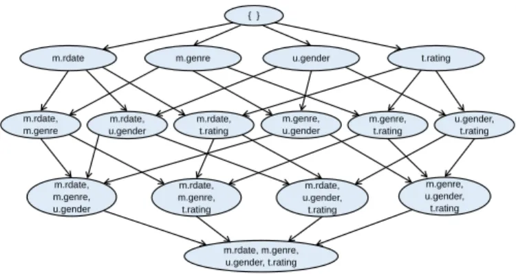
Definition 5 A relational order graph related to a relational schema R is a lattice over 2X .A, powerset ofX .A. A relational order graph holds then the elements of 2X .Aordered with respect to inclusion. Each node U corresponds to a subset ofX .A. The top-most node in level 0 containing the empty set is the start node. The bottom-most one containing the setX .A is the goal node. Each edge corresponds to adding a new attributeY.B in the model, and has a cost equal to BestScore(Y.B|..). This best score will be given by the parent graph ofY.B defined in the next section.
Example 2 Figure 2 displays the relational order graph related to the relational schema R depicted in example 1. For short, we use t, m and u to denote respectively Transaction, Movie and User. Each node stores an element of the powerset of the setX .A = {Movie.genre, Movie.rdate, User.gender, Transaction.rating}.
The relational order graph represents our solution space. With our relational models, one at-tribute A can be a potential parent of itself, via several slot chains K (for instance, the color of the eyes of one person depends of the color of the eyes of his mother and the one of his father). So, the dependency structure S describing the parenthood relationships is an extended DAG where we accept loops, i.e edges from one attribute to itself. A directed path in our relational order graph, from the start node to any node U yields an ordering on the attributes in that path with new attributes appearing layer by layer (and this attribute itself). Finding the shortest path from the start node to the goal node corresponds to identifying the optimal dependency structure S of our PRM.
{ } m.genre t.rating m.rdate u.gender m.rdate, m.genre m.rdate, u.gender m.rdate, t.rating m.genre, u.gender m.genre, t.rating u.gender, t.rating m.rdate, m.genre, u.gender m.rdate, m.genre, t.rating m.rdate, u.gender, t.rating m.genre, u.gender, t.rating m.rdate, m.genre, u.gender, t.rating
Figure 2: Our relational order graph related to R. 3.2 Relational Parent Graph
One parent graph is defined for each attribute Xi.A. Let us denote CP a(Xi.A) = {CP aj} the
candidate parents set of Xi.A. As stated in definition 4, the general form of each parent is γ(X.K.B),
referencing an attribute B related to the starting class X with a slot chain K and γ a potential aggregate function.
Definition 6 A relational parent graph of an attribute Xi.A is a lattice over2CP a(Xi.A), powerset of
the candidate parents of this attributeCP a(Xi.A), for a given maximal length of slot chain Kmax.
Each node V in the relational parent graph of an attribute Xi.A corresponds to a subset of
CPa(Xi.A). This parent graph will help to store the local score of this attribute given this particular
candidate parent set and identify the best possible parents for this attribute.
Example 3 Figure 3 shows the relational parent graph of Movie.genre using slot chains of maxi-mum lengthKmax= 2 and one only aggregate function. We use us−1andmo−1to denote
respec-tively the reference slot of User and Movie. The first layer of that graph contains the three can-didate parents for Movie.rating, CPa(Movie.rating) ={Movie.rdate, γ(Movie.mo−1.User.gender),
γ(Movie.mo−1.rating)}. The first node in level 2 of the relational parent graph corresponds to the set composed of Movie.rdate andγ(Movie.mo−1.User.gender) as candidate parents for Movie.genre. Our relational parent graph looks like the BN parent graph except that in the latter, the candidate parents of one attribute are the other attributes. Whereas our relational parent graph, the set of candidate parents is generated from the relational schema and a maximal slot chain length and one attribute can appear in its own relational parent graph.
Example 4 With K = 4, we can have a probabilistic dependency from γ(Movie.mo−1.User.us−1.Movie.genre) to Movie.genre. There is then a loop in the dependency graph describing our PRM on the node
Movie.genre, labelled with the slot chain (Movie.mo−1.User.us−1).
Once a relational parent graph is defined, the scores Score(Xi.A | S) of all parent sets S are
calculated, and scores propagation and pruning can be then applied to obtain optimal parent sets and their corresponding optimal scores. Both scores’ propagation and pruning theorems are exactly applied as they stand in the BN structure learning context (Teyssier and Koller, 2012).
{ } 9 m.rdate 6 𝜸 (m.mo -1.u.gender) 5 𝜸 (m.mo-1.rating) 10 m.rdate, 𝜸 (m.mo-1.u.gender) 4 m.rdate, 𝜸 (m.mo-1.rating) 8 𝜸 (m.mo-1.rating), 𝜸 (m.mo-1.u.gender) 7
m.rdate, 𝜸 (m.mo-1.rating),
𝜸 (m.mo-1.u.gender)
8
Figure 3: The relational parent graph of Movie.genre.
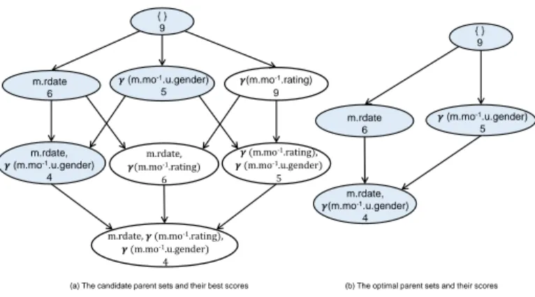
Theorem 7 Let U and S be two candidate parent sets for X.A such that U ⊂ S. We have BestScore(X.A | S) ≤ BestScore(X.A | U ).
Theorem 8 Let U and S be two candidate parent sets for X.A such that U ⊂ S, and Score(X.A | U) ≤ Score(X.A | S). Then S is not the optimal parent set of X.A for any candidate set.
We first apply Theorem 7 regarding score propagation to obtain our best scores. Then optimal parent sets are deduced according to Theorem 8. Figure 4.(a) shows the best scores corresponding to each candidate parent sets after scores’ propagation. The optimal parent sets and its best scores are depicted in Figure 4.(b). Then, as proposed in (Yuan and Malone, 2013), the optimal parent sets and their scores are sorted in two parallel lists: parentsX.A and scoresX.A. The best score of an
attribute X.A having all attributes as candidate parents, denoted BestScore(X.A | CPa(X.A)), is the first element in the sorted list. A heuristic proposed in (Malone, 2012) is then used to retreive any BestScore(X.A|S) from this list.
Example 5 Table 1 shows the sorted optimal scores of the descriptive attribute Movie.genre and their corresponding parents. BestScore(Movie.genre | CPa(Movie.genre)) is equal to 4, such as CPa(Movie.genre)∈ {γ(Movie.mo−1.rating); Movie.rdate;γ(Movie.mo−1.User.gender)}. If we
re-move both Movie.rdate andγ(Movie.mo−1.rating) from consideration, we scan the list from the be-ginning until finding a parent set that doesn’t include nor Movie.rdate neitherγ(Movie.mo−1.rating). That is equal to 9 in our example shown in Table 1.
3.3 The Relational Cost So Far
As in BN context, we define the cost so far of a node U in the relational order graph denoted by g(U ) as the sum of edge cost from the start node to U . We propose to define this cost, for each edge in the relational order graph connecting a node U to a node U ∪ {Xi.A} (where Xi.A is the added
attribute in the ordering) as follows :
(a) The candidate parent sets and their best scores (b) The optimal parent sets and their scores 𝜸(m.mo-1.rating) 9 𝜸 (m.mo-1.rating), 𝜸 (m.mo-1.u.gender) 5 m.rdate, 𝜸(m.mo-1.rating) 6 m.rdate, 𝜸 (m.mo-1.u.gender) 4 𝜸 (m.mo-1.u.gender) 5 m.rdate 6 { } 9
m.rdate, 𝜸 (m.mo-1.rating),
𝜸 (m.mo-1.u.gender) 4 { } 9 m.rdate 6 𝜸 (m.mo-1.u.gender) 5 m.rdate, 𝜸(m.mo-1.u.gender) 4
Figure 4: Score’ propagation and pruning in the relational parent graph of Movie.genre.
This formula corresponds to finding the best possible parent set for attribute Xi.A among the
attributes U already present in the model and A itself.
Example 6 The edge cost connecting Transaction.rating to Movie.genre is equal to BestScore(M ovie.genre | {CP ai/A(CP ai) ∈ (genre, rating)}). Referring to Table 1, this best score corresponds to the
first element that doesn’t contain the other attributes rdate and gender, i.e.BestScore(M ovie.Genre | γ(M ovie.mo−1.rating)) = 5. Thus the edge cost will be equal to 5.
3.4 The Relational Heuristic Function
The admissibility of the heuristic function h used in the BN context was proven in (Yuan et al., 2011). Accordingly we customize it to our relational extension, in equation 6 by also considering attributes that were not included yet in the ordering.
h(U ) =X
Xi
X
A∈A(Xi)\A(U )
BestScore(Xi.A | CP a(Xi.A)) (6)
Example 7 Let us compute h(M ovie.genre). The attributes not yet considered in the model are M ovie.rdate, U ser.gender and T ransaction.rating, so h(M ovie.genre) is equal to the sum over these 3 attributes of their best possible scores, respectively 5, 4 and 3 in Table 1, so h(M ovie.genre) = 5 + 4 + 3 = 12.
4. Toy Example
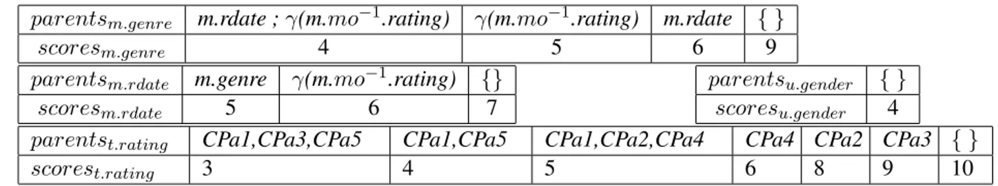
In this section, we illustrate the process of learning the optimal structure of a PRM through a toy example. We will apply the Relational BFHS using the A* search, which takes as input the relational order graph as a solution space and the optimal parent sets and their scores for each attribute of R. Our solution space is displayed in Figure 2. We assume, here, that the local scores have been computed for a complete instance of our relational schema. We have applied score’ propagation to the parent graphs of Movie.genre, Movie.rdate, User.gender and Transaction.rating and have kept the best scores and their corresponding optimal parents in Table 1.
parentsm.genre m.rdate ;γ(m.mo−1.rating) γ(m.mo−1.rating) m.rdate { }
scoresm.genre 4 5 6 9
parentsm.rdate m.genre γ(m.mo−1.rating) {}
scoresm.rdate 5 6 7
parentsu.gender { }
scoresu.gender 4
parentst.rating CPa1,CPa3,CPa5 CPa1,CPa5 CPa1,CPa2,CPa4 CPa4 CPa2 CPa3 { }
scorest.rating 3 4 5 6 8 9 10
Table 1: Sorted best scores and their corresponding parent sets for m.genre, m.rdate, u.gender and t.rating. CP a1 = t.u.gender, CP a2 = t.m.rdate, CP a3 = t.m.genre, CP a4 =
γ(t.u.us−1.rating) and CP a5= γ(t.m.mo−1.rating) denote the five candidate parents
of Transaction.rating.
Let us consider now our solution space and apply the A* search. Each node placed on the open or the closed list has the following form: (State, f, Parent), where State tells the set of attributes on the current node, f is equal to the sum of g-cost and h-cost and Parent reveals the set of attributes on the parent node. The algorithm starts with placing the start node on the open list. The start node contains the empty set. Obviously it has no parent and its evaluation function f ({}) is then equal to its heuristic function h({}). By definition, h is the sum of best possible scores for the attributes not yet considered, i.e. all the attributes in this step. Let’s denote BS1 = 4 the best score for M ovie.genre (first value in the corresponding array in Table 1), BS2 = 5 the best score for M ovie.rdate, BS3 = 4, the one for U ser.gender and BS4 = 3, the one for T ransaction.rating. Hence f ({}) = BS1 + BS2 + BS3 + BS4 = 16 and ({}, 16, void) is placed on the open list.
At the second iteration, ({}, 16, void) is placed on the closed list and its successors are generated. As shown in our relational order graph, successors of the start node are Movie.genre, Movie.rdate, User.gender and Transaction.rating. Let us consider Movie.rdate and Transaction.rating to illus-trate how to compute their evaluation functions.
Starting with Movie.rdate, the cost so far of that node is equal to the edge cost connecting the start node to that node. It is equal to BestScore(Movie.rdate | {}). Its value is retrieved from Table 1 and is equal to 7. h(Movie.rdate) is the sum of best possible scores for the attributes not yet considered. Hence, by using our previous notations, h(Movie.rdate) =BS1 + BS3 + BS4 = 11 and f(Movie.rdate) = 7 + 11 = 18.
In the same way, g(Transaction.rating)=BestScore(Transaction.rating | γ(Transaction.User.us−1.rating)) = 6 and h(Transaction.rating) is equal to BS1 + BS2 + BS3 = 13. Hence f(Transaction.rating)
= 19.
Similarly we compute the evaluation function of Movie.genre and User.gender. (User.gender,16,{}), (Movie.rdate,18,{}), (Transaction.rating,19,{}) and (Movie.genre,21,{}) are placed on the open list in the ascending order of their evaluation function. Then the first node having the minimum value of f in the open list is selected to be placed on the closed list and expanded. In our case, it will be (User.gender, 16,{}).
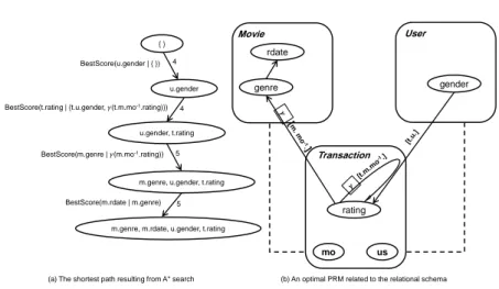
This process is repeated until the goal node is selected to be expanded. The shortest path is then defined by following backward to the start node. Figure 5.(a) displays the shortest path in our relational order graph resulting from applying A* search and Figure 5.(b) shows our optimal PRM deduced from that shortest path and the optimal parent sets.
{ }
m.genre, m.rdate, u.gender, t.rating u.gender
u.gender, t.rating
m.genre, u.gender, t.rating 4
4
5
5 BestScore(u.gender | { })
BestScore(t.rating | {t.u.gender, 𝛾(t.m.mo-1.rating)})
BestScore(m.genre |𝛾(m.mo-1.rating))
BestScore(m.rdate | m.genre) Movie Transaction User rdate genre rating gender mo us
(a) The shortest path resulting from A* search (b) An optimal PRM related to the relational schema
Figure 5: The shortest path in the relational order graph and the corresponding optimal PRM struc-ture.
5. Conclusion and Perspectives
In this paper, we have proposed an exact approach to learn optimal PRMs, adapting previous works dedicated to Bayesian networks (Malone, 2012; Yuan et al., 2011; Yuan and Malone, 2013) to the relational context. We have presented a formulation of our relational order graph, relational parent graph, relational cost so far and relational heuristic function. The BFHS can be then applied within our relational context.
Our relational order graph represents our solution space, where the BFHS is applied to find the shortest path and deduce then an optimal PRM. Our relational parent graph is used to find the optimal parent set for each attribute. This parent set depends on a given maximum slot chain length. We can also notice that one attribute may appear, potentially several times, on its own relational parent graph. By consequence, the cost so far g of an edge in our solution space, which corresponds to adding at least one edge between two attributes in our PRM, is also adapted to select the best parent set in this parent graph. The admissibility of the heuristic function h, inherited from the one proposed for Bayesian networks, guarantees that our Relational BFHS learns effectively the optimal structure of PRMs.
In the future, we plan to implement this approach to evaluate empirically its effectiveness, by using some optimizations proposed in (Malone, 2012). As a direct application of this work, we are also interested in developing an anytime PRM structure learning algorithm, following the ideas presented in (Aine et al., 2007; Malone and Yuan, 2013) for Bayesian networks.
References
S. Aine, P. P. Chakrabarti, and R. Kumar. AWA* - a window constrained anytime heuristic search algorithm. In M. M. Veloso, editor, IJCAI, pages 2250–2255, 2007.
M. Ben Ishak. Probabilistic relational models: learning and evaluation, the relational Bayesian networks case. PhD thesis, Nantes-Tunis, 2015.
X. Chen, T. Akutsu, T. Tamura, and W.-K. Ching. Finding optimal control policy in probabilistic boolean networks with hard constraints by using integer programming and dynamic program-ming. IJDMB, 7(3):321–343, 2013.
D. M. Chickering. Learning Bayesian networks is np-complete. Learning from data: Artificial intelligence and statistics v, pages 121–130, 1996.
G. F. Cooper and E. Herskovits. A Bayesian method for the induction of probabilistic networks from data. Machine Learning, 9:308–347, 1992.
J. Cussens. Bayesian network learning with cutting planes. CoRR, abs/1202.3713, 2012.
C. P. de Campos and Q. Ji. Efficient structure learning of Bayesian networks using constraints. Journal of Machine Learning Research, 12:663–689, 2011.
L. Getoor and B. Taskar, editors. Introduction to Statistical Relational Learning. The MIT Press, 2007.
L. Getoor, N. Friedman, D. Koller, and B. Taskar. Learning probabilistic models of relational struc-ture. In Proc. 18th International Conf. on Machine Learning, pages 170–177. Morgan Kaufmann, San Francisco, CA, 2001.
P. E. Hart, N. J. Nilsson, and B. Raphael. A formal basis for the heuristic determination of minimum cost paths. IEEE Transactions on Systems Science and Cybernetics, SSC-4(2):100–107, 1968. D. Koller and A. Pfeffer. Probabilistic frame-based systems. In J. Mostow and C. Rich, editors,
AAAI/IAAI, pages 580–587, 1998.
M. E. Maier, B. J. Taylor, H. Oktay, and D. Jensen. Learning causal models of relational domains. In M. Fox and D. Poole, editors, AAAI, 2010.
B. M. Malone. Learning Optimal Bayesian Networks with Heuristic Search. PhD thesis, Mississippi State University, Mississippi State, MS, USA, 2012.
B. M. Malone and C. Yuan. Evaluating anytime algorithms for learning optimal Bayesian networks. CoRR, abs/1309.6844, 2013.
J. Pearl. Heuristics: Intelligent Search Strategies for Computer Problem Solving. Addison & Wesley, 1984.
A. Pfeffer. Probabilistic reasoning for complex systems. PhD thesis, Stanford, 2000.
M. Teyssier and D. Koller. Ordering-based search: A simple and effective algorithm for learning Bayesian networks. CoRR, abs/1207.1429, 2012.
C. Yuan and B. M. Malone. Learning optimal Bayesian networks: A shortest path perspective. J. Artif. Intell. Res. (JAIR), 48:23–65, 2013.
C. Yuan, B. M. Malone, and X. Wu. Learning optimal Bayesian networks using A* search. In T. Walsh, editor, IJCAI, pages 2186–2191. IJCAI/AAAI, 2011.