HAL Id: hal-01007418
https://hal.archives-ouvertes.fr/hal-01007418
Submitted on 7 Nov 2018
HAL is a multi-disciplinary open access
archive for the deposit and dissemination of
sci-entific research documents, whether they are
pub-lished or not. The documents may come from
teaching and research institutions in France or
abroad, or from public or private research centers.
L’archive ouverte pluridisciplinaire HAL, est
destinée au dépôt et à la diffusion de documents
scientifiques de niveau recherche, publiés ou non,
émanant des établissements d’enseignement et de
recherche français ou étrangers, des laboratoires
publics ou privés.
Validation of a new 2D failure mechanism for the
stability analysis of a pressurized tunnel face in a
spatially varying sand
Guilhem Mollon, Kok Kwang Phoon, Daniel Dias, Abdul-Hamid Soubra
To cite this version:
Guilhem Mollon, Kok Kwang Phoon, Daniel Dias, Abdul-Hamid Soubra. Validation of a new 2D
failure mechanism for the stability analysis of a pressurized tunnel face in a spatially varying sand.
Journal of Engineering Mechanics - ASCE, American Society of Civil Engineers, 2011, 137 (1), pp.8-21.
�10.1061/(ASCE)EM.1943-7889.0000196�. �hal-01007418�
Validation
of a New 2D Failure Mechanism for the
Stability
Analysis of a Pressurized Tunnel Face in a Spatially
Varying
Sand
Guilhem
Mollon
1, Kok Kwang Phoon
2, Daniel Dias
3and Abdul-Hamid Soubra
4Abstract: A new two-dimensional 共2D兲 limit analysis failure mechanism is presented for the determination of the critical collapse
pressure of a pressurized tunnel face in the case of a soil exhibiting spatial variability in its shear strength parameters. The proposed failure mechanism is a rotational rigid block mechanism. It is constructed in such a manner to respect the normality condition of the limit analysis theory at every point of the velocity discontinuity surfaces taking into account the spatial variation of the soil angle of internal friction. Thus, the slip surfaces of the failure mechanism are not described by standard curves such as log-spirals. Indeed, they are determined point by point using a spatial discretization technique. Though the proposed mechanism is able to deal with frictional and cohesive soils, the present paper only focuses on sands. The mathematical formulation used for the generation of the failure mechanism is first detailed. The proposed kinematical approach is then presented and validated by comparison with numerical simulations. The present failure mechanism was shown to give results 共in terms of critical collapse pressure and shape of the collapse mechanism兲 that compare reasonably well with the numerical simulations at a significantly cheaper computational cost.
Author keywords: Tunnels; Active pressure; Limit analysis; Spatial variability; Local weakness.
Introduction
Stability is a key design/construction consideration in real shield tunnelling projects. The aim of stability analysis is to ensure safety against soil collapse in front of the tunnel face. This paper focuses on the study of the face stability of circular tunnels driven by pressurized shields in the case of a frictional soil. This study requires the determination of the minimal pressure 共air, slurry, or earth兲 required to prevent the collapse of the tunnel face.
The stability analysis of a pressurized tunnel face has been investigated by several writers in the literature. Some writers have performed experimental tests 共Chambon and Corté 1994; Takano et al. 2006兲. Others 共Horn 1961; Leca and Dormieux 1990; Eisen-stein and Ezzeldine 1994; Anagnostou and Kovari 1996; Broere 1998; Augarde et al. 2003; Klar et al. 2007兲 have studied the problem using analytical or numerical approaches. More recently, the face stability analysis was investigated by: 共1兲 Mollon et al.
共2009b, 2010兲 using the kinematical approach in limit analysis and 共2兲 Mollon et al. 共2009a兲 using numerical simulations as de-scribed below.
Mollon et al. 共2009b兲 suggested an analytical
three-dimensional 共3D兲 multiblock failure mechanism composed of several translational conical blocks, which improved the classical solutions by Leca and Dormieux 共1990兲 but presented the same shortcoming 共i.e., the mechanism was not able to deal with the entire circular tunnel face, but only with a vertical inscribed el-lipse兲. This shortcoming was solved in Mollon et al. 共2010兲, in which a new multiblock translational mechanism was presented which intersected the whole circular face. The construction of the slip surfaces of the different blocks was made point by point using a spatial discretization technique since no simple geometri-cal shape was able to intersect the whole tunnel face. Another approach was also proposed by Mollon et al. 共2009a兲 for the computation of the tunnel collapse pressure. These writers con-ducted 3D numerical simulations using the finite difference code FLAC3D 共Fast Lagrangian Analysis of Continua兲 共ITASCA Con-sulting Group 1993兲.
None of the above papers is related to spatially heterogeneous soils. Hence, the aim of this paper is to establish a suitable deter-ministic model that is able to deal with the spatial variation of the soil shear strength properties.
Fig. 1 presents the geometry of the problem considered in this paper. This study focuses on pressurized shields using com-pressed air as the retaining fluid. As a result, the applied face
pressure t is uniform. If this pressure drops below a critical
value 共critical collapse pressure c兲, the soil mass abutting the
tunnel face can collapse into the tunnel. In the case of a frictional
1
Ph.D. Student, INSA Lyon, Université de Lyon, LGCIE Site Cou-lomb 3, Géotechnique, Bât. J.C.A. CouCou-lomb, Domaine scientifique de la Doua, 69621 Villeurbanne cedex, France 共corresponding author兲. E-mail: Guilhem.Mollon@insa-lyon.fr
2
Professor, Dept. of Civil Engineering, National Univ. of Singapore, Singapore. E-mail: cvepkk@nus.edu.sg
3
Associate Professor, INSA Lyon, Université de Lyon, LGCIE Site Coulomb 3, Géotechnique, Bât. J.C.A. Coulomb, Domaine scientifique de la Doua, 69621 Villeurbanne cedex, France. E-mail: Daniel.Dias@insa-lyon.fr
4
Professor, Institut de Recherche en Génie Civil et Mécanique, Univ. of Nantes, UMR CNRS 6183, Bd. de l’université, BP 152, 44603 Saint-Nazaire cedex, France. E-mail: Abed.Soubra@univ-nantes.fr
soil, the arch effect can prevent this failure from reaching the ground surface, especially if the cover depth C is large enough with respect to the diameter D of the tunnel.
This paper proposes a new failure mechanism based on the kinematic theorem of limit analysis for the computation of the
critical collapse pressure c of a spatially varying soil. This
mechanism presents two main advantages for downstream sto-chastic analysis of the tunnel face: 共1兲 it is able to deal with spatial variations of the soil shear strength parameters and 共2兲 it is much less time-consuming than common numerical methods such as the finite-element method 共FEM兲 or the finite difference method 共FDM兲. However, this model has to be validated before using it in an extensive Monte Carlo simulation. This validation is done here by introducing some artificial weaknesses 共called “pix-els”兲 of several sizes and shapes systematically at several loca-tions in the soil mass. The impact of these weak pixels on the critical collapse pressure is studied. The same cases are treated with the commercial numerical software FLAC3D 共although a two-dimensional problem is involved in the present paper兲 in order to check that the proposed mechanism correctly accounts for these local shear strength weaknesses. The proposed mecha-nism can be applied to a general c- soil, but only analysis for purely frictional soils is presented herein.
It should be emphasized here that the present work is under-taken as part of a broader objective to study the impact of a spatially varying soil on the value of the critical collapse pressure
c. Realizations of spatially varying soil can be generated quite
readily using existing algorithms such as Karhunen-Loeve method and a Monte Carlo sampling method 共Phoon et al. 2005兲. Though reliable, this method requires a large number of calls of the deterministic model, which can be very time-consuming if one uses common numerical methods such as FEM or FDM. For instance, the numerical methods by Augarde et al. 共2003兲, Ukrichton et al. 共2003兲, Hjiaj et al. 共2005兲, Yamamoto et al. 共2009兲, and Abbo et al. 共2009兲 which successfully combined the FEM and the limit analysis theory for the study of stability prob-lems, both in undrained clays and in sands, are promising and can be used in the framework of a spatially varying soil. Notice, how-ever, that these methods are currently not quite practical for ex-tensive Monte-Carlo simulations because of the time cost of each call of the deterministic model. This time cost explains why the collapse mechanism presented in this paper is preferred for the stochastic analysis of pressurized tunnels.
The paper is organized as follows: first a description of the upper-bound approach in limit analysis and the proposed collapse
mechanism is presented. This is followed by the presentation of the numerical model using FLAC3D. Finally, the analytical and numerical results obtained in both cases of homogeneous and heterogeneous sands are presented and discussed.
Upper-Bound Theorem in Limit Analysis
The kinematic theorem in limit analysis is based on the work equation which states that the rate of external forces is equal to the rate of internal energy dissipation for a kinematically admis-sible velocity field respecting the flow rule and the velocity boundary conditions. For frictional soils, the validity of the upper-bound approach has been widely discussed in literature 共Chen and Liu 1990; Drescher and Detournay 1993; Soubra and Regenass 2000; Kumar 2004, among others兲. The assumption of an associ-ated flow rule for frictional soils is at the center of these discus-sions, because it is widely known from experimental tests that the dilation angle of sands is generally much smaller than the friction angle. However, this assumption is made in the framework of the kinematical theorem of limit analysis, since only for an associated material can the upper-bound theorem be proven true. For an associated flow rule material 共for which the velocity characteris-tics, i.e., the velocity discontinuities in a collapse mechanism, coincide with the stress characteristics often called “slip lines”兲, the angle between the slip line and the velocity vector should be equal to the soil angle of internal friction. In such a case, the plastic strain increment is normal to the failure criterion line in the Mohr-Coulomb plane 共and thus to the stress vector兲, and the stress vector at the velocity discontinuity has subsequently no dissipative effect 共Chen and Liu 1990; Drescher and Detournay 1993兲. The only energy dissipation in the system is related to cohesion, and the stresses in the soil mass are irrelevant to the solution. In the general case of nonassociated flow rule 共i.e.,
⫽兲, the velocity characteristics do not coincide with the stress
characteristics. The stresses are no longer normal to the strain increment, and therefore, they have a dissipating effect. In this case, two approximate 共not rigourous兲 kinematic analyses have been carried out in literature using the following expressions for the equivalent shear strength parameters共cⴱ, ⴱ兲 along the
veloc-ity characteristics as given by Davis 共1968兲:
cⴱ= c · cos · cos
1 − sin · sin 共1兲
tan ⴱ= cos · sin
1 − sin · sin 共2兲
The two kinematic analyses may be described as follows:
• For problems that do not require the determination of the
stress distribution along the velocity discontinuity surfaces to be solved by simple statics 共such as the case of a translational multiblock failure mechanism兲 and for which there is an equivalence between the force equilibrium equations and the energy balance equation, Drescher and Detournay 共1993兲 have shown that an approximate solution may be obtained by as-suming a fictitous 共cⴱ, ⴱ兲 soil with an associated flow rule
ⴱ= ⴱ. This is because in these cases, the energy balance
equation can be interpreted as an expression of the virtual rate of work principle and thus, an “apparent” energy balance equation can be used for the case of nonassociativeness by selection of a virtual velocity field that is not constrained by the flow rule. Since the limit load does not depend on the
orientation of the velocity jump, a “fictituous” orientation and
thus a fictituous flow rule 共ⴱ= ⴱ兲 has been selected by
Drescher and Detournay 共1993兲 for which the specific energy dissipation is independent of the normal stress distribution.
• For problems that do require the determination of the stress
distribution along the velocity discontinuity surfaces to be solved by simple statics, Kumar 共2004兲 have made an a priori assumption concerning this distribution using the results of the classical method of slices by Fellenius 共1936兲 and Bishop 共1955兲.
However, one should note that none of these two techniques is able to provide rigorous bounds of the critical load of a system. The assumption of an associated flow rule leads to clear results and clear limitations in the mathematical sense. The key task is to evaluate its limitations carefully with respect to the nonassociated flow rule nature of frictional soils. Finally, one should note that the present paper is not focusing on the exact determination of the critical collapse pressure of a tunnel face, but it deals with the effect of the spatial distribution of the friction angle in the soil when compared to the classical case of a uniform friction angle throughout the soil mass. This specific point will be closely in-vestigated in the next sections, by comparing the analytical results to the ones obtained by a numerical model with associated and nonassociated flow rules.
Collapse Mechanism
The limit analysis failure mechanism has to provide a correct approximation of the critical collapse pressure. It implies that the failure patterns of the mechanism should not be too different from the physical failures that can be observed during real tunnel face collapses.
Several writers undertook studies of tunnel face collapse on reduced models in frictional soils. Chambon and Corté 共1994兲 conducted their model tests in centrifuge, while the tests by Ta-kano et al. 共2006兲 were undertaken under 1 g. These writers re-ported that the failure pattern can be modeled by a rotational rigid-block failure mechanism and that the slip surfaces can be approximated by logarithmic spirals. This is in good agreement with the theory of limit analysis which states that a rotational failure in a frictional soil leads to a log-spiral slip surface in the case of a homogeneous soil 共i.e., a soil with a constant value of the angle of internal friction兲. Notice that, to our best knowledge, the mechanism in the presence of spatial variations of the soil shear strength parameters has not been studied yet. Therefore, there is a need to suggest a new failure mechanism that is able to take account of the spatial variations of the soil shear strength properties correctly. This problem is being addressed by the pro-posed two-dimensional 共2D兲 mechanism described below. As will be seen later, the slip surfaces of the rotational mechanism will not be described by log-spirals in the case of a spatially varying soil but rather by non standard curves that will be searched for point by point using a spatial discretization technique. The as-sumptions adopted in the analysis are listed below:
• Only the case of a cohesionless soil with an associated flow
rule is considered herein.
• For the sake of simplicity, it will be assumed that the failure
mechanism never outcrops, which is always true in practice as long as C ⬎ D where C and D = tunnel cover and diameter, respectively.
• The 2D failure mechanism intersects the tunnel face in two
points: A and B as shown in Fig. 2. Points A and B are
intro-duced here to cater to the possibility of local face collapse in the presence of strength heterogeneities.
• A rotational rigid block failure mechanism is assumed, O
being the rotation center.
The mechanism is described by four geometrical parameters as illustrated in Fig. 2. R and  are related to the position of the
center O of rotation, and H and Rmare related to the position of
the two points, A and B, where the mechanism intersects the
tunnel face; O⬘being the center of the tunnel face. In a
homoge-neous soil, the parameters H and Rm would be inapplicable
be-cause the mechanism would always intersect the whole tunnel face.
The failure mechanism should be kinematically admissible, which implies that the normality condition must be enforced at all points of the velocity discontinuity surfaces taking into account the spatial variation of the soil friction angle. The normality con-dition requires that the slip surface always makes an angle with the velocity vector V. If the friction angle is spatially varying,
then the slip surface at a point with coordinates共x , y兲 should be
searched for in such a manner to make an angle 共x , y兲 with the prescribed direction of the velocity vector V共x , y兲 at that point 共note that V共x , y兲 is normal to the corresponding radius兲, where 共x , y兲 and V共x , y兲 are the spatial distributions of the friction angle and velocity in the soil mass. As shown in Fig. 2, this geometrical condition implies that the slip surfaces emerging from A and B, respectively, are concave with respect to point O, and that these two lines will eventually meet in a point E which is the extremity of the mechanism. For a homogeneous frictional soil 共i.e., with a constant value throughout the soil mass兲, the normality condition would lead 共if the velocity field is a rigid-block rotation about point O兲 to a rigid rigid-block delimited by two logarithmic spirals, coming from points A and B, respectively, and terminating at point E which constitutes the extremity of the moving block. Such a mechanism would be easy to define ana-lytically, but would not be able to deal with a spatial variation of the friction angle of the soil, i.e., 共x , y兲.
To address the process of generation of the failure mechanism in the case of a spatially varying soil, an angular discretization
Fig. 2. Normality condition and geometric parameters共R ,  , H , Rm兲
scheme for the two curves emerging from A and B 共Fig. 3兲 was adopted. The generation process uses several radial lines meeting at the point of rotation, O. These lines are defined by an index j, with j = 0 corresponding to the first line OB. This set of sweeping lines with a common origin O terminates at line OE 共unknown a
priori兲. The angle ␦␣ between two successive radial lines is a
user-specified constant. The failure mechanism is divided into two sections. As shown in Fig. 3, Section 1 includes only the lower slip line, and Section 2 includes both the upper and the lower slip lines. The generation process aims at defining a collec-tion of points belonging to the two slip lines. Each point belong-ing to line j + 1 is defined from the previous point belongbelong-ing to line j, the whole process starting from points A and B for the
upper and lower slip lines, respectively. For example, point Bj+1
can be deduced from point Bjusing the two following conditions
共the same procedure is applied to deduce Aj+1from Aj兲:
• Bj+1belongs to line j + 1; and
• The straight segment BjBj+1 makes an angle 共Bj兲 with the
velocity vector v共Bj兲 at point Bj共note that the velocity vector
is normal to line j兲.
As a conclusion, for a spatially varying soil, the friction angle
to be considered at a given point Bjof a velocity discontinuity
surface is the local value of the friction angle at this point, called 共Bj兲. It is then straightforward to generate all the points Bj, from
Buntil the end of Section 1. For Section 2, the same method is
also used to generate points Aj+1and Bj+1from points Ajand Bj,
respectively. The upper and lower slip lines are generated until they cross at point E. With this generation process, the mecha-nism is constrained to respect the normality condition at each
point Ajand Bjof its contour. If the soil was homogeneous, the
two slip lines emerging from A and B could be analytically de-fined as logarithmic spirals, which equations would depend on 共1兲 the position of the center of rotation O and 共2兲 the two points A and B, i.e., the four geometrical parameters of the failure mecha-nism. Fig. 4 shows a plot of these analytical slip lines in a homo-geneous sand with = 30° where C = 10 m and D = 10 m, for a given set of the geometrical parameters of the failure mechanism. The contour points obtained by the discretization process de-scribed above are also plotted for two values of the angular
dis-cretization parameter ␦␣. It appears that this parameter should not
be larger than 1° if one wants to obtain a correct shape of the
mechanism, since the contour points for ␦␣= 5° are moving away
from the analytical slip lines. One may observe that the principle underlying the discretization process used herein is somewhat similar to the one presented in Mollon et al. 共2010兲. However, the proposed 2D failure mechanism is not a straightforward special case of the 3D mechanism studied previously because the present paper deals with a rotational mechanism which is more complex and more realistic than the translational mechanism presented in Mollon et al. 共2010兲. The writers believe that a 2D study is a necessary first step in the understanding of the behavior of a tunnel face in a spatially varying soil. Generalization of the present rotational mechanism to 3D may be developed in further studies.
The determination of the collapse pressure corresponding to this mechanism is based on the work equation, which states that the rate of work of the external forces applied to the moving soil mass is equal to the rate of energy dissipation. The applied forces to the moving block are: 共1兲 the weight of the soil composing the moving block; 共2兲 the collapse face pressure; and 共3兲 a possible surcharge loading on the ground surface in the case of outcrop of the mechanism 共not considered in the present study兲. The energy dissipation of the system takes place only at the velocity discon-tinuity surfaces in the present case of failure mechanism involv-ing rigid block movement. This energy dissipation is proportional to the cohesion 共Chen 1975兲. Since the cohesion is set to zero in the present paper, the energy dissipation is null. Finally, the work equation in the present case of a purely frictional soil with no surcharge loading becomes
W˙ + W␥ ˙ = 0c 共3兲
where
W˙c=
冕冕
⌺c· v . d⌺ 共4兲
Fig. 3. Principle of generation of the upper and lower slip lines of the failure mechanism
Fig. 4. Effect of the angular discretization parameter ␦␣on the con-tour points of the discretized failure mechanism in the case of a homogeneous soil and comparison with the exact analytical shapes 共i.e., log-spirals兲 of this mechanism
W˙␥=
冕冕
V
冕
␥· v · dV 共5兲
Computation of Eqs. 共4兲 and 共5兲 was performed numerically by discretizing the volume V of the moving block and the tunnel face surface ⌺ into elementary volumes and surfaces and by summa-tion of the corresponding elementary rates of work. This compu-tation may be explained with the aid of Fig. 5 as follows: the mechanism is first subdivided into several pseudoradial slices. In
Section 1, the slices are limited by two successive segments ABj
and ABj+1, and in Section 2 they are limited by two successive
segments AjBjand Aj+1Bj+1. Each segment j 关i.e., 共1兲 ABjor AB in
Section 1 and 共2兲 AjBj in Section 2兴 is subdivided into ni
seg-ments of equal length. Thus, niis the number of subdivisions of a
slice while njis the number of slices.
For the computation of the rate of work of the weight of an element Ci,jCi+1,jCi,j+1Ci+1,j+1共Fig. 5兲, this element is subdivided
into two triangles Ci,jCi,j+1Ci+1,j+1 and Ci,jCi+1,jCi+1,j+1 of
respec-tive barycenters Ci⬘,jand Ci⬙,j共Fig. 5兲. Thus, Eqs. 共4兲 and 共5兲 can be written in a discrete way as follows:
W˙ = −c
兺
i=1 ni c· Li,0· · Ri,0· sin共i,0兲 共6兲 W˙ =␥兺
j=1 nj兺
i=1 ni 关␥ · Si⬘,j· · Ri⬘,j· cos共i⬘,j兲 + ␥ · Si⬙,j· · Ri⬙,j· cos共i⬙,j兲兴 共7兲 where = angular velocity of the moving block; Li,0= length of anelementary segment Ci,0Ci+1,0 on the tunnel face; Ri,0= distance
between the middle point of segment Ci,0Ci+1,0 and point O; i,0
= inclination with the vertical of the velocity vector at the middle point of segment Ci,0Ci+1,0; Si⬘,j= area of triangle Ci,jCi,j+1Ci+1,j+1;
Si⬙,j= area of triangle Ci,jCi+1,jCi+1,j+1; Ri⬘,j= distance between Ci⬘,j
and point O; Ri⬙,j= distance between Ci⬙,j and point O; i⬘,j
= inclination with the vertical of the velocity vector at point Ci⬘,j; and i⬙,j= inclination with the vertical of the velocity vector at point Ci⬙,j. By solving Eq. 共3兲, one obtains the collapse pressure as follows: c= ␥ · D · N␥ 共8兲 N␥=
兺
j=1 nj兺
i=1 ni 关Si⬘,j· Ri⬘,j· cos共i⬘,j兲 + Si⬙,j· Ri⬙,j· cos共i⬙,j兲兴 D·兺
i=0 ni Li,0· Ri,0· sin共i,0兲 共9兲N␥= dimensionless parameter which depends on the size and
shape of the mechanism 共i.e., on the spatial distribution of the friction angle兲, and on the four geometrical parameters describing the mechanism 共Fig. 1兲. The collapse pressure defined by Eq. 共8兲 is a rigorous solution in the framework of the kinematical ap-proach of limit analysis. The best 共i.e., highest兲 solution that the
mechanism can provide is obtained by maximization of c with
respect to the four geometrical parameters of the failure mecha-nism. It should be emphasized here that the kinematic theorem allows the determination of an upper bound of the critical load. Since the face pressure is a force resisting collapse, it should be considered as a negative load. The best upper bound of this load
is therefore obtained by minimization of −c 共i.e., maximization
of c兲. When the soil is homogeneous, then the maximum is
unique. This fact has been observed by the writers of this paper and is consistent with the findings of other writers for different stability problems in geotechnical engineering. In this case, the
maximization of ccan be performed using a classical
optimisa-tion algorithm, such as the optimizaoptimisa-tion tools implemented in Matlab. The maximization procedure has produced in that case two logarithmic spirals curves 共results not shown兲. With a hetero-geneous soil, the optimization procedure has produced, as ex-pected, no log-spiral curves and the optimization was no longer possible using a classical optimization procedure because of the possible presence of local maximums for the collapse pressure. As an example, the left parts of Figs. 6共a and b兲 present two different response surfaces corresponding to two realizations of a random field of the friction angle. These response surfaces are plotted as lines of equal values of the critical collapse pressure in
the 共R , 兲 plane where the two parameters Rm and H are taken
equal to 5 and 0 m, respectively 共which corresponds to a full-face failure兲. In these figures, two successive solid lines are separated by 1 kPa and two successive dotted lines are separated by 0.05 kPa. On the right part of Figs. 6共a and b兲 are plotted the failure patterns corresponding to the global and local maximum values of
c. As one can see, several maximums can appear for a given
realization of a random field, making it impossible to use tradi-tional optimization methods such as the ones implemented in Matlab.
To obtain the global maximum, an exhaustive search over the full range of the four geometrical parameters was performed. The search for the global maximum was carried out in two steps. First, a coarse “grid” search was done as follows: 15° ⱕ  ⱕ 60° 共step: 2.5°兲; 3 m ⱕ R ⱕ 20 m 共step: 1 m兲; −1.5 m ⱕ H ⱕ 1.5 m 共step:
0.5 m兲; 3.5 m ⱕ Rmⱕ 5 m 共step: 0.5 m兲. Then, cwas computed
for all combinations of the four geometrical parameters and the biggest value of the collapse pressure was conserved. In a second step, the maximum found by using the coarse grid was employed as a starting point for a maximization process using an optimiza-tion tool provided by Matlab. This method ensures that the global maximum is found accurately. The two steps of the optimization process require about 4,000 calls of the model and the corre-sponding computation time was equal to 3 min 共with an angular
parameter ␦␣= 1°兲 when using a Core2 Quad CPU 2.4GHz PC.
More efficient optimization techniques such as the genetic
algo-Fig. 5. Principle of the discretization used to solve the work equation
rithm would be studied in the future in order to reduce the com-putation time.
Numerical Model
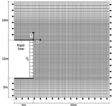
The numerical simulations presented in this study make use of the 2D numerical model shown in Fig. 7. These simulations are based on FLAC3D software although the problem is two-dimensional.
FLAC3D 共Fast Lagrangian Analysis of Continua兲 共ITASCA Consulting Group 1993兲 is a commercially available 3D finite difference code in which an explicit Lagrangian calculation scheme and a mixed discretization zoning technique are used. This code includes an internal programming option 共FISH兲 which enables the user to add his own subroutines. In this software, although a static 共i.e. nondynamic兲 mechanical analysis is re-quired, the equations of motion are used. The solution to a static problem is obtained through the damping of a dynamic process by including damping terms that gradually remove the kinetic energy from the system. A key parameter used in the software is the so-called “unbalanced force ratio.” It is defined at each calcula-tion step 共or cycle兲 as the average unbalanced mechanical force for all the grid points in the system divided by the average applied mechanical force for all these grid points. The system may be stable 共in a steady state of static equilibrium兲 or unstable 共in a
steady state of plastic flow兲. A steady state of static equilibrium is one for which 共1兲 a state of static equilibrium is achieved in the soil-structure system due to given service loads with constant values of the soil displacement 共i.e., vanishing values of the ve-locity兲 as the number of cycles increases and 共2兲 the unbalanced
force ratio becomes smaller than a prescribed tolerance 共e.g., 10−5
as suggested in FLAC3D software兲 as the number of cycles in-creases. On the other hand, a steady state of plastic flow is one for which soil failure is achieved. In this case, although the unbal-anced force ratio decreases as the number of cycles increases, this ratio does not go to zero but attains a quasi-constant nonvarying value. This value is usually higher than the one corresponding to the steady state of static equilibrium, but can be very small and still lead to infinite displacements, i.e., to failure.
In the model used in this study 共Fig. 7兲, the two vertical and the lower horizontal boundaries are assumed to be fixed in the normal direction. It was shown 共not detailed here兲 that this hy-pothesis leads to the same results as that for which the different boundaries are fixed on both the horizontal and the vertical direc-tions. The dimensions of the model are 25 m ⫻ 25 m. These di-mensions were adopted to ensure that the boundaries do not affect the critical collapse pressure 共not detailed here兲. The model is composed of 7,800 zones 共“zone” is the FLAC3D terminology for each discretized element兲 and approximately 16,000 grid points. The tunnel face is divided vertically into 40 zones.
The soil is assigned a perfect elastic-plastic constitutive model based on Mohr-Coulomb criterion with the elastic properties E = 240 MPa and = 0.22. These elastic properties do not have any significant impact on the critical collapse pressure. For this rea-son, a very high value of E was chosen because it increases the computation speed. Concerning the soil angle of internal friction and the soil dilatancy angle, their values are given later in the paper. The upper and lower lining of the tunnel are modeled as linear elastic. Their elastic properties are Young’s modulus E = 15 GPa and Poisson’s ratio = 0.2. The lining is connected to the soil via interface elements that follow Coulomb’s law. The interface is assumed to have a friction angle equal to two thirds of the soil angle of internal friction and no cohesion. Normal
stiff-Fig. 6. Response surface of the collapse pressure in the共 , R兲 plane in the case of two random distributions of 共left兲 and corresponding failure mechanisms in the random soil 共dark areas correspond to low values and bright areas correspond to high values兲 corresponding to the different maximums
Fig. 7. 2D numerical model used for the determination of the critical collapse pressure using FLAC3D software
ness Kn= 1011 Pa/ m and shear stiffness K
s= 1011 Pa/ m were
as-signed to this interface. These parameters are functions of the neighboring elements rigidity 共ITASCA Consulting Group 1993兲. They have almost no influence on the collapse pressure.
The fastest method for the determination of the critical col-lapse pressure would be a strain-controlled method but it is diffi-cult to apply for stability analysis of tunnels because it assumes that the deflected shape of the tunnel face is known. This shape is not known a priori and any assumption 共such as uniform or para-bolic deflection兲 may lead to errors in the determination of the collapse pressure. Thus, a stress-controlled method is used herein. A simple approach would consist of successively applying de-creasingly prescribed uniform pressures on the tunnel face until failure occurs. Of course, this requires a significant number of numerical simulations to obtain a satisfactory value of the critical collapse pressure which is very time-consuming. A more rational approach called the bisection method is suggested in this paper and coded in FISH language. It allows the critical collapse pres-sure of the tunnel face to be determined within an accuracy of 0.1 kPa, and is detailed below.
• The initial lower bracket corresponds to any trial pressure for
which the system is unstable. This state corresponds to a non-zero face extrusion velocity 共i.e., an infinite displacement兲 at each point of the tunnel face and means that a steady state of failure or plastic flow is achieved in this case. From a compu-tational point of view, the system is considered as unstable if the tunnel face extrusion continues to increase 共the velocity of this extrusion remaining almost constant兲 after 40,000 compu-tation cycles. Notice that the unbalanced force ratio adopted in
this paper is 10−7 since the value of 10−5 suggested in
FLAC3D software was shown not to give an optimal solution in the present case. The choice of 40,000 for the number of cycles has been determined after several trials: it is large enough to ensure that the system will never be stable if it is still unstable after running these 40,000 cycles.
• The initial upper bracket corresponds to any trial pressure for
which the system is stable. This state corresponds to a zero face extrusion velocity 共i.e., a constant displacement兲 at each point of the tunnel face and means that a steady state of static equilibrium is achieved in that case. The system is considered
as stable when the unbalanced force ratio drops under 10−7
before 40,000 computation cycles.
• Next, a new value, midway between the upper and lower
brackets, is tested. If the system is stable for this midway value, the upper bracket is replaced by this trial pressure. If the system does not reach equilibrium, the lower bracket is then replaced by the midway value.
• The previous step is repeated until the difference between
upper and lower brackets is less than a prescribed tolerance, namely 0.1 kPa in this study. Since the width of the interval is divided by two at each step, a convenient method might be to use a first interval with a width equal to n times 0.1 kPa, n being a power of two.
Validation of the Proposed Mechanism in Homogeneous Sands
The validity of the proposed mechanism in homogeneous sands is evaluated in this section through a comparison with the numerical model. This comparison is done over the whole range of typical friction angles for sands 共i.e., from 30° to 45°兲, considering a
tunnel with D = 10 m and a soil with ␥ = 18 kN/ m3. Two cases
will be studied in the numerical model: the first one with an
associated flow rule共 = 兲 and the second one with zero angle of
dilatancy共 = 0兲. It is believed that the plastic behavior of a real sand is somewhere between these two limit cases. As is well known, numerical models 共e.g., FEM, FDM兲 can easily handle nondilatant behaviors of the soil with a nonassociated flow rule 共De Borst 1991; Loukidis and Salgado 2009, among others兲. The question of whether the numerical problem is even well posed in the case of nonassociated flow is worthy of a brief mention here, since issues related to nonassociated plasticity are not completely resolved in literature.
The results in terms of failure pattern and collapse pressure are
given in Figs. 8 and 9. Notice that only the 共 = 兲 case is
con-sidered in Fig. 8 since the limit analysis assumes an associated flow rule material. The discretization parameter used for the limit
analysis mechanism was ␦␣= 1°. The computation time was about
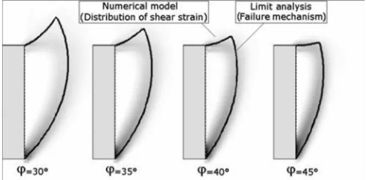
3 min for the limit analysis model and 120 min for the numerical model, both on a Core2 Quad CPU 2.40GHz. This illustrates the claim that the proposed limit analysis model is much more time efficient and hence, more practical for stochastic simulation. Fig. 8 shows the most critical slip lines provided by limit analysis as well as the corresponding plastic shear strain patterns provided by the numerical model for several values of . There is a reasonably
Fig. 8. Slip lines provided by limit analysis and corresponding dis-tributions of plastic shear strain provided by the numerical model in the case of a homogeneous sand
Fig. 9. Comparison between the critical collapse pressures provided by limit analysis and by the numerical model for = and = 0 in the case of a homogeneous sand
good agreement between the two approaches. Fig. 9 presents the
cvalues provided by limit analysis and by the numerical model
共for both = and = 0兲 for different values. The impact of the assumption of associated flow rule clearly appears on this figure. The fact of considering = instead of = 0 reduces the critical collapse pressure by 8% when = 30° and by 21% when = 45°. The case = 0 should not be regarded as the real case but as an extreme limit case, because nonzero values of the dilation angle are likely to appear, especially for high friction angles. The ana-lytical curve shows good qualitative agreement in terms of the trend. However, an anomaly should be pointed out. Though the proposed kinematical approach is known to provide a rigorous solution and this solution is expected to be lower 共this is because the tunnel pressure resists collapse兲 than the exact one in the framework of limit analysis, the present mechanism was shown 共Fig. 9兲 to give higher values of the pressure than the numerical model for = 共associated flow rule兲. This anomaly may be due to the chosen mesh as explained below.
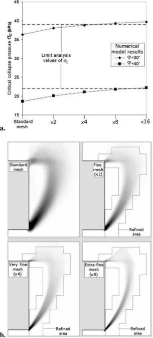
The distributions of the plastic shear strain provided by the numerical model and shown in Fig. 8 appear to be quite spread out when compared to the limit analysis mechanism, which is based on velocity discontinuity surfaces. It should be noted that Chambon and Corté 共1994兲 and Takano et al. 共2006兲 have pointed out a sudden discontinuity in the velocity when they performed their experimental model tests. Hence, the sudden discontinuity used in limit analysis model seems to really reflect the observed sudden collapse phenomenon in sands. The smearing of the shear strain zone given by the numerical model may therefore be inter-preted as an effect of the numerical simulation. The obvious cause of smearing is probably the coarseness of the mesh, which gov-erns the velocity gradient. To study this issue, several numerical simulations were realized with locally refined meshes. The refined area was chosen so as to cover all the zones of the mesh with a likely high velocity gradient 共i.e., in the vicinity of the velocity discontinuity surfaces obtained from limit analysis兲, and is illus-trated in Fig. 10共a兲. Different meshes were selected, with progres-sive local refinement, as presented in Fig. 10共b兲. The so-called “standard mesh” is similar to the one used earlier in this paper. The critical collapse pressure of the tunnel was calculated for each of these meshes, in the case of an associated flow rule and for two different values of the friction angle 共 = 30° and = 40°兲, using the bisection method detailed earlier. Fig. 11共a兲 pre-sents the numerical results of this study. It clearly shows that a refined mesh in the zones of high velocity gradients increases the value of the critical collapse pressure with respect to the standard mesh and makes it much more consistent with the results of the limit analysis mechanism 共both for = 30° and = 40°兲. It is how-ever necessary to refine the mesh significantly 共by a factor 16兲 for the anomaly pointed out earlier to vanish for both friction angles. Concerning the failure pattern, the local refinement of the mesh makes the distribution of the plastic shear strain much more “con-centrated” as shown in Fig. 11共b兲. A velocity discontinuity is not expected to appear in the numerical model even for an extremely fine mesh, since the concept of discontinuity does not exist in a continuum formulation like the finite difference method. How-ever, the reduction of the width of the shear zone 共induced by mesh refinement兲 increases the gradient of velocity in this zone, and thus makes it closer to the infinite velocity gradient postu-lated by the analytical model. This is in good agreement with De Borst 共1991兲, who demonstrated that when simulating numeri-cally the shear deformations in a frictional soil submitted to a biaxial-compression test, the width of the shear band was closely related to the coarseness of the mesh. This width was found to
remain between one and two times the size of a mesh element. It was also found that the coarseness had an impact on the critical pressure, and that a refinement of the mesh led to closer agree-ment with limit analysis. Thus, the numerical model with a so-called “extra-fine mesh” 共i.e., a size of the FLAC3D zone reduced by a factor eight兲 provides a correct value for the critical collapse pressure and a significant improvement in the shape of the failure, but one should notice that this improvement has a price. The computation time with this model is about 30 times longer than that for the standard mesh, which significantly limits its use in parametric studies or in stochastic simulations. The coarseness of the mesh in the vicinity of high velocity gradients therefore ap-pears to have a significant effect on the results 共i.e., on the critical pressure and the corresponding failure pattern兲 of a numerical simulation. For this reason, two different kinds of meshes will be used from hereon.
• For studies involving a large number of simulations, the
stan-dard mesh of the numerical model will be used for the valida-tion of the proposed limit analysis model because it appears to reproduce qualitative trends with reasonable accuracy. When
Fig. 10. Locally refined meshes: 共a兲 localization of the refined area; 共b兲 details of the four meshes at the invert of the tunnel face
dealing with this standard mesh, all the subsequent results relative to the introduction of a local weakness will be pre-sented in percent increase with respect to the homogeneous case since it is the most relevant way to express the effect of an heterogeneity; the values provided, in the homogeneous case, by both the standard mesh of the numerical model and by the proposed limit analysis method being quite different.
• If more accurate results on the shape of failure and the critical
collapse pressure are needed, a locally refined mesh will be used. This mesh will be similar to the “extra-fine” mesh pre-sented earlier, except that the refined area will be adjusted appropriately to cover the expected shear zone of the corre-sponding simulation.
Validation of the Proposed Mechanism in Heterogeneous Sands
The proposed mechanism has been proven to be suitable for ho-mogeneous sands. However, more advanced validations are needed to cover cases of spatially varying sands, which would appear in random field simulations. Two cases were studied: the first one involves a systematic study of the impact of a local weakness in the soil on the critical collapse pressure and the corresponding failure pattern. This study is done by introducing a so-called weak pixel in the soil mass. This pixel may have differ-ent locations, sizes and shapes 共i.e., square pixel, horizontal layer or vertical layer兲. The second case considers a real spatially vary-ing soil. Both cases are detailed in the two followvary-ing sections. Case of a Local Weakness in the Soil Mass
For a given simulation, the friction angle remains constant outside of the weak pixel, and is decreased by a given percentage inside the pixel. Each case is dealt with using the proposed mechanism and the numerical model 共for both = and = 0兲.
Validation in Terms of Collapse Pressures
Fig. 12 shows the percent increase in the critical collapse pressure as given by limit analysis and by the numerical model in the case where a 2-m square weak pixel located at the invert of the tunnel face is considered in the analysis. As explained before, the results are presented herein in percent increase with respect to the homo-geneous case. The friction angle is reduced by 20% inside the pixel, and the values of outside the pixel cover the usual range of sands 共i.e., 30° ⬍ ⬍ 45°兲. Two limit values of the dilatancy angle are considered in the analysis. The conclusions concerning the results obtained in the present case are very similar to those provided in the homogeneous soil case, i.e., there is a satisfying agreement 共the maximal difference is equal to 5%兲 between limit analysis and the numerical model 共both for associated and nonas-sociated rule兲 when the error induced by the coarseness of the standard mesh of the numerical model is evacuated through the
use of a percent increase in c with respect to the homogeneous
case. Moreover, the two numerical curves for associated and
non-Fig. 11. Effect of mesh local refinement on: 共a兲 critical collapse pressure for = 30° and = 40°; 共b兲 distributions of plastic shear strain for = 30°
Fig. 12. Percent increase in the critical collapse pressure due to a reduction of by 20% in a 2-m square pixel at the invert of the tunnel face
dilatant soils appear to be quite similar 共less than 3% of differ-ence兲. This observation 共confirmed by the Figs. 13–15 later in this paper兲 provides an indication of the significance of our study with respect to the associated flow rule limitation highlighted above. As expected, the assumption of associated flow rule can introduce
a systematic error in the determination of cas shown in Fig. 9.
However, this assumption affects the relative increase of c
in-duced by a local weakness in a limited way. In other words, flow rule affects the absolute value of c, but hardly affects the relative
change in c, which is the primary goal in this paper.
Fig. 13 shows a more systematic study concerning the impact of the position of a local weakness. In this figure, only a 2-m square pixel with a local reduction of by 20% is considered. The friction angle outside of the pixel is equal to 30° 共i.e., the friction angle inside the weak pixel is equal to 24°兲. All the po-sitions of the pixel around the tunnel face are tested and the
critical collapse pressures are computed using both the proposed mechanism and the numerical model 共for both = and = 0兲. Due to the high number of simulations, the standard mesh was
used in the numerical model and the percent increase in cwith
respect to the homogeneous case is presented. Fig. 13 therefore presents for each pixel 共shade of gray and numerical value兲 the
percent increase in c caused by a 20% reduction of in this
pixel. The three models provide quite similar results for the
in-crease of c, which means that: 共1兲 although the dilatancy angle
has an effect on the value of c, it has almost no effect on the
relative increase of the tunnel collapse pressure in the presence of a local weakness and 共2兲 the proposed failure mechanism gives consistent results with the numerical model when dealing with a local reduction of . The numerical results also show that a local weakness at the invert of the tunnel face has an important impact
on the stability, the increase in c being larger than 10% with
respect to the homogeneous case. A local weakness at the crown
Fig. 13. Percent increase in the critical collapse pressure due to a reduction of by 20% in a 2-m square pixel for several locations of this pixel in the soil mass 共a white pixel means no impact of this pixel on the face stability兲
Fig. 14. Impact of a decrease in the soil friction angle on c for a
pixel located at the invert of the tunnel face for several sizes of the weak pixel
Fig. 15. Percent increase in the critical collapse pressure due to a reduction of by 20% in a 2m-thick weak layer for several locations of this layer in the soil mass in the case of 共a兲 horizontal weak layer; 共b兲 vertical weak layer
of the tunnel face does influence the critical collapse pressure but this influence is much smaller than that at the invert. The central part of the tunnel face appears to have a negligible effect on the face stability. The most critical zone for the tunnel face stability is therefore located at the invert of the tunnel face, and it seems to have a significant impact on the critical collapse pressure com-pared to the other parts of the tunnel face.
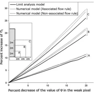
The impact of a local decrease of a pixel’s friction angle on the tunnel collapse pressure in the case of a pixel located at the tunnel invert is plotted in Fig. 14. It is expressed in terms of a percent increase in the tunnel collapse pressure with respect to the homo-geneous case. Three sizes of the weak pixel named Cases A, B, and C and corresponding, respectively, to 2, 4, and 6-m square pixels are used in the analysis. The friction angle outside of the pixel remains equal to 30°. In the present case, the numerical model makes use of the standard mesh. Once again, the proposed mechanism shows a satisfying agreement with the results of the numerical model, both for associated and nonassociated sands. The critical collapse pressure appears to increase linearly with the local decrease of for the three sizes of pixels. Moreover, the impact of the local weakness increases with the size of the pixel:
a local reduction of by 20% leads to an increase in cby 10.6,
19.3, and 26.0% for Cases A, B, and C, respectively.
A similar study was carried out with a weak layer instead of a weak pixel. A horizontal and a vertical layer with a thickness equal to 2 m were considered in the analysis. A vertical layer is clearly not likely to appear in a real soil 共though not impossible兲, but is used here to study the impact of a local weakness which would be more extended in the vertical direction than in the hori-zontal one. Both vertical and horihori-zontal weaknesses can appear in an isotropic random field due to fortuitous aggregation and align-ment of weak spots in a preferred direction. We expect vertical weakness to be more critical and hence it is included in this study.
In Fig. 15共a兲, the percent increase in c due to a 2m-thick
hori-zontal weak layer was plotted with respect to the y-coordinate of the center of this weak layer. Similarly, Fig. 15共b兲 presents the
percent increase in cdue to a 2-m thick vertical weak layer with
respect to the x-coordinate of the center of this weak layer. The reduction of in the horizontal and vertical layers is equal to 20%, and the value of outside the weak layer is 30°. The pro-posed kinematical approach gives correct results when compared to the numerical model for both cases of a horizontal or a vertical layer, which confirms the observations of the previous paragraph. The most critical horizontal layer is the one located at the invert
of the tunnel face, and the corresponding increase in cis larger
than 10% with respect to the homogeneous case. As expected, a vertical layer has a larger impact on the stability; probably be-cause the shape of failure is mainly vertical 共i.e., the slip lines of the failure mechanism are following directions that are not far from the vertical兲. A 2-m thick vertical layer which center is
lo-cated between 2 m and 4 m behind the tunnel face can increase c
by more than 20%.
Validation in Terms of Failure Patterns
Only the most relevant cases where the soil heterogeneity may have an effect on the failure pattern are plotted in Fig. 16. Cases 共a兲 and 共b兲 correspond to 4-m square weak pixels located, respec-tively, at the invert and at the crown of the tunnel, and Cases 共c兲 and 共d兲 correspond to 2-m thick vertical layers located at two different distances from the tunnel face. The reduction of in the weak pixels or layers remains at 20% and the friction angle out-side the pixels or layers is taken equal to 30°. The failure patterns provided by both the limit analysis failure mechanism and by the
numerical model 共with the so-called extra-fine mesh兲 are pre-sented in Fig. 16. They show reasonable agreement. For Case 共a兲, the shape of the failure pattern does not differ significantly from that of the homogeneous case. For Case 共b兲, the mechanism is stretched vertically in the weak pixel located at the crown of the tunnel face. Cases 共c兲 and 共d兲 show that the vertical weak layers can “attract” the failure mechanism much more than the weak square pixels because the lower slip line of the mechanism is aligned in a predominantly vertical direction. Based on this ob-servation, one can postulate that an “inclined” layer at the invert of the tunnel face would probably be the most critical shape for a local weakness, because it would be located in the most critical area 共invert of the face兲 and would “fit” the lower slip line even better than a vertical layer.
Case of a Random Soil
The validation of the failure mechanism in spatially varying soils is undertaken in this section. Two 2D random fields of the friction angle were generated using Karhunen-Loeve expansion method 共Phoon et al. 2005兲 and were applied to the limit analysis model and to the numerical model 共with the extra-fine mesh兲. The two fields are lognormal spatial distributions of with a mean value log= 30° and a standard deviation log= 3° 共i.e., a coefficient of
variation COV of 10%兲. To generate such a field with the Karhunen-Loeve expansion method, one first has to generate a
normal random field with a mean value normal and a standard
deviation normal. The first two moments of this underlying normal
field can be obtained by using the target moments of the lognor-mal random field 共logand log兲 as follows:
normal=
冑
ln冉
1 + log2 log2冊
共10兲 normal= ln共log兲 + 1 2· normal 2 共11兲The underlying normal fields are assumed to follow an exponen-tial autocorrelation function, i.e., the coefficient of correlation be-tween two points, A and B, can be obtained by the following expression 共Sudret and Der Kiureghian 2000兲:
共A,B兲 = exp
冉
−兩xA− xB兩Lx
−兩yA− yB兩
Ly
冊
共12兲 In the present paper, only isotropic random fields 共i.e., where the
autocorrelation lengths Lx and Ly are such that Lx= Ly= L兲 are
Fig. 16. Failure patterns provided by the proposed failure mecha-nism and by the numerical model 共with an extra fine mesh兲 for sev-eral shapes and positions of the local weakness in the soil mass and comparison with the failure mechanism of a homogeneous soil
considered in the analysis. It can be demonstrated that, as long as the coefficient of variation of the random field remains small 共which is the case when dealing with the friction angle兲, the au-tocorrelation function of the lognormal field is very similar to the one of the underlying normal field 共Sudret and Der Kiureghian 2000兲. The two lognormal random fields used in the present stud-ies are therefore considered to follow the autocorrelation function given by Eq. 共12兲, with respective autocorrelation lengths of L = 1 m and L = 5 m.
The left parts of Figs. 17共a and b兲 show the two random fields around the tunnel face 共the dark areas correspond to low friction angles and the light areas correspond to high friction angles兲. The
numerical model and the proposed limit analysis approach pro-duce comparable results in terms of the collapse pressure. The failure patterns provided by the proposed failure mechanism and by the numerical model for the two random soils are compared on the right part of Figs. 17共a and b兲. The slip lines appear less “regular” than in the homogeneous case because of the spatial variation of the friction angle and subsequently of the local value of the angle of internal friction that should exist at each point of the slip lines between the slip line and the velocity vector. The failure mechanisms and the corresponding collapse pressures pro-vided by the two models are very similar for both random fields, which imply that the proposed limit analysis approach can be
Fig. 17. Random fields of the friction angle for two values of the autocorrelation distance 共left兲, resulting failure patterns provided by the numerical model and by the proposed failure mechanism 共right兲 and comparison with the failure mechanism of a homogeneous soil 共center兲
used with confidence for downstream stochastic simulations. Field 1 leads to a relatively smaller and vertical failure zone, while Field 2 leads to a more extended failure in the horizontal direction. Such an observation based on only two samples is ob-viously tentative and will have to be confirmed by an extensive Monte-Carlo simulation. This topic will be the subject of future studies.
Finally, the failure patterns and the corresponding collapse pressures obtained by the proposed failure mechanism in both the homogeneous soil and the spatially varying soil are presented in the central part of Figs. 17共a and b兲. It appears that there is no direct relationship between the size and shape of the mechanism and the critical collapse pressure for a given sample of the ran-dom field.
Conclusions
This paper aimed at presenting and validating a new 2D failure mechanism for the determination of the critical collapse pressure of a pressurized tunnel face in the case of a sand layer exhibiting several types of weaknesses 关共1兲 a local weakness represented by a weak pixel or a weak layer or 共2兲 a more general case of weak-ness concerning a random soil represented by an autocorrelation function兴. Validation is carried out by comparison with 2D nu-merical model using the commercial software FLAC3D. The pro-posed kinematical approach provides consistent results both in terms of the collapse pressure and the failure pattern when com-pared to the numerical model, and can therefore be used with confidence in soils modeled as random fields. Moreover, the as-sumption of associated flow rule used in the analytical model was tested with the numerical model. It appeared that this assumption leads to a systematic underestimation of the critical collapse pres-sure 共from 8 to 21% for the common values of in a sand with respect to the limit case = 0兲, but has very little impact when dealing with the relative change of the critical pressure from a homogeneous to a spatially heterogeneous distribution of .
The systematic study of the impact of local weaknesses 共weak pixels or weak layers兲 on the face stability has demonstrated that the most critical weakness area is the one located at the invert of the tunnel face.
This study has two important ramifications. First, the discreti-zation technique used for the generation of the failure mechanism can also be used to compute the failure load or the safety factor in spatially varying soils relevant to other stability problems in geo-technical engineering, such as footings and slopes. Second, the significant computational savings would bring Monte Carlo simu-lations of random field problems 共basically all stability problems in geotechnical engineering兲 within reach of the average practi-tioner using modest computing platforms. Current random finite element methods based on Monte Carlo simulations are too te-dious to be applied to routine problems in practice.
Acknowledgments
This research was carried out during a stay of the first writer in the Department of Civil Engineering at the National University of Singapore from March to September 2009, with the permission and financial support of the LGCIE 共Laboratoire de Génie Civil et d’Ingénierie Environementale, INSA Lyon, Université de Lyon, France兲. These two institutions are gratefully acknowledged.
References
Abbo, A. J., Wilson, D. W., Lyamin, A. V., and Sloan, S. W. 共2009兲. “Undrained stability of a circular tunnel.” Proc., EURO:TUN 2009
Congress, Aedificatio Publishers, Freiburg, Germany, 857–864. Anagnostou, G., and Kovari, K. 共1996兲. “Face stability conditions with
earth-pressure-balanced shields.” Tunn. Undergr. Space Technol., 11共2兲, 165–173.
Augarde, C. E., Lyamin, A. V., and Sloan, S. W. 共2003兲. “Stability of an undrained plane strain heading revisited.” Comput. Geotech., 30, 419–430.
Bishop, A. W. 共1955兲. “The use of slip-circle in the stability analysis of slopes.” Geotechnique, 5共1兲, 7–17.
Broere, W. 共1998兲. “Face stability calculation for a slurry shield in het-erogeneous soft soils.” Proc., World Tunnel Congress 98 on Tunnels
and Metropolises, Vol. 1, Balkema, Rotterdam, The Netherlands, 215– 218.
Chambon, P., and Corté, J. F. 共1994兲. “Shallow tunnels in cohesionless soil: Stability of tunnel face.” J. Geotech. Engrg., 120共7兲, 1148–1165. Chen, W. F. 共1975兲. Limit analysis and soil plasticity, Elsevier,
Amster-dam, The Netherlands.
Chen, W. F., and Liu, X. L. 共1990兲. Limit analysis in soil mechanics, Elsevier Science, Amsterdam, The Netherlands.
Davis, E. H. 共1968兲. “Theories of plasticity and the failure of soil masses.” Soil mechanics: Selected topics, I. K. Lee, ed., Butterworth, London, 341–380.
De Borst, R. 共1991兲. “Numerical modelling of bifurcation and localisa-tion in cohesive-friclocalisa-tional materials.” Pure Appl. Geophys., 137共4兲, 367–390.
Drescher, A., and Detournay, E. 共1993兲. “Limit load in translational fail-ure mechanisms for associated and non-associated materials.”
Geo-technique, 43共3兲, 443–456.
Eisenstein, A. R., and Ezzeldine, O. 共1994兲. “The role of face pressure for shields with positive ground control.” Tunneling and ground
condi-tions, Balkema, Rotterdam, The Netherlands, 557–571.
Fellenius, W. 共1936兲. “Calculation of stability of earth dams.” Proc.,
Transactions 2nd Congress on Large Dams, Vol. 4, International Commission on Large Dams, Washington, D.C.
Hjiaj, M., Lyamin, A. V., and Sloan, S. W. 共2005兲. “Numerical limit analysis solutions for the bearing capacity factor N␥.” Int. J. Solids
Struct., 42, 1681–1704.
Horn, N. 共1961兲. “Horizontaler erddruck auf senkrechte abschlussflächen von tunnelröhren.” Landeskonferenz der ungarischen tiefbauindustrie, Deutsche Überarbeitung durch STUVA, Düsseldorf, 7–16.
ITASCA Consulting Group. 共1993兲. FLAC3D: Fast Lagrangian analysis
of continua, Minneapolis.
Klar, A., Osman, A. S., and Bolton, M. 共2007兲. “2D and 3D upper bound solutions for tunnel excavation using ‘elastic’ flow fields.” Int. J.
Numer. Analyt. Meth. Geomech., 31共12兲, 1367–1374.
Kumar, J. 共2004兲. “Stability factors for slopes with non-associated flow rule using energy considerations.” Int. J. Geomech., 4共4兲, 264–272. Leca, E., and Dormieux, L. 共1990兲. “Upper and lower bound solutions for
the face stability of shallow circular tunnels in frictional material.”
Geotechnique, 40共4兲, 581–606.
Loukidis, D., and Salgado, R. 共2009兲. “Bearing capacity of strip and circular footings in sand using finite elements.” Comput. Geotech.,
36共5兲, 871–879.
Mollon, G., Dias, D., and Soubra, A.-H. 共2009a兲. “Probabilistic analysis of circular tunnels in homogeneous soils using response surface meth-odology.” J. Geotech. Geoenviron. Eng., 135共9兲, 1314–1325. Mollon, G., Dias, D., and Soubra, A.-H. 共2009b兲. “Probabilistic analysis
and design of circular tunnels against face stability.” Int. J. Geomech., 9共6兲, 237–249.
Mollon, G., Dias, D., and Soubra, A.-H. 共2010兲. “Face stability analysis of circular tunnels driven by a pressurized shield.” J. Geotech.
Geoen-viron. Eng., 136共1兲, 215–229.
strongly non-Gaussian processes using Karhunen-Loeve expansion.”
Probab. Eng. Mech., 20共2兲, 188–198.
Soubra, A.-H., and Regenass, P. 共2000兲. “Three-dimensional passive earth pressures by kinematical approach.” J. Geotech. Geoenviron. Eng.,
126共11兲, 969–978.
Sudret, B., and Der Kiureghian, A. 共2000兲. “Stochastic finite element methods and reliability, a state of the art.” Rep. No.
UCB/SEMM-2000/08, Dept. of Civil and Environmental Engineering, Univ. of California, Berkeley, Berkeley, Calif.
Takano, D., Otani, J., Nagatani, H., and Mukunoki, T. 共2006兲.
“Applica-tion of X-ray CT boundary value problems in geotechnical engineering—Research on tunnel face failure.” Proc., Geocongress, ASCE, Reston, Va., 1–6.
Ukrichton, B., Whittle, A. J., and Klangvijit, C. 共2003兲. “Calculations of bearing capacity factor N␥using numerical limit analysis.” J.
Geo-tech. Geoenviron. Eng., 129共6兲, 468–474.
Yamamoto, K., Lyamin, A. V., Wilson, D. W., Abbo, A. J., and Sloan, S. W. 共2009兲. “Limit analysis of shallow tunnels in cohesive-frictional soils.” Proc., EURO:TUN 2009 Congress, Aedificatio Publishers, Freiburg, Germany, 857–864.