Integrating predictive analysis in self-adaptive pervasive systems

HAL Id: tel-01251551

https://tel.archives-ouvertes.fr/tel-01251551

HAL is a multi-disciplinary open access archive for the deposit and dissemination of sci-entific research documents, whether they are pub-lished or not. The documents may come from teaching and research institutions in France or abroad, or from public or private research centers.

L’archive ouverte pluridisciplinaire HAL, est destinée au dépôt et à la diffusion de documents scientifiques de niveau recherche, publiés ou non, émanant des établissements d’enseignement et de recherche français ou étrangers, des laboratoires publics ou privés.

Integrating predictive analysis in self-adaptive pervasive

systems

Ivan Dario Paez Anaya

To cite this version:

Ivan Dario Paez Anaya. Integrating predictive analysis in self-adaptive pervasive systems. Other [cs.OH]. Université Rennes 1, 2015. English. �NNT : 2015REN1S046�. �tel-01251551�

ANNÉE 2015

THÈSE / UNIVERSITÉ DE RENNES 1

sous le sceau de l’Université Européenne de Bretagne pour le grade de

DOCTEUR DE L’UNIVERSITÉ DE RENNES 1

Mention : Informatique

École doctorale Matisse

présentée par

Ivan Dario Paez Anaya

préparée à l’unité de recherche IRISA

Institut de Recherche en Informatique et Systèmes Aléatoires

Composante Universitaire : ISTIC

In English :

Integrating Predictive

Analysis

in Self-Adaptive

Pervasive Systems

Intégration de

l’analyse prédictive

dans des systèmes

auto-adaptatifs

Thèse soutenue à Rennes le 22 Septembre 2015

devant le jury composé de :

Iraklis PARASKAKIS

Senior Lecturer in the Department of Computer Science at CITY College / rapporteur

Romain ROUVOY

Maître de conférences à l’Université de Lille 1 / rapporteur

Françoise BAUDE

Professeur à l’Université de Nice-Sophia Antipolis / examinateur

David BROMBERG

Professeur à l’Université de Rennes 1 / examinateur

Jean-Marc JÉZÉQUEL

Professeur à l’Université de Rennes 1 / directeur de thèse

Johann BOURCIER

Maître de conférences à l’Université de Rennes 1 / co-directeur de thèse

3

Acknowledgement

This thesis is the result of three years of work with in the DiverSE team at IRISA/Inria Rennes. First of all, I would like to thank my thesis supervisors Dr. Johann Bourcier and Dr. Noël Plouzeau, together with my thesis director Dr. Prof. Jean-Marc Jézéque, they give me the freedom to pursue my ideas, at the same time they gave me their advice, share their perspectives and constructive comments. I am very grateful for their constant supervision throughout the duration of the thesis.

I would also like to thank the members of the DiverSE group that were part of the RELATE1

Project like Inti and David. I remember the travels we had to do to attend various seminars and project events. Thanks as well to other former colleagues of the DiverSE team, with whom I have closely come to know during these last three years for their constant collaboration and support. DiverSE offers a multi-cultural diversity and a great environment in terms of working experience, especially during the DiverSE coffee and the spring/autumn seminars.

I must also thank my former colleagues from the RELATE Project. Especially, I am grateful for the opportunity to undertake a research secondment during 3 months in FZI company in Karlsruhe, Germany, under the supervision of Dr. Klaus Krogman. I am grateful to former RELATE colleagues like Michal K., Viliam S. and Ilias G. for all the nice discussions and social activities we had in the context of RELATE.

In a personal level, I want to thank to my family, specially my parents, Ernesto and Raquel for their love and unconditional support. In particular, I want to express my deepest gratitude to my wife, Bianca, for her patient, encouragement and for always giving me the support and love I needed. I have been so blessed having you close to me!

Ivan Dario

4

« Yesterday is history, tomorrow is a mystery, but today is a gift. That’s why we call it the present.» —Attributed to A. A. Milne

5

Abstract

Over the last years there is increasing interest in software systems that can cope with the dy-namics of ever-changing environments. Currently, systems are required to dynamically adapt themselves to new situations in order to maximize performance and availability. Pervasive sys-tems run in complex and heterogeneous environments using resource constrained devices where arising events may compromise the quality of the system. As a result, it is desirable to count on mechanisms to adapt the system according to problematic events occurring in the running context.

Recent literatures surveys have shown that dynamic adaptation is typically performed in a reactive way and therefore software systems are not able to anticipate recurrent problematic situations. In some situations, this could lead to resource waste and transient unavailability of the system. In contrast, a proactive approach does not simply act in response to the environment, but exhibit goal-directed behavior by taking the initiative in an attempt to improve the system performance or quality of service.

In this thesis we advocate for a proactive approach to dynamic adaptation. The benefits of combining predictive analysis with self-adaptive approach can be summarized as follows: 1) avoiding unnecessary adaptation and oscillatory behavior 2) managing allocation of exhaustible resources, and 3) proactivity in front of seasonal behavior. Focusing on the MAPE-K architec-ture, in this thesis we propose to enhance dynamic adaptation by integrating a Predict activity between the Analyze and Plan activities of the MAPE-K loop. We leverage ideas and techniques from the area of predictive analysis to operationalize the Predict activity.

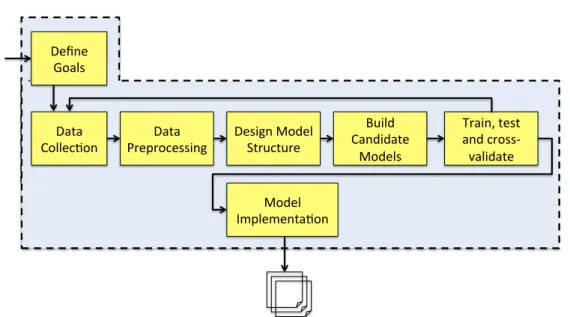
We advocate for achieving proactive self-adaptation by integrating predictive analysis into two phases of the software process. At design time, we propose a predictive modeling process, which includes the following activities: define goals, collect data, select model structure, prepare data, build candidate predictive models, training, testing and cross-validation of the candidate models and selection of the “best” models based on a measure of model goodness. At runtime, we consume the predictions from the selected predictive models using the running system actual data. Depending on the input data and the time allowed for learning algorithms, we argue that the software system can foresee future possible input variables of the system and adapt proactively in order to accomplish middle and long term goals and requirements.

The proposal has been validated with a case study from the environmental monitoring do-main. Validation through simulation has been done based on real data extracted from public environmental organizations. The answers to several research questions demonstrated the feasi-bility of our approach to guide the proactive adaptation of pervasive systems at runtime.

7

Résumé en Français

0.1

Introduction

Au cours des dernières années, il ya un intérêt croissant pour les systèmes logiciels capables de faire face à la dynamique des environnements en constante évolution. Actuellement, les systèmes auto-adaptatifs sont nécessaires pour l’adaptation dynamique à des situations nouvelles en maxi-misant performances et disponibilité [97]. Les systèmes ubiquitaires et pervasifs fonctionnent dans des environnements complexes et hétérogènes et utilisent des dispositifs à ressources li-mitées où des événements peuvent compromettre la qualité du système [123]. En conséquence, il est souhaitable de s’appuyer sur des mécanismes d’adaptation du système en fonction des événements se produisant dans le contexte d’exécution.

En particulier, la communauté du génie logiciel pour les systèmes auto-adaptatif (Software Engineering for Self-Adaptive Systems - SEAMS) [27, 35] s’efforce d’atteindre un ensemble de propriétés d’autogestion dans les systèmes informatiques. Ces propriétés d’autogestion com-prennent les propriétés dites self-configuring, self-healing, self-optimizing et self-protecting [78]. Afin de parvenir à l’autogestion, le système logiciel met en œuvre un mécanisme de boucle de commande autonome nommé boucle MAPE-K [78]. La boucle MAPE-K est le paradigme de référence pour concevoir un logiciel auto-adaptatif dans le contexte de l’informatique autonome. Cet modèle se compose de capteurs et d’effecteurs ainsi que quatre activités clés : Monitor, Ana-lyze, Plan et Execute, complétées d’une base de connaissance appelée Knowledge, qui permet le passage des informations entre les autres activités [78].

L’étude de la littérature récente sur le sujet [109, 71] montre que l’adaptation dynamique est généralement effectuée de manière réactive, et que dans ce cas les systèmes logiciels ne sont pas en mesure d’anticiper des situations problématiques récurrentes. Dans certaines situations, cela pourrait conduire à des surcoûts inutiles ou des indisponibilités temporaires de ressources du système [30]. En revanche, une approche proactive n’est pas simplement agir en réponse à des événements de l’environnement, mais a un comportement déterminé par un but en prenant par anticipation des initiatives pour améliorer la performance du système ou la qualité de service.

0.2

Thèse

Dans cette thèse, nous proposons une approche proactive pour l’adaptation dynamique. Pour améliorer l’adaptation dynamique nous proposons d’intégrer une activité Predict entre les acti-vités Analyze et Plan de la boucle MAPE-K. Nous nous appuyons sur des idées et des techniques du domaine de l’analyse prédictive pour réaliser l’activité Predict en charge de prédire. Selon les données d’entrée et le temps accordé pour les algorithmes d’apprentissage, nous soutenons

8

qu’un système logiciel peut prévoir les futures valeurs d’entrée possibles du système et s’adapter de manière proactive afin d’atteindre les objectifs et les exigences du système à moyen et long terme.

Nous plaidons pour la réalisation de l’auto-adaptation proactive en intégrant l’analyse pré-dictive dans deux phases du processus logiciel. Au moment de la conception, nous proposons un processus de modélisation de prédiction, qui comprend les activités suivantes : définir des objec-tifs, recueillir des données, sélectionner la structure modèle, préparer les données, construire des modèles prédictifs candidats, configurer ces modèles par l’apprentissage, réaliser des essais et la validation croisée des modèles candidats, sélectionner le meilleur modèle en se fondant sur une mesure de de performances. À l’exécution, nous employons des modèles prédictifs sélectionnés en utilisant le système des données réelles de fonctionnement. Selon les données d’entrée et le temps imparti pour les algorithmes d’apprentissage, nous soutenons que le système logiciel peut prévoir les valeurs futures des variables d’entrée du système et permettre ainsi d’adapter de manière proactive afin d’atteindre les objectifs de moyen et long terme et exigences.

0.3

Scénario de Motivation

La proposition a été motivée et validée par une étude de cas portant sur la surveillance de l’envi-ronnement. Supposons qu’une forêt est équipée d’un réseau sans fil de capteurs et de nœuds de calcul (WSN), qui sont déployés géographiquement à des endroits stratégiques. Chaque nœud de calcul peut accueillir entre un et trois capteurs physiques (par exemple, les précipitations, l’humidité et température). Le but du système est de réguler de nouvelles reconfigurations (par exemple augmenter ou diminuer le débit de transmission de capteurs) selon les prévisions des futurs paramètres de valeur pour améliorer l’efficacité et d’étendre la durée de vie du système. La figure 1 illustre notre scénario concret. Les capteurs communiquent avec le système de ges-tion du réseau de capteurs (WSN) pour obtenir des configurages-tions optimales en foncges-tion des conditions actuelles.

0.4

Contributions

Les contributions principales de cette thèse sont les suivantes :

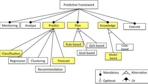
C1 : Extension du cadre d’architecture de référence Monitor-Analyze-Plan-Execute et Know-ledge(MAPE-K) [78]. Nous proposons de renforcer l’adaptation dynamique en intégrant une phase Predict entre les phases Analyze et Plan.

C2 : Nous proposons une technique pour la mise en œuvre du processus de modélisation pré-dictive, selon les sept étapes suivantes : (1) définir des objectifs, (2) recueillir des données, (3) définir la structure du modèle, (4) traiter les données, (5) construire les modèles can-didats, (6) réaliser l’apprentissage, tester et valider les modèles, et (7) mettre en œuvre les modèles.

C3 : Démonstration de notre approche avec un exemple concret tiré du domaine des Cyber-Physical Systems (CPS)(dans notre cas, surveillance de l’environnement).

9

FIGURE1 – L’application de surveillance de l’environnement réseau de capteurs sans fil [98])

0.5

Mise en Œuvre et Validation

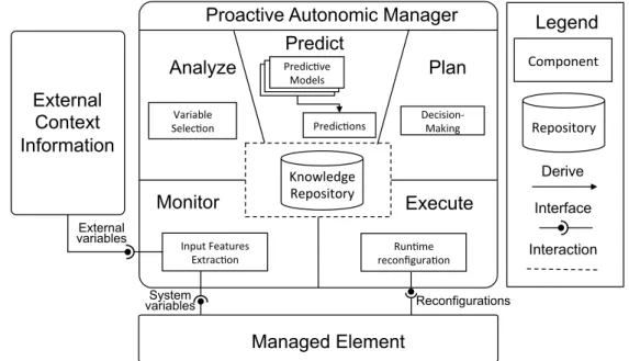
Les différentes contributions de cette thèse ont été concrétisées et intégrées dans une architecture de référence de type MAPE-K [78] (voir la figure 2). Les composants concrétisant notre cadre prédictif peuvent être divisés en deux phases : la phase de conception et la phase d’exécution.

La phase de conception inclut la configuration hors ligne de l’approche. Dans cette phase, nous effectuons des activités liées au processus de modélisation prédictive. Cela comprend des activités telles que la collecte de données, le prétraitement des données, de construire les mo-dèles candidats, réaliser l’apprentissage, tester et évaluer des momo-dèles prédictifs fondés sur des observations de données passées.

La phase d’exécution implique les activités mentionnées dans la boucle MAPE-K, en com-mençant par la surveillance et l’analyse de l’état actuel du système en ligne. Pendant la phase en ligne, nous évaluons les modèles prédictifs définis au moment de la conception. Cette évalua-tion est effectuée de deux manières : comparaison des stratégies réactives contre des stratégies d’adaptation proactives. Ensuite, en prenant en considération les résultats de l’évaluation nous procédons à la prise de décision de reconfiguration. La phase en ligne porte alors sur les nou-velles ré-configurations.

Nous avons évalué notre approche avec le système de surveillance de l’environnement senté comme scénario de motivation. À cette fin, nous avons employé un logiciel d’analyse pré-dictive open source (KNIME), des standard de modélisation prépré-dictive (p. ex. Prepré-dictive Mode-ling Markup Language (PMML)) et des API et outils deMachine learning APIs (e.g., R, octave, Weka).

Tout d’abord, nous avons modélisé une wireless sensor network (WSN) pour la détec-tion précoce des départs de feu, où nous combinons des données de température fournies par

10 Run$me' reconfigura$on' Input'Features' Extrac$on' Variable' Selec$on' Predic$ve' Models' Predic$ve' Models' Predic$ve' Models' Predic$ons' Decision? Making' ���������������� ���������������������������� Knowledge' Repository' �������� �������� ����� �������� �������� ���������� ��������� ������������ Component' ������� Repository' ������� ���������� ������������ ����������������� ������� ���������� ���������� ����������

FIGURE2 – Extension de le boucle MAPE-K

le National Climatic Data Center (NCDC) et des rapports d’incendie de Moderate Resolution spectroradiomètre imageur(MODIS). Nous avons évalué plusieurs modèles de classification et prédit la probabilité d’incendie pour les prochaine N heures. Les résultats confirment que notre approche proactive surpasse un système réactif typique dans les scénarios avec comportement saisonnier.

0.6

Organisation de la thèse

La thèse comprend six chapitres, organisés comme suit : • Chapitre 1 : Introduit le sujet de cette thèse.

• Chapitre 2 : Décrit le contexte et les fondations de l’analyse prédictive et des systèmes logiciels autonomes, pour comprendre les sujets liés à cette thèse.

• Chapitre 3 : Présente l’état de l’art de l’auto-adaptation proactive dans trois domaine dif-férents : génie logiciel, intelligence artificielle et théorie et ingénierie du contrôle.

• Chapitre 4 : Présente en détail l’approche que nous proposons et son architecture MAP2 E-K. En outre, nous détaillons la phase de conception et la phase d’exécution de notre ap-proche.

• Chapitre 5 : Décrit les détails de mise en œuvre et l’évaluation du notre approche en comparant les stratégies réactives textit vs. proactives.

11

Contents

0.5 Mise en Œuvre et Validation . . . 9

0.6 Organisation de la thèse . . . 10 Contents 11 1 Introduction 15 1.1 Motivation . . . 16 1.2 Research Questions . . . 17 1.3 Research Objectives . . . 17 1.4 Contributions . . . 18 1.5 Evaluation . . . 18 1.6 Organization . . . 19 2 Background 21 2.1 Motivation Scenario . . . 21

2.1.1 Benefits of Proactive Adaptation . . . 23

2.1.2 Engineering and Adaptation Challenges . . . 23

2.2 Predictive Analysis . . . 24

2.2.1 Data is the New Gold . . . 25

2.2.2 Prediction Offers Real Value . . . 26

2.2.3 Machine-Learning . . . 30

2.2.4 Ensemble of Predictive Models . . . 31

2.2.5 Supporting Decision-Making . . . 33

2.3 Autonomic Computing . . . 33

2.3.1 The Self-* Properties . . . 34

2.3.2 The Autonomic Control Loop . . . 35

12 CONTENTS

3 State of the Art 39

3.1 Taxonomy of Self-Adaptive Systems . . . 39

3.1.1 Change Dimension . . . 41 3.1.2 Temporal Dimension . . . 42 3.1.3 Control Mechanisms . . . 43 3.1.4 Realization Issues . . . 45 3.2 Related Work . . . 45 3.2.1 Software Engineering . . . 46 3.2.2 Artificial Intelligence . . . 53 3.2.3 Control Theory/Engineering . . . 57 3.3 Synthesis . . . 60

4 Achieving Proactivity Based on Predictive Analysis 63 4.1 Overview of the Approach . . . 63

4.1.1 The Design Phase: The Predictive Modeling Process . . . 64

4.1.2 Integration Points in the Runtime Phase . . . 70

4.1.3 Application Scenarios . . . 74

4.2 Implementation of the Approach . . . 77

4.2.1 Predict Module . . . 78

4.2.2 Knowledge Module . . . 80

4.3 Summary of the Approach . . . 84

5 Implementation and Evaluation 87 5.1 Requirements of the Forest Monitoring Scenario . . . 87

5.2 Design Phase of the Approach . . . 87

5.2.1 Data Collection . . . 89

5.2.2 Data Processing . . . 90

5.2.3 Building Predictive Models . . . 92

5.2.4 Training and Cross-Validation of Predictive Models . . . 92

5.3 Runtime Phase of the Approach . . . 94

5.3.1 On-line Monitoring . . . 95

5.3.2 Variable Selection . . . 99

5.3.3 Decision-making and Deploying Reconfigurations . . . 101

5.4 Empirical Evaluation . . . 102

5.4.1 A Brief Introduction to the Goal/Question/Metric (GQM) Paradigm . . 102

5.4.2 Empirical Evaluation of Proactive vs. Reactive Strategies . . . 103

5.4.3 Evaluation in Terms of Number of Reconfigurations . . . 107

5.4.4 Evaluation in Terms of System Lifetime . . . 107

5.4.5 Evaluation in Terms of Late Fire Report . . . 109

5.5 Discussion . . . 110

CONTENTS 13

6 Conclusions and Perspectives 113

6.1 Conclusions . . . 113

6.2 Lessons Learned . . . 115

6.3 Perspectives . . . 116

6.3.1 Improving our approach . . . 116

6.3.2 Other possible application scenarios . . . 117

6.4 Publications and Dissemination Activities . . . 119

6.4.1 Projects . . . 120

Appendix 121 A Implementation Details 121 A.1 Time Series Analysis Background . . . 121

A.2 MODIS Active Fire Detections for CONUS (2010) . . . 122

A.3 ISH/ISD Weather Stations in MS, USA . . . 123

A.4 PMML: Predictive Model Markup Language . . . 124

A.5 Fit best ARIMA model to univariate time series . . . 128

List of Figures 131

List of Tables 133

Listings 135

Bibliography 137

15

Chapter 1

Introduction

In recent years, the expansion of computing infrastructure has caused software systems to be ubiquitous. Currently, computing environments blend into the background of our lives, basi-cally everywhere and anywhere [123]. This pervasive characteristic has drastibasi-cally increased the dynamicity and complexity of software systems. Usually the burden of managing such hetero-geneous computing environments (e.g., devices, applications and resources) falls on engineers, which must manually redesign applications and adjust their settings according to available re-sources. Today, systems are required to cope with variable resources, system errors and failures, and changing users priorities, while maintaining the goals and properties envisioned by the en-gineers and expected by the final users [97].

Since its early beginnings, the software engineering community has envisioned the devel-opment of flexible software systems in which modules can be changed on the fly [44]. More recently, this vision has been extended to consider software systems that are able to modify their own behavior in response to changes in their operating conditions and execution environment in which they are deployed [70]. This concept is widely known as self-adaptation and it has been a topic of study in various domain areas, including autonomic computing, robotics, control systems, programming languages, software architecture, fault-tolerant computing, biological computing and artificial intelligence [27, 35, 71].

In particular, the Software Engineering for Self-Adaptive Systems (SEAMS)1 _community

[27, 35] has been working towards achieving a set of self-management properties in software systems. These self-management properties include self-configuring, self-healing, self-optimizing and self-protecting [78]. In order to achieve self-management, the software system implements an autonomic control loop mechanism known as the MAPE-K loop [78]. The MAPE-K loop is the de facto paradigm to design self-adaptive software in the context of autonomic computing. This reference model consists of sensors and effectors as well as four key activities: Monitor, Analyze, Plan and Execute functions, with the addition of a shared Knowledge base that enables the passing of information between the other components [78].

Traditionally, the MAPE-K loop is a runtime model where the Monitor activity includes reading from sensors or probes that collect data from the managed system and environment. This information reflects the system’s current state and its context environment. The Analyze

16 CHAPTER 1. INTRODUCTION tivity involves organizing the data, which is then cleaned, filtered, pruned to portray an accurate model of the current state of the system. Subsequently, the Plan activity involves building the execution plans to produce a series of adaptations to be effected on the managed system. Finally, the Execute activity involves carrying out the changes to the managed elements through the ef-fectors. The propagated adaptations can be coarse-grained, for example enabling or removing functionality, or fine-grained for instance changing configuration parameters.

In 2001, P. Horn presented in [70] IBM’s perspective on the state of information technology and he coined the term Autonomic Computing. The author explained in an illustrative way the analogy of the autonomic nervous system of the human body compared to an autonomous software system. Adopting the same analogy, we can consider the human body has two main “reasoning” capabilities: “reflex” and “thinking”. Reactive techniques can be seen as a kind of reflex, since they involve a short term response to a particular stimulus. When the system is in a critical context, these adaptations can quickly reconfigure the system into an acceptable configuration. On the other hand, proactive techniques based on predictions resembles more the definition of “thinking”, because they involve learning mechanisms based on historical data that can analyze middle and long term goals.

In this thesis we propose to enhance dynamic adaptation by integrating a Predict activity between the Analyze and Plan activities of the MAPE-K loop. We leverage ideas and techniques from the area of predictive analysis [126] to operationalize the Predict activity. Depending on the input data and the time allowed to the learning algorithms, we argue that a software system can foresee future possible input variables of the system and adapt proactively in order to accomplish middle or long term goals and requirements.

1.1

Motivation

During the last couple of years there is a growing interest into self-adaptive systems [27, 35]. Recent literature surveys [37, 71, 109] present that most of the existing self-adaptive systems have a reactive nature. A reactive adaptation strategy is triggered when a problem occurs and then the system addresses it. This capability of reactiveness is not generally a disadvantage. However, for some specific domains (e.g., environmental monitoring, safety critical systems), it is required to have proactiveness in order to decrease the aftereffects of changes and to block change propagation. Accordingly, S. W. Cheng et al. [30] demonstrate that a reactive strategy of adaptation might optimize instantaneous utility. However, it may often be suboptimal over a long period of time when compared with a predictive strategy. This means there is a great demand for proactive decision-making strategies.

A common scenario where the proactive strategy has the potential to outperform the reac-tive strategy regards applications that experiment cyclical behaviors. For instance, a personal laptop running on battery has several scheduled background tasks (e.g., backup, virus scan, up-dates) that can run periodically (e.g., daily, weekly). Often the execution of these administrative tasks cannot be interrupted or suspended once they have started, but the time and length of the execution is known beforehand. The resource utilization imposed by such tasks has a known behavior and it can certainly be predictable. Failure to recognize this behavior and not estimate its resource consumption in advance may lead to the system’s halt in the middle of a critical

CHAPTER 1. INTRODUCTION 17

update.

Although certainly not a new technology, predictive analysis ( a.k.a. predictive analytics) is a statistical or data analysis solution consisting of algorithms and techniques that can be used on both structured and unstructured data to determine possible outcomes [126]. Predictive analytics in software engineering has been widely used and has many application fields, thereby becoming a mainstream technology. The application fields include medical diagnostics, fraud detection, recommendation systems, and social networks. It is also being used for bank companies to perform credit risk assessment [112].

In general, predictive analysis can be used to solve many kinds of problem. In this thesis we argue that it can be applied to solve self-optimizing, self-protecting and self-configuring prob-lems. For instance, a software system self-optimizes its use of resources when it may decide to initiate a change to the system proactively, as opposed to adapting reactively, in an attempt to improve performance or quality of service [71]. In contrast to that, from our own perspective, the implementation of the self-healing property can be seen as a reactive adaptation strategy due to the fact that by its definition it aims at solving a problem that has previously occured.

1.2

Research Questions

The overall goal of this thesis can be formulated as follows:

How should predictive analysis be performed when the main purpose of prediction is to support proactive self-adaptation in pervasive systems?

Two important points here are purpose and context. The purpose of our study is predictive modeling as means to support proactive self-adaptation. The context is self-adaptive systems that implement the autonomic control loop. More in particular, we deal with pervasive sys-tems deployed in heterogeneous and dynamic environments. In order to narrow the aspects of integrating predictive modeling with self-adaptive systems that are investigated, three partial research questions are formulated:

RQ1: How do several measurements observed in the monitoring component correlate over a certain period of time?

RQ2: How to build a machine-learning predictive model based on the temporal behavior of many measurements correlated to externally known facts?

RQ3: What measurements might indicate the cause of some event, for example, do similar patterns of measurements preceded events that lead to a critical situation such as a failure, and how to diagnosis this causal relationship?

1.3

Research Objectives

The major goal of this thesis is to propose a predictive analysis based approach using ma-chine learning techniques and integrate it into the autonomic control loop in order to

en-18 CHAPTER 1. INTRODUCTION able proactive adaptation in self-adaptive systems. Therefore, this thesis targets the following objectives:

RO1: Explore proactive adaptation approaches that leverages on existing context and environ-ment streams of data in order to anticipate erroneous behavior of the system by predicting conflicting situations.

RO2: Study the activeness (e.g., reactive vs. proactive) of self-adaptive systems, analyze the potentials and limitations of system’s parameters predictability (e.g., prediction horizon, prediction granularity), and investigate solutions to deal with parameter’s future value uncertainty (e.g., prediction confidence level).

RO3: Develop a methodological framework of predictive modeling using machine learning techniques to enhance the effectiveness of proactive adaptation in self-adaptive software systems.

1.4

Contributions

The study and analysis of the aforementioned research objectives has generated the following contributions:

C1: Extension of the Monitor-Analyze-Plan-Execute and Knowledge (MAPE-K) reference ar-chitecture [78]. We propose to enhance dynamic adaptation by integrating a Predict phase between the Analyze and Plan phases.

C2: We propose a stepwise technique for the operationalization of the predictive modeling pro-cess divided in seven steps, namely: (1) define goals, (2) collect data, (3) define model structure, (4) data processing, (5) build candidate models, (6) train, test and validate mod-els, and (7) models implementation.

C3: The demonstration of our approach with a concrete example taken from the Cyber-Physical Systems (CPS) domain (e.g., environmental monitoring). This implementation is de-scribed in more detail in Chapter 5.

1.5

Evaluation

We evaluated our approach in the environmental monitoring system presented on the motivation scenario. For this purpose, we implemented the proposed approach using an open source predic-tive analysis framework (i.e. KNIME), predicpredic-tive modeling standards (e.g., Predicpredic-tive Modeling Markup Language (PMML)) and machine learning libraries/tools (e.g., R, Octave, Weka).

Firstly, we modeled a wireless sensor network (WSN) for early detection of fire conditions, where we combined hourly temperature readings provided by National Climatic Data Center (NCDC) with fire reports from Moderate Resolution Imaging Spectroradiometer (MODIS) and simulated the behavior of multiple systems. We evaluated several classification models and predicted the fire potential value for the next N hours. The results confirmed that our proactive approach outperforms a typical reactive system in scenarios with seasonal behavior [98].

CHAPTER 1. INTRODUCTION 19

1.6

Organization

The rest of this thesis is organized as follows:

• Chapter 2 describes the background and the foundations in predictive analytics and auto-nomic computing to understand the subjects related to this dissertation.

• Chapter 3 overviews the state of the art in proactive self-adaptation approaches coming from three different domain areas: software engineering, artificial intelligence and control theory/engineering.

• Chapter 4 describes our proposed MAP2E-K loop in detail. Additionally, we elaborate the design phase and runtime phase of our approach. These phases include the following activities: data collection, prepare data, build predictive models, training, testings and cross-validation of models, implementation of predictive models and implementation of the models.

• Chapter 5 describes the implementation details and the evaluation of the proposed proac-tive framework comparing the reacproac-tive vs. proacproac-tive strategies.

21

Chapter 2

Background

This chapter presents the foundations to understand the subjects related to this thesis. Firstly, in Section 2.1 we present a motivation scenario extracted from the environmental monitoring domain to illustrate the research problem we are tackling on. Secondly, in Section 2.2 we present Predictive Analysis [126], which is one of the building blocks for proactive self-adaptation. Thirdly, in Section 2.3 we present in details the area of Autonomic Computing [70], which is another domain area that enables our research approach. Finally, in Section 2.4 we discuss some similarities and potential conflicting issues in the previously described disciplines and give some conclusions.

2.1

Motivation Scenario

In this section we describe our motivation scenario that is at the heart of the problem we are focusing on. Let us assume that a forest is equipped with a wireless sensor network (WSN), where sensor-nodes are deployed geographically at strategic locations. Each sensor-node can host between one and three physical sensors (e.g., precipitation, humidity and temperature).

The goal of the system is to regulate new reconfigurations (e.g., increase or decrease sensor’s transmission rate) according to predictions of future value parameters to improve the effectiveness and extend the life span of the system. Figure 2.1 illustrates our motivation scenario. Sensors communicate with the environment wireless sensor network (WSN) manage-ment system to obtain optimal configurations according to current conditions.

Each sensor node component is functioning at a standard sampling rate. However, the trans-mission of data can be controlled using three different levels of transtrans-mission rate: LOW (e.g., 1 transmission every 24 hours), MEDIUM (e.g., 1 transmission every 8 hours) and HIGH (e.g., 1 transmission every hour). Sensor nodes are equipped with 6lowPan radio for inter-node com-munication. Data-collector nodes are in charge of receiving raw data from the sensor-nodes and perform as gateway of the system.

The environmental WSN monitoring system has a global entity, which has access to all avail-able information from sensors and maintains a global model of the current state of the system. In this context, the environmental manager has access to weather forecast and historical informa-tion of actual fires in similar locainforma-tions. Combining both data sources, we can relate individual

22 CHAPTER 2. BACKGROUND

Figure 2.1 – Environmental monitoring wireless sensor network [98])

fires to weather conditions in space and time. The environmental WSN can be considered as a cloud-based dedicated service that decides the reconfiguration of each sensor-node, taking into account the following relevant parameters: (i) position, (ii) battery life and (iii) current environ-mental condition expressed as a cost function of precipitation, temperature and humidity.

A stochastic model predicts the forest behavior based on historical data. The model’s accu-racy is a function of the transmission rate, number and distribution of sensor-nodes contributing raw data through the data-collectors. Therefore, there is an implicit need to evolve the initial configuration over time because of system constrains or environmental changes (e.g., batteries are running low, or because a seasonal drought requires a more frequent and accurate transmis-sion of current conditions).

To sum up, the main requirements of the environment monitoring motivation scenario are: 1. The system should provide feedback on potential fire risks to its users (e.g., environmental

guards, fire department) allowing them to act proactively and anticipate and avoid possible critical situations.

2. The system should support the coordinated reconfiguration of sensor nodes, in order to avoid service failure due to battery exhaustion, with the goal of extending the life time of the system as much as possible.

The approach we propose assumes that the following information technologies are available: 1. The forest is equipped with a wireless sensor network, where each node has several sens-ing capabilities (e.g., temperature, humidity, smoke). Sensor nodes can communicate among themselves (i.e. intra-node communication) and with external data collector de-vices (i.e., extra node communication) to transmit the raw data.

CHAPTER 2. BACKGROUND 23

2. Nodes can be reconfigured via wireless. Reconfigurations represent changes by increasing or decreasing the transmitting frequency (e.g., every 1 hr, 4 hrs, 8 hr). Other kind of adap-tation may involves enabling or disabling sensor capabilities (e.g., enabling temperature) or changing the sleeping and wake up cycle in the sensor nodes.

2.1.1 Benefits of Proactive Adaptation

Proactive adaptation offers the benefit of anticipating events in order to optimize system behavior with respect to its changing environment. By analyzing the limitations of the reactive strategy, we have identified three potential benefits under which the proactive approach is likely to be better than the reactive strategy:

1. Avoiding unnecessary adaptation: This happens when the conditions that trigger an adap-tation may be more short-lived than the duration for propagating the adapadap-tation changes. 2. Managing allocation of exhaustible resources: by managing allocation of perishable

re-sources (e.g., battery) with proactive adaptation enable us to make provision for future time when the resource is scarce.

3. Proactivity in front of seasonal behavior: proactive adaptation in front of seasonal behav-ior requires detecting seasonal patterns, which can be provided by predictors like time-series analysis.

2.1.2 Engineering and Adaptation Challenges

Engineering self-adaptive system deployed in dynamic and ever-changing environments poses both engineering and adaptation challenges. These challenges can be briefly described in terms of the following quality of services (QoS) properties:

Proactivity: Proactivity captures the anticipatory aspect in self-adaptive system. It can be

broadly defined as the ability of the system to anticipate and predict when a change or problem is going to occur, and to take action about it [109]. On the contrary, in a reac-tive mode the system responds when a change or problem has already happened. When dealing with dynamically adaptive systems, as in our previously described motivation sce-nario, reactiveness has some limitations: (i) information used for decision making does not extend into the future, and (ii) the planning horizon of the strategy is short-lived and does not consider the effect of current decisions on future utility [30].

Predictability: Predictability can be described in two ways: predictability associated with the

environment, which is concerned with whether the source of change can be predicted ahead of time, and predictability associated with the running system, which deals with whether the consequences of self-adaptation can be predictable both in value and time [4]. In the context of this thesis we are concerned with predictability associated to the envi-ronment and the different techniques need it depending on the degree of anticipation.

24 CHAPTER 2. BACKGROUND

Reliability: Reliability can be broadly defined as the probability of successfully accomplishing

an assigned task when it is required [46]. In particular, the meaning of success is domain dependent, for instance, that the execution of the task satisfies convenient properties (e.g., it has been completed without exceptions, within an acceptable timeout, occupying less than a certain amount of memory, etc).

Attaining the previously described QoS properties poses a great challenge and illustrates the opportunity of improvement in the existing adaptation approaches. Currently, there is an over-abundance of public data (e.g., sensors, mobiles, pervasive systems). Thus, there is great demand for solutions to make sense of this data, particularly using predictive mechanisms regarding the specific domain and its operational environment. In the following section we explore in detail the enablers of proactivity, predictability and reliability in the context of self-adaptive systems.

2.2

Predictive Analysis

This section presents predictive analysis as an enabler of our proactive self-adaptation approach. Predictive analysis (PA) encompasses a variety of statistical techniques ranging from modeling, machine learning, and data mining techniques that analyze current and historical facts to make predictions about future, or otherwise unknown, events [95].

Currently, there is an explosion of data being collected everywhere around ever increasing and ubiquitous monitoring processes. Data continues to grow and hardware is struggling to keep up, both in processing power and large volume data repositories [126]. Data can be broadly categorized as either structured or unstructured. Structured data has well-defined and delimited fields, and this is the usual type of data used in statistical modeling. Unstructured data includes time series, free text, speech, sound, pictures and video. Statistical modeling can also be divided into two broad categories: search and prediction. For search problems we try to identify cate-gories of data and then match search requests with the appropriate data records. In prediction problems we try to estimate a functional relationship, so we can provide an output to a set of inputs. These prediction statistical models are in general the types of modeling problems that are considered in this thesis.

E. Siegel, in his book Predictive Analytics: The power to predict who will click, buy, lie or die[112] presented 147 examples of different application domains for predictive analytics. Applications can be found in a wide range of different domains including: stock prices, risk, accidents, sales, donations, clicks, health problems, hospital admissions, fraud detection, tax evasion, crime, malfunctions, oil flow, electricity outages, opinions, lies, grades, dropouts, ro-mance, pregnancy, divorce, jobs, quitting, wins, votes, and much more.

The predictive analysis process is generally divided in two parts: off-line and on-line. The off-line phase involves collecting the data from the environment and applying the machine-learning techniques to the datasets to build predictive models. The on-line phase include the activities of characterization of an individual, next the individual is evaluated with predictive models in order to generate the results that will drive the decision-making process. Figure 2.2 illustrates the general predictive analysis process and the relationships between its main compo-nents.

CHAPTER 2. BACKGROUND 25 ��������� �������� ����� ���������_{���������} ���������������� ����������������� � ����������� ������ � ������������ ������ �

Figure 2.2 – General overview of the predictive analysis process (based on [112]) Namely, the basic elements that make feasible the predictive analysis process are: data, predictions, machine-learning, ensemble of models and the action of decision-making [112, 126]. The following subsections explain in more detail each element and their relationships in the predictive analysis process.

2.2.1 Data is the New Gold

Following the agricultural and industrial revolutions from previous centuries, in the last decades we have experienced the information revolution [103]. Forbes, the American business magazine stated that we are entering a new era, the era of data where data is the new gold1_{. Several other}

authors have coined data as “the new oil” or “data is the new currency of the digital world” [103]. Day by day, each on-line and off-line bank transaction is recorded, websites visited, movies watched, links clicked, friends called, opinions posted, dental procedures endured, sports games won, traffic cameras passed and flights taken. Countless sensors are deployed daily. Mobile de-vices, drones, robots, and shipping containers record movement, interactions, inventory counts, and radiation levels, just to mention a few devices that generate and consume data. Now imag-ine all those deployed devices interconnected at an unprecedented scale and pace, this is what is known as the Internet of Things (IoT), a term first coined by Kevin Ashton in 1999 in the con-text of supply chain management [7]. The next revolution will be the interconnection between objects to create a smart environment. Only in 2011 did the number of interconnected devices on the planet overtake the actual number of people. Currently there are 9 billions interconnected devices and it is expected to reach 24 billions devices by 2020 [62].

Further more, free public data is overflowing and waiting at our fingertips. Following the open data movement, often embracing a not-for-profit organization, many data sets are available on-line from different fields like biodiversity, business, cartography, chemistry, genomics, and

26 CHAPTER 2. BACKGROUND medicine. For example KDnuggets2 _{is one of the top resource since 1997 for data mining and}

analytics. Another example is the United States official website Data.gov, whose goal is “to increase public access to high value, machine readable datasets generated by the Government of USA.” Data.gov3 _{contains over 390,000 data sets, including data about marine casualties,}

pollution, active mines, earthquakes, and commercial flights [103].

Big data is defined as data too large and complex to capture, process and analyze using current computer infrastructure. It is now popularly characterized by five V’s (initially it was described as having three, but two have since then been added to emphasize the need for data authenticity and business value) [63]:

• Volume: data measurements in tera (1012) are now the norm, or even peta (1015_{), and is}

rapidly heading towards exa (1018_);

• Velocity: data production occurs at very high rates, and because of this sheer volume some applications require near real-time data processing to determine whether to store a piece of data;

• Variety: data is heterogeneous and can be highly structured, semi-structured, or totally unstructured;

• Veracity: due to intermediary processing, diversity among data sources and in data evo-lution raises concerns about security, privacy, trust, and accountability, creating a need to verify secure data provenance; and

• Value: through predictive models that answer what-if queries, analysis of this data can yield counterintuitive in sights and actionable intelligence.

With such an overflow of free public data, there is a need for new mechanisms to analyze, process, and take advantage of its great potential. Thus, the goal is to apply predictive analysis techniques to process this abundance of public data. This involves a variety of statistical tech-niques such as modeling, machine learning, and data mining that analyze current and historical facts in order to make predictions about future or unknown events [95]. New data repository structures have evolved, for example the MapReduce/Hadoop4 _{paradigm. Cloud data storage}

and computing is growing, particularly in problems that can be parallelized using distributed processing [63].

2.2.2 Prediction Offers Real Value

J. A. Paulos, professor of mathematics at Temple University in Philadelphia defined “Predic-tion is a very difficult task and uncertainty is the only certainty there is. Knowing how to live with insecurity is the only security”. Thus, uncertainty is the reason why accurate prediction is generally not possible. In other words, predicting is better than pure guessing, even if is not

2_{http://www.kdnuggets.com/datasets/index.html} 3_{http://www.data.gov/}

CHAPTER 2. BACKGROUND 27

100 percent accurate, predictions deliver real value. A vague view of what is coming outper-forms complete darkness [112]. Therefore analyzing errors is critical. Learning how to replicate past successes by examining only the positive cases does not work and induces over-fitting to the training data [89]. Thus, negative examples are our friends and should be taken into account. From Figure 2.2 that illustrates the predictive analysis process we see that before using a predictive model we have to build it using machine learning techniques. By definition a predic-tive modelis a mechanisms that predicts a behavior of a system. It takes characteristics of the system as input (e.g. internal, external), and provides a predictive score as output. The higher the score, the more likely it is that the system will exhibit the predicted behavior [112].

From the predictive analysis process we can clearly identify two phases. In the off-line phase data must be collected and processed. This means identifying the predictor variables, which are the parameters that better describe the behavior of the system. This part also involves cleaning the data, which can be done by re-dimensional analysis and removing out-layers from the training dataset. Alternatively, surrogate variables can be used to handle missing values of predictor variables. Next, the machine learning algorithms crunches the data to build the predictive model.

In general, the statistical modeling approaches can be categorized in many ways [15], for instance: (1) classification, i.e. predicting the outcome from a set of finite possible values, (2) regression, i.e. predicting a numerical value, (3) clustering or segmentation, i.e. summa-rizing data and identifying groups of similar data points, (4) association analysis, i.e. finding relationships between attributes, and (5) deviation analysis, i.e. finding exceptions in major trends or structures. Other authors, such as [126], categorize the prediction approaches from a different perspective: (1) linear modeling and regression, (2) non-linear modeling, and (3) time series analysis.

In our case, we focused on classification and regression methods in the scope of time series analysis. Classification, because we focused on finding a model that, when applied on a certain time series (e.g. hourly temperature readings), is able to classify current weather conditions as having significant fire potential or not. Regression models are applied in the forecasting scope to make precise predictions for the next N hours in the time series.

Linear Modeling and Regression

The most common data modeling methods are regressions, both linear and logistic. According to [126], it is likely that 90% or more of real world applications of data mining end up with a relatively simple regression as the final model, typically after very careful data preparation, encoding, and creation of variables.

In statistics, linear regression is an approach for modeling the relationship between a scalar dependent variable y and one or more explanatory (or independent) variable denoted X. The case of one explanatory variable is called simple linear regression, whereas for more than one explanatory variable the process is called multiple linear regression.

There are several reasons why regressions are so commonly used. First, they are generally straightforward both to understand and compute. The mean square error (MSE) objective func-tion has a closed-form linear solufunc-tion obtained by differentiating the MSE with respect to the unknown parameter and setting the derivatives to zero.

28 CHAPTER 2. BACKGROUND Non-linear Modeling

Previously, we discussed many of the important and popular linear modeling techniques. Mov-ing one step towards complexity we can find the nonlinear models. These classes of models can be understood as fitting linear models into local segmented regions of the input space. Ad-ditionally, fully nonlinear models beyond local linear ones include: clustering, support vector machine (SVM), fuzzy systems, neural networks, and others. Formally defined, the goal of non-linear modeling is to find the best-fit hyper plane in the space of the input variables that gives the closest fit to the distribution of the output variable [126].

In particular, in Section 5.2.4 we choose from existing classification models and evalu-ate 8 non-linear models in the implementation of the motivation scenario. These models are: (1) Multi Layer Perceptron [107], (2) Fuzzy Rules [14], (3) Probabilistic Neural Network [16], (4) Logistic Regression [126], (5) Support Vector Machine [104], (6) Naive Bayes [126], (7) Ran-dom Forest [23], and (8) Functional Trees [55]. In general, the more nonlinear the modeling paradigm, the more powerful the model. However, at the same time, the easier it is to overfit. Time Series Analysis

One major distinction in modeling problems as time series analysis is that the next value of the series is highly related to the most recent values, with a time-decaying importance in this rela-tionship to previous values. Before looking more closely at the particular statistical methods, it is appropriate to mention that the concept of time series is not quite new. In fact its beginnings date back to mid-19th century, when ship’s captains and officers had long been in the habit of keep-ing detailed logbooks durkeep-ing their voyages (e.g., knots, latitude, longitude, wildlife, weather, etc.). Then they carried out analysis in the collected data that would enable them to recommend optimal shipping routes based on prevailing winds and currents [39].

Moreover, the time series forecasting problem has been studied during the last 25 years [34], developing a wide theoretical background. Nevertheless, looking back 10 years, the amount of data that was once collected in 10 minutes for some very active systems is now generated every second [39]. Thus, the current overabundance of data poses new challenges that need different tools and the development of new approaches.

The goal of modeling a problem in terms of time series analysis is to simplify it as much as possible regarding the time and frequency of generated data. R. H. Shumway and D. S. Stoffer categorized the time series analysis from two different approaches: time domain approach and frequency domain approach [111], see Figure 2.3.

The time domain approach is generally motivated by the presumption that correlation be-tween adjacent points in time is best explained in terms of a dependence of the current value on past values. Conversely, the frequency domain approach assumes the primary characteristics of interest in time series analyses relate to periodic or systematic sinusoidal variations found naturally in most data. The best way to analyzing many data sets is to use the two approaches in a complementary way.

• Time domain approach. The time domain approach focuses on modeling some future value of a time series as a parametric function of the current and past values. Formally, a

CHAPTER 2. BACKGROUND 29 ��������������������� ������ ��������� ������������������� ������������ ������ ���������������������� ������������� ����������������� ������������ ������������� ��������������� ��������������� ����������� �������� �������� ����������� �����������

Figure 2.3 – Time series approaches (based on [111])

time series X is a discrete function that represents real-valued measurements over time as represented in Formula 2.1.

X= {x1, x2...xn} : X = {xt : t ∈ T } : T = {t1,t2...tn} (2.1)

The n time points are equidistant, as in [90]. The elapsed time between two points in the time series is defined by a value and a time unit. For example, we may consider a time series as a sequence of random variables, x1; x2; x3; ... , where the random variable x1

denotes the value taken by the series at the first time point t1, the variable x2 denotes the

value for the second time period t2, x3 denotes the value for the third time period t3, and

so on. In general, a collection of random variables, xt, indexed by t is referred to as a

stochastic process. In this analysis, t will typically be discrete and vary over the integers t = 0; ± 1; ± 2; or some subset of the integers [111]. This time series generated from uncorrelated variables is used as a model for noise in engineering applications and it is called white noise [111].

If the stochastic behavior of all time series could be explained in terms of the white noise model, classical statistical methods would suffice. Two ways of introducing serial corre-lation and more smoothness into time series models are moving averages and autoregres-sions.

To smooth a time series we might substitute the white noise with a moving average by replacing every value by the average of its current value and its immediate neighbors in the past and future. For instance, the following Formula 2.2 represents a 3-point moving average.

vt=

1

30 CHAPTER 2. BACKGROUND Classical regression is often insufficient for explaining all of the interesting dynamics of a time series. Instead, the introduction of correlation as a phenomenon that may be generated through lagged linear relations leads to proposing the autoregressive (AR) and autoregressive moving average (ARMA)models. The popular Box and Jenkins [21] Au-toregressive integrated moving average (ARIMA)create models to handle time-correlated modeling and forecasting. The approach includes a provision for treating more than one input series through multivariate ARIMA or through transfer function modeling [22, 20]. • Frequency domain analysis. Seasonality can be identified and removed as follows. First we need to identify the natural periodicity of data. This can be done in a variety of ways, such as (a) through expert understanding of the dynamics, (b) through statis-tical analysis using different window lengths, or (c) through frequency analysis look-ing for the fundamental frequencies. Formally defined, a time series Xt with values

(xt−k, xt−k−1, ..., xt−2, xt−1) (where t is the current time) can be represented as the

addi-tion of four different time series:

Xt = Tt+ St+ Rt (2.3)

where Tt, St and Rt are the trend, seasonality and random components of the time series.

The trend Tt describes the long term movement of the time series. The seasonality

com-ponent St describes cyclic behaviors with a constant level in the long term, it consists of

patterns with fixed length influenced by seasonal factors (e.g., monthly, weekly, daily). Finally, the random component Rt is an irregular component to be described in terms of

random noise. Therefore, modeling Xtcan be described as the addition of its components.

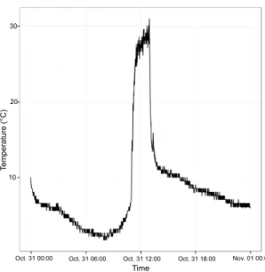
Figure 2.4 illustrates a time series decomposition analysis of a temperature variable over 30 days.

– The trend component can be described as a monotonically increasing or decreasing function, in most cases a linear function, that can be approximated using common regression techniques. It is possible to estimate the likelihood of a change in the trend component by analyzing the duration of historic trends.

– The seasonal component captures recurring patterns that are composed of at least on or more frequencies (e.g daily, weekly, monthly) patterns. These frequencies can be identified by using a Discrete Fourier Transformation (DFT) or by auto-correlation technique [111].

– The random component is an unpredictable overlay or various frequencies with dif-ferent amplitudes changing quickly due to random influences on the time series.

2.2.3 Machine-Learning

Machine Learning aims at finding patterns that appear not only in the data at hand, but in general, so that what is learned will hold true in new situations never yet encountered. By definition, “a computer program is said to learn from experience E with respect to some class of tasks T

CHAPTER 2. BACKGROUND 31 Temperature (deg C) 10 15 20 25 dat a − 6 − 2 0 2 4 6 seasonal 16 17 18 19 20 21 trend − 0. 3 − 0. 1 0. 1 remainder time (days) 0 5 10 15 20 25 30

Figure 2.4 – A time series decomposition analysis example

and performance measure P, if its performance at tasks in T, as measured by P, improves with experience E”, which has become the formal definition of Machine Learning [88]. Training data sets are use by machine learning algorithms to generate a predictive model. Testing data sets are used to evaluate the accuracy of the predictive models to the real data.

Table 2.1 shows a classification of datasets and a selection of candidate predictive models that can be applied to such datasets. Data sets can be organized by three characteristics: default task, data type and attribute type. This classification is based in the Machine Learning Repository (MLR)5_{from the University of California, School of Information and Computer Science [9].}

For each considered model there are myriads of variations proposed in the literature, and it would be a hopeless task to consider all existing varieties. Our strategy is therefore to consider the basic version of each model and categorize them by the purpose of their task, data type and attribute type. The rationale is that most users will more likely prefer to consider the basic form at least in their first attempt to understand its functionality.

2.2.4 Ensemble of Predictive Models

An ensemble of predictive models consists of a set of individually trained classifiers (e.g. neural networks, decision trees) whose results are combined to improve the prediction accuracy of a machine learning algorithm [126]. Previous research has shown that a collection of statistical classifiers, or ensembles, is often more accurate than a single classifier [95].

A random forest model is the typical example for predictive models ensemble used for clas-sification and regression problems. It operates by constructing a multitude of decision trees at training time and by outputting the class that is the mode of the classes output by individual trees [95]. The general abstraction is collecting models and having them vote. When joined as

32 CHAPTER 2. BACKGROUND

Property Types Definition

Default task

Classification Is a supervised problem where inputs are divided

into two or more classes known beforehand (e.g., Bayes, function, fuzzy, meta-classifiers, rule-based, trees, Support vector machines)

Regression Also a supervised problem, the outputs are

contin-uous rather than discrete (e.g. linear regression, lo-gistic regression, SVM)

Clustering A set of inputs is to be divided into groups. Unlike in classification, the groups are not known beforehand, making this typically an unsupervised task (e.g. centroid-based clustering, K-nearest, distribution-based clustering)

Recommendation Is an information filtering system that seek to predict the “rating” or “preference” that users would give to an item (e.g., collaborative filtering, content-based filtering, hybrid recommender).

Forecast Estimates a future event or trend as a result of

study and analysis of available pertinent data (e.g., Times series analysis, autoregressive moving aver-age (ARMA), autoregressive integrated moving av-erage (ARIMA), Holt-Winters (HW))

Data type

Univariate Considers only one factor, or predictor variable,

about the system under study

Multivariate Considers multiple factors or predictor variables at a time of the system under study

Sequential Considers sequence of data values, usually ordinal

or categorical data (e.g. months of the year, days of the week)

Time Series Considers a set of values of a quantity obtained at

successive times, often with equal intervals between them (e.g. hourly temperature readings)

Tex Considers text collections that belongs to a

vocabu-lary or specific language (e.g. used for spam filter-ing)

Attribute type

Categorical Considers qualitative attributes

Numerical Considers quantitative attributes

Mixed Support both qualitative and quantitative attributes

CHAPTER 2. BACKGROUND 33

ensembles, predictive models compensate for their limitations, so the ensemble as a whole is more likely to have higher accuracy rather than its individual predictive models.

Another example of model ensembles is boosting algorithms, which is an approach to ma-chine learning based on the idea of creating a highly accurate predictor by combining many weak and inaccurate learners. Some popular algorithms in this category are AdaBoost, LPBoost, To-talBoost, BrownBoost, MadaBoost, among others [110].

2.2.5 Supporting Decision-Making

Once the predictive model or the ensembles of predictive models is trained and tuned, the next step is to deploy it on-line. The key part is to integrate it with a decision-making mechanism. In a previous paper we integrated our prediction based proactive approach with a ruled-based mechanism to take decisions whether to adapt or not the software system [98].

Prediction does not offer a real value by itself unless it feeds a reasoning engine to support the decision-making process. Therefore, prediction implies action. Particularly, in the imple-mentation of our approach we observed that predictions offer three kinds of improvement when compared to existing reactive adaptation approaches:

1. Prediction prevents unnecessary self-adaptation: At times the conditions that triggers an adaptation may be more short-lived that the duration for propagating the adaptation changes, resulting in unnecessary adaptation that incur potential resource cost and service disruption [30].

2. Prediction to manage the allocation of exhaustible resources: In [93], the author proposed a taxonomy that classifies each computing resources into one of three categories: time-shared, space-shared and exhaustible. For instance, CPU and bandwidth are time-shared resources, while battery is an exhaustible resource. A proactive strategy offers the advan-tage to make provision of exhaustible resources (e.g., battery) for future time when the resource is scarce [98].

3. Proactivity in front of seasonal behavior: If a similar shift in system conditions occurs seasonally, this means once every period of time such as every day at 10 AM, the same pattern of adaptations would repeat every period. One workaround is to learn the seasonal pattern from historical data and predict adaptations on time [30].

2.3

Autonomic Computing

Autonomic Computingis the other enabler of our approach. Autonomic computing is an IBM´s initiative presented P. Horn [70] in 2001. It describes computing systems that are said to be self-managing. The term “autonomic” comes from a biology background and is inspired by the human body’s autonomic nervous system. Similarly, a self-adaptive system (SAS) modifies its own behavior in response to changes in its operating environment, which is anything observable by the software system, such as end-user inputs, external hardware devices and sensors, or pro-gram instrumentation [97]. The concepts of autonomic computing and self-adaptive systems are

34 CHAPTER 2. BACKGROUND strongly related and share similar goals, thus within the scope of this thesis both terms are used interchangeably.

Autonomic computing original goal is:

“To help to address complexity by using technology to manage technology. The term autonomic is derived from human biology. The autonomic nervous system monitors your heartbeat, checks your blood sugar levels and keeps your body tem-perature closer to 98.6◦_{F without any conscious effort on your part. In much the}

same way, self-managing autonomic capabilities anticipate and resolve problems with minimal human intervention. However, there is an important distinction be-tween autonomic activity in the human body and the autonomic activities in IT systems. Many of the decisions made by autonomic capabilities in the body are involuntary. In contrast, self-managing autonomic capabilities in software systems perform tasks that IT professionals choose to delegate to the technology according to policies [70].”

As mentioned earlier, Autonomic Computing (AC) and Self-adaptive System (SAS) share the same goal, which is to improve computing systems with a decreasing human involvement in the adaptation process. Many researchers use the terms self-adaptive, autonomic computing, and self-managing interchangeably [32, 37, 71]. Salehie and Tahvildari [109] describe a slightly dif-ferent point of view, where “the self-adaptive software domain is more limited, while autonomic computing has emerged in a broader context.” According to the authors [109] “self-adaptive software has less coverage and falls under the umbrella of autonomic computing.”

2.3.1 The Self-* Properties

Upon launching the AC initiative, IBM defined four general adaptivity properties that a system should have to be considered self-managing. These properties are also knowns as the self-* propertiesand include: self-configuring, self-healing, self-optimizing and self-protecting. These properties are described as follows.

Self-configuringis the capability of reconfiguring automatically and dynamically in response

to changes by installing, updating, integrating, and composing/decomposing software en-tities [109].

Self-optimizingis the capability to monitor and tune resources automatically to meet end-users

requirements or business needs [70]. An autonomic computing system optimizes its use of resources. It may decide to initiate a change to the system proactively, as opposed to a reactive behavior, in an attempt to improve performance or quality of service [71].

Self-healingis the capability of discovering, diagnosing and reacting to disruptions [78]. The

kinds of problems that are detected can be interpreted broadly: they can be as low-level as bit errors in a memory chip (hardware failure) or as high-level as an erroneous entry in a directory service. Fault tolerance is an important aspect of self-healing [71].