HAL Id: tel-01560566
https://tel.archives-ouvertes.fr/tel-01560566
Submitted on 11 Jul 2017HAL is a multi-disciplinary open access
archive for the deposit and dissemination of sci-entific research documents, whether they are pub-lished or not. The documents may come from teaching and research institutions in France or abroad, or from public or private research centers.
L’archive ouverte pluridisciplinaire HAL, est destinée au dépôt et à la diffusion de documents scientifiques de niveau recherche, publiés ou non, émanant des établissements d’enseignement et de recherche français ou étrangers, des laboratoires publics ou privés.
acides du Massif Central (France)
Arnaud Duranel
To cite this version:
Arnaud Duranel. Hydrologie et modélisation hydrologique des tourbières acides du Massif Central (France). Géographie. Université de Lyon, 2016. Français. �NNT : 2016LYSES012�. �tel-01560566�
THESE de DOCTORAT DE L’UNIVERSITE DE LYON
opérée au sein de
l’Université Jean Monnet
Ecole Doctorale N° 483
Sciences Sociales
Spécialité de doctorat : Géographie
Soutenue publiquement le 23/03/2016, par :
Arnaud DURANEL
Hydrologie et modélisation
hydrologique des tourbières acides du
Massif Central (France)
Devant le jury composé de :
Hervé PIÉGAY, Directeur de Recherche au CNRS, UMR CNRS 5600 EVS, Université de Lyon, Université Jean Moulin, Président
Luc AQUILINA, Professeur, Géosciences Rennes UMR CNRS 6118, Université de Rennes 1, Rapporteur
André-Jean FRANCEZ, Maître de Conférences-HDR, UMR ECOBIO 6553 – IFR CAREN, Université de Rennes 1, Rapporteur
Fatima LAGGOUN-DÉFARGE, Directrice de Recherche au CNRS, Observatoire des Sciences de l’Univers en région Centre, Université d’Orléans, Examinatrice
Didier GRAILLOT, Directeur de Recherche, UMR 5600 CNRS, École Nationale des Mines de Saint-Étienne, Examinateur
Robert WYNS, Géologue, Bureau de Recherches Géologiques et Minières, Orléans, Examinateur
Hervé CUBIZOLLE, Professeur, UMR CNRS 5600 EVS, Université de Lyon, Université Jean Monnet, Directeur de thèse
THÈSE DE DOCTORAT DE L’UNIVERSITE DE LYON
opérée au sein de
l’Université Jean Monnet
Spécialité de doctorat : Géographie physique
Soutenue publiquement le 23 mars 2016 par
Arnaud DURANEL
HYDROLOGIE ET MODÉLISATION HYDROLOGIQUE DES
TOURBIÈRES ACIDES DU MASSIF CENTRAL (FRANCE)
Sous la direction de:
Prof. Hervé CUBIZOLLE (EVS-ISTHME UMR 5600 CNRS, UJM, France)
Dr Julian R. THOMPSON (Department of Geography, University College London, UK) Dr Helene BURNINGHAM (Department of Geography, University College London, UK)
Avertissement
Ce document correspond à un travail de thèse de doctorat préparé en co-direction à l’University College London (UCL, Royaume-Uni) et à l’Université Jean Monnet de St-Etienne (France), et soutenue avec succès à UCL le 7 septembre 2015 pour l’obtention du titre de Doctor in Philosophy (PhD) sous le titre « Hydrology and hydrological modelling of acidic mires in central France ». Le présent document, soutenu à St-Etienne pour l’obtention simultanée du titre de Docteur de l’Université de Saint-Etienne, reprend à l’identique le corps du document soutenu à UCL, à l’exception de la page de garde, des remerciements (en partie traduits en français), et des résumés généraux et de chaque chapitre en français qui y ont été ajoutés pour répondre aux exigences de l’UJM.
Résumé
L’objet de la présente thèse est de caractériser, quantifier et modéliser les flux d’eau au sein de la Réserve Naturelle Nationale de la Tourbière des Dauges, située en Limousin (Massif Central, France) et qui inclue une tourbière acide de fond de vallon et son bassin versant. Un ensemble de techniques, incluant la description de coupes superficielles existantes, la réinterprétation de sondages géologiques profonds, la tomographie de résistivité électrique et une modélisation de la distribution spatiale des formations affleurantes, ont été utilisées pour caractériser la nature et la géométrie des formations d’altération du granite. Les dépôts alluviaux et tourbeux ont été caractérisés et cartographiés par sondage à la tarière et à la tige filetée, et leur conductivité hydraulique estimée par choc hydraulique. Les précipitations, les paramètres météorologiques nécessaires au calcul de l’évapotranspiration potentielle, les débits et niveaux dans les ruisseaux, et les niveaux piézométriques dans la tourbe et les formations minérales sous-jacentes ont été mesurés en continu pendant trois ans. Le modèle hydrologique distribué à base physique MIKE SHE / MIKE 11 a été utilisé pour modéliser les écoulements et les niveaux piézométriques au sein de la tourbière et de son bassin versant avec un pas de temps quotidien et une résolution spatiale de 10m. Il est montré que les apports souterrains issus de la zone fissurée du granite et suintant au travers du dépôt tourbeux constituent une part quantitativement importante et fonctionnellement essentielle de la balance hydrique de la zone humide. Ces suintements sont les plus importants en périphérie de la tourbière. Ils maintiennent la nappe en surface ou proche de celle-ci dans la zone humide pendant toute l’année à l’exception de la période estivale. La présence d’une nappe affleurante entraîne une évacuation rapide vers les cours d’eau des apports par ruissellement ou par précipitation directe du fait de la saturation des histosols. Toutefois, il est montré que le fonctionnement hydrologique à l’échelle locale peut s’éloigner de ce schéma général du fait d’une grande hétérogénéité du taux d’humification et de la conductivité hydraulique de la tourbe, de la présence de dépôts alluviaux très perméables sous ou au sein du dépôt tourbeux et de perturbations anthropiques passées. Une fois calibré, le modèle hydrologique, qui représente la zone fissurée du socle granitique comme un milieu poreux équivalent, donne des résultats satisfaisants à très bons selon les indicateurs de performance utilisés : il est capable de reproduire les débits dans les cours d’eau au niveau des quatre stations de jaugeage disponibles, et le niveau de la nappe dans la plupart des piézomètres installés. A l’échelle du bassin versant étudié, le niveau moyen de la nappe simulé par le modèle montre une très bonne concordance avec la distribution observée des végétations de zone
humide, cartographiée de manière indépendante. Les analyses de sensibilité ont montré que la porosité efficace et la conductivité hydraulique horizontale de la zone fissurée du granite sont les paramètres auxquels les débits et les niveaux de nappe (y compris dans la tourbe) simulés par le modèle sont les plus sensibles, ce qui démontre l’importance d’une meilleure caractérisation des formations d’altération du granite dans tout le bassin versant pour la compréhension et la modélisation du fonctionnement hydrologique de ce type de zone humide. Le modèle a été utilisé pour simuler l’impact potentiel d’un changement d’occupation des sols au sein du bassin versant sur la balance hydrique et les niveaux de nappe dans la zone humide, ainsi que sur les débits dans les cours d’eau. Le modèle suggère que le remplacement des végétations actuellement présentes sur le bassin versant par des plantations de conifères conduirait à une réduction substantielle des apports de surface et souterrains à la tourbière, et à un abaissement conséquent des niveaux de nappe dans les histosols en période estivale et en périphérie de la tourbière.
Abstract
This thesis identifies, quantifies and models water fluxes within the Dauges National Nature Reserve, an acidic valley mire in the French Massif Central. A range of techniques were used to investigate the nature and geometry of granite weathering formations and of peat deposits. Rainfall, reference evapotranspiration, stream discharge, stream stage, groundwater table depths and piezometric heads were monitored over a three-year period. The distributed, physics-based hydrological model MIKE SHE / MIKE 11 was used to model water flow within the mire and its catchment. It was shown that the mire is mostly fed by groundwater flowing within the densely fissured granite zone and upwelling through the peat deposits. Upwelling to the peat layer and seepage to overland flow were highest along the mire boundaries. However hydrological functioning differs from this general conceptual model in some locations due to the high variability of the peat hydraulic characteristics, the presence of highly permeable alluvial deposits or past human interference including drainage. The equivalent porous medium approach used to model groundwater flow within the fissured granite zone gave satisfactory results: the model was able to reproduce discharge at several locations within the high-relief catchment and groundwater table depth in most monitoring points. Sensitivity analyses showed that the specific yield and horizontal hydraulic conductivity of the fissured zone are the parameters to which simulated stream discharge and groundwater table depth, including in peat, are most sensitive. The model was forced with new vegetation parameters to assess the potential impacts of changes in catchment landuse on the mire hydrological conditions. Replacement of the broadleaf woodlands that currently cover most of the catchment with conifer plantations would lead to a substantial reduction in surface and groundwater inflows to the mire and to a substantial drop in summer groundwater table depths, particularly along the mire margins.
Table of contents
Avertissement ... 3 Résumé... 5 Abstract ... 7 Table of contents ... 9 List of figures ... 15 List of tables ... 25 Remerciements ... 29 Copyright permissions... 33Acronyms and abbreviations ... 35
Chapter 1. Hydrology and hydrological modelling of mires ... 37
1.1. Introduction ... 37
1.2. Peat, peatlands and mires ... 37
1.2.1. Definitions ... 37
1.2.2. Peatland distribution ... 39
1.2.3. Mire classification ... 40
1.2.4. Vegetation and environmental gradients in mires ... 43
1.2.5. Values and environmental services ... 46
1.2.6. Threats to mires ... 50
1.3. Peatland hydrology ... 53
1.3.1. Water and water flow in peat soils ... 53
1.3.2. Mire water balance ... 60
1.4. Peatland hydrological modelling ... 65
1.4.1. Hydrological modelling ... 65
1.4.2. Use of hydrological modelling in peatland research and conservation ... 70
Résumé du chapitre 1 (introduction générale) ... 81
Chapter 2. Mires of the Massif Central and the Dauges catchment ... 83
2.1. Introduction ... 83
2.2. Peatlands of the French Massif Central ... 83
2.2.1. Physical context ... 83
2.2.2. Statutory designations ... 84
2.2.3. Changes in landuse in the Massif Central over the last century ... 86
2.4. Thesis aims ... 88
2.5. Research objectives ... 88
2.6. Research site: the Dauges National Nature Reserve ... 89
2.6.1. Location and general context ... 89
2.6.2. Geology ... 93
2.6.3. Landuse ... 95
2.6.4. Rationale for the choice of the Dauges catchment as a research site ... 96
2.7. Research design and thesis outline ... 97
Résumé du chapitre 2 ... 100
Chapter 3. Geological model of the Dauges catchment ... 101
3.1. Introduction ... 101
3.2. Surface topography ... 101
3.2.1. Methods ... 101
3.2.2. Results ... 104
3.3. Development of a 3D model of granite weathering formations ... 107
3.3.1. Current knowledge on granite weathering and peri-glacial formations within the research site ... 107
3.3.2. Methods ... 108
3.3.3. Results and discussion ... 116
3.3.4. Conclusion on granite weathering formations and periglacial formations within the Dauges catchment... 140
3.4. Development of a 3D hydrogeological model of peat and alluvial deposit ... 143
3.4.1. Methods ... 143
3.4.2. Results and discussion ... 146
3.5. Hydraulic conductivity of peat and alluvial sediments ... 154
3.5.1. Methods ... 154
3.5.2. Results and discussion ... 157
3.6. Pedological survey of mineral soils ... 164
3.7. Conclusion ... 165
Résumé du chapitre 3 ... 168
Chapter 4. Hydrology: data acquisition and qualitative analysis ... 171
4.1. Introduction ... 171
4.2. Stream stage and discharge monitoring ... 171
4.2.1. Methods ... 171
4.2.2. Results and discussion ... 175
4.3.1. Methods ... 185
4.3.2. Results and discussion ... 190
4.4. Conclusion: conceptual hydrological and hydrogeological model ... 214
Résumé du chapitre 4 ... 216
Chapter 5. MIKE SHE / MIKE 11 model development ... 219
5.1. Introduction ... 219
5.2. Model objectives and choice of modelling environment ... 219
5.3. The MIKE SHE/MIKE 11 modelling environment ... 220
5.3.1. General description ... 220
5.3.2. Use of MIKE SHE in wetland hydrological modelling ... 227
5.4. Model design and initial parametrisation ... 233
5.4.1. Precipitation ... 233
5.4.2. Evapotranspiration and unsaturated flow ... 233
5.4.3. Land use ... 239
5.4.4. Hydrographic network and hydrodynamic model ... 252
5.4.5. Overland flow ... 255
5.4.6. Saturated flow ... 255
5.4.7. Summary of initial parameters ... 258
5.4.8. Model grid size ... 259
5.5. Conclusion ... 264
Résumé du chapitre 5 ... 266
Chapter 6. Model calibration, validation & sensitivity analysis ... 267
6.1. Introduction ... 267
6.2. Model calibration and validation ... 267
6.2.1. Calibration and validation against observed time-series ... 267
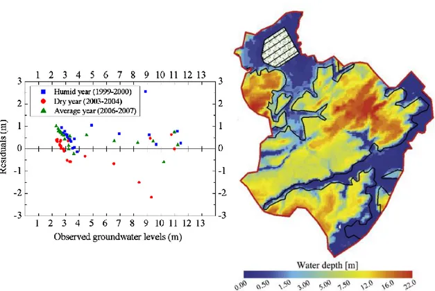
6.2.2. Validation of the calibrated model against wetland vegetation distribution ... 284
6.3. Model sensitivity ... 287
6.3.1. Sensitivity of the initial model to varying depth and shape of the fissured zone .... 287
6.3.2. Systematic sensitivity analysis of the calibrated model ... 291
6.3.3. Sensitivity of the calibrated model to model resolution ... 296
6.3.4. Impact of spatial variation in potential evapotranspiration and peat characteristics ... 301
6.3.5. Sensitivity to the length of the warm-up period and the issue of the overland flow component convergence ... 306
6.4. Model performance and sensitivity: general discussion and recommendations ... 309
6.4.2. Channel flow ... 310
6.4.3. Parametrisation of the unsaturated and saturated peat ... 311
6.4.4. Parametrisation of the unsaturated zone on mineral soils ... 312
6.4.5. Parametrisation of the granite fissured zone ... 313
6.5. Conclusion ... 315
Résumé du chapitre 6 ... 317
Chapter 7. Simulated water balance and hydrological fluxes between the mire and its catchment ... 319
7.1. Introduction ... 319
7.2. Spatial characterisation of the mire hydrology ... 319
7.2.1. Methods ... 319
7.2.2. Results and discussion ... 320
7.3. Water balance ... 326
7.3.1. Methods ... 326
7.3.2. Results and discussion ... 328
7.4. Conclusion ... 338
Résumé du chapitre 7 ... 339
Chapter 8. Impacts of catchment landuse on wetland hydrology ... 341
8.1. Introduction ... 341
8.2. Impacts of catchment landuse on the hydrology of mires ... 341
8.3. Methods ... 343
8.4. Results and discussion ... 345
8.5. Conclusion ... 369
Résumé du chapitre 8 ... 372
Chapter 9. Hydrology and hydrological modelling of acidic mires in the French Massif Central: conclusion and recommendations ... 375
9.1. Concluding review ... 375
9.1.1. Development of a three-dimensional geological model of the mire and its catchment ... 375
9.1.2. Hydrometeorological monitoring ... 377
9.1.3. Conceptual hydrological model ... 378
9.1.4. Numerical hydrological model ... 379
9.1.5. Sensitivity analyses ... 380
9.1.6. Simulated water balance and hydrological fluxes ... 381
9.1.7. Hydrological response to changes in catchment landuse ... 382
9.2.1. Improving the hydrological understanding and modelling of the Dauges site ... 383
9.2.2. Validating research findings using other methodological approaches ... 391
9.2.3. Broadening research questions: the impact of climate change ... 393
9.3. Recommendations for conservation management ... 396
9.3.1. Management of minerotrophic mires in basement regions ... 396
9.3.2. Management of the Dauges National Nature Reserve and Special Area of Conservation ... 398
9.4. Conclusion ... 400
Résumé du chapitre 9 (conclusion) ... 401
References ... 403
Appendix A. Mire classification ... 433
A.1. Hydrogeomorphic classification ... 433
A.1. Hydrogenetic classification ... 434
A.2. Ontogenetic classification ... 439
A.3. Classification based on wetland mechanisms ... 439
A.4. The issue of scale ... 442
Appendix B. Von Post humification index ... 443
Appendix C. Recent advances in hydrogeology of hard-rock regions ... 445
C.1. The stratiform conceptual model of hard-rock aquifers ... 445
C.2. Mapping the depth of weathering profiles ... 451
C.3. Modelling groundwater flow in weathered hardrocks ... 454
Appendix D. Description of pedological pits ... 457
Appendix E. Meteorology: data acquisition and reconstruction of missing and historical time-series ... 465
E.1. Introduction ... 465
E.2. Methods ... 465
E.2.1. Météo-France permanent meteorological stations ... 465
E.2.2. On site ... 466
E.2.3. Time-series reconstruction ... 470
E.3. Results ... 471
E.3.1. Solar radiation ... 471
E.3.2. Temperature ... 474
E.3.3. Relative humidity ... 484
E.3.4. Precipitation ... 494
E.3.5. Wind speed ... 499
E.3.7. In-filled meteorological data ... 506
E.3.8. Representativeness of the model calibration and validation period in terms of climate ... 507
E.4. Conclusion ... 510
Appendix F. Characteristics of dipwells and piezometers installed at the Dauges site ... 511
Appendix G. Published values of evapotranspiration and unsaturated flow parameters ... 513
Appendix H. Differential impacts of open habitats, broadleaf forests and coniferous forests on water yield ... 527
List of figures
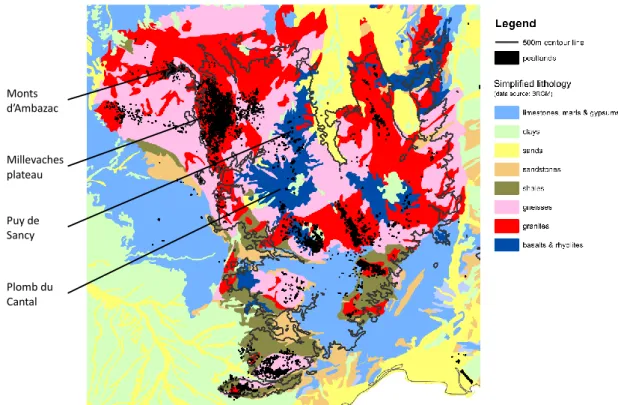
Figure 1-1. Relationship between mire, suo, wetland and peatland (Joosten 2004). ... 39 Figure 1-2. Global distribution of mires (from Lappalainen 1996). ... 40 Figure 1-3. Water retention curves for Sphagnum (a) and reed (b) peats by degree of decomposition (Brandyk et al. 2002). ... 55 Figure 1-4. Relationship between saturated hydraulic conductivity and (a) bulk density or (b) volume of solid matter (from Brandyk et al. 2002). ... 56 Figure 1-5. Peat saturated hydraulic conductivity as a function of botanical composition and von Post's humification index (from Eggelsmann et al. 1993). ... 56 Figure 1-6. Impacts of water table drawdown on peat physical properties and peatland hydrology (from Whittington & Price 2006). ... 60 Figure 1-7. Average contribution of precipitation, surface water and groundwater to the maintenance of summer water levels in English and Welsh mires as a function of (left) identified wetland water supply mechanism and (right) plant community (from Wheeler et al. 2009). ... 62 Figure 1-8. Classification of hydrological models (modified from Thompson, unpublished; Singh 1988; and Jajarmizad et al. 2012). ... 66 Figure 1-9. Workflow in hydrological modelling (modified from Refsgaard 1997). ... 70 Figure 1-10. Performance of the model developed by Lewis et al. (2013) with regard to groundwater table depth (left: calibration, right: validation)... 72 Figure 1-11. Impact of afforestation (including drainage) on simulated groundwater table depth in the blanket bog modelled by Lewis et al. (2013). ... 72 Figure 1-12. Performance of the model developed by Fournier (2008) and Levison et al. (2014) with regard to groundwater table depth. ... 73 Figure 1-13. Exfiltration and throughflow models tested by van Loon et al. (2009). ... 74 Figure 1-14. Correspondance between trophic status estimated from indicator plant species (a) and fraction of exfiltrated groundwater (FEG) in the root zone according to the throughflow model (b) and exfiltration model (c) of van Loon et al. (2009). ... 75 Figure 1-15. The esker-peatland system investigated by Rossi et al. (2012, 2014). ... 76 Figure 1-16. Measured (crosses) vs. simulated (crosses and contour lines) groundwater heads in the upper bedrock aquifer below the Selisoo bog according to Marandi et al. (2013). ... 77 Figure 1-17. Performance of the model developed by Armandine Les Landes et al. (2014) with regard to groundwater table levels (left) and wetland spatial distribution (right). ... 78 Figure 2-1. Distribution of mires in Metropolitan France. ... 85 Figure 2-2. Distribution of peatlands within the Massif Central relative to bedrock lithology. .. 85 Figure 2-3. Proportion of heathland (purple scale) and forest (green scale) in total landcover in Limousin. ... 86 Figure 2-4. Location of the Dauges research catchment and wetland within France (top left), Limousin (top right), and the Monts d'Ambazac massif (bottom right and left). ... 91
Figure 2-5. Three-dimensional view of the Dauges catchment. ... 92
Figure 2-6. View of the Dauges wetland from its north-east boundary (January 2011). ... 92
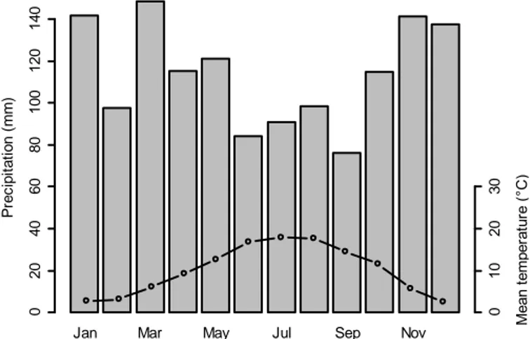
Figure 2-7. Gaussen-Bagnouls ombrothermic diagram of the St-Léger-Mon met station (1998-2010). ... 93
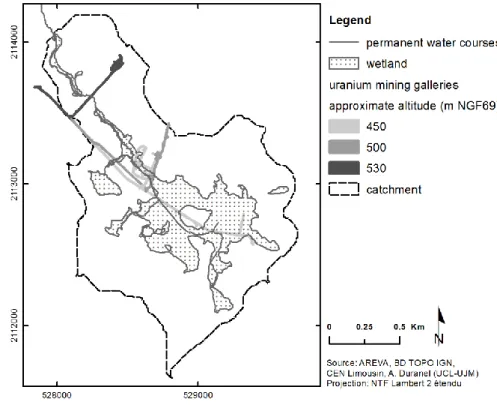
Figure 2-8. Plan projection of uranium mining galleries within the Dauges catchment. ... 94
Figure 2-9. Faults and veins as mapped by GOGEMA. ... 95
Figure 2-10. Landcover within the Dauges catchment. ... 96
Figure 3-1. Distribution density of differences in elevation between the BD topo DEM (after bilinear interpolation) and the DGPS survey points. ... 103
Figure 3-2. Density plot of differences between the DEM (after bilinear interpolation) and DGPS survey points ... 104
Figure 3-3. Topographic data used to build the catchment-wide DEM ... 105
Figure 3-4. Digital Elevation Model of the Dauges wetland. ... 106
Figure 3-5. Location of sections through weathering formations. ... 109
Figure 3-6. Location of boreholes drilled by CEA ... 110
Figure 3-7. Arrangement of electrodes for a 2D electrical resistivity survey using a Wenner array (reproduced from Loke 2000). ... 111
Figure 3-8. Location of ERT transects. ... 113
Figure 3-9. Section 1 - close-up view of the upslope side of the quarry. ... 116
Figure 3-10. Section 2 - Panoramic view of the complete quarry face. ... 117
Figure 3-11. Section 2 - close-up view of the middle of the quarry face. ... 117
Figure 3-12. Section 2 - close-up view of the downslope side of the quarry. ... 118
Figure 3-13. Sections described by Valadas (1998). ... 118
Figure 3-14. Weathering grades and core recovery percentage in the CEA boreholes ... 120
Figure 3-15. Electrical resistivities of the main granite weathering formation according to the literature. ... 121
Figure 3-16. ERT profile 1 (29/10/2012): from top to bottom, measured and calculated apparent resistivity pseudosections, L1-norm inverse model resistivity section. ... 123
Figure 3-17. ERT profile 1 (29/10/2012): L1-norm inverse model resistivity section with topography. ... 124
Figure 3-18. ERT profile 2 (30/10/2012): from top to bottom, measured and calculated apparent resistivity pseudosections, L1-norm inverse model resistivity section. ... 126
Figure 3-19. ERT profile 2 (30/10/2012): L1-norm inverse model resistivity section with topography ... 127
Figure 3-20. ERT profile 3 (03/11/2012): from top to bottom, measured and calculated apparent resistivity pseudosections, L1-norm inverse model resistivity section. ... 129
Figure 3-21. ERT profile 3 (03/11/2012): L1-norm inverse model resistivity section with topography (combined protocols). ... 130
Figure 3-22. ERT profile 4 (04/11/2012): from top to bottom, measured and calculated apparent
resistivity pseudosections, L1-norm inverse model resistivity section. ... 133
Figure 3-23. ERT profile 4 (04/11/2012): L1-norm inverse model resistivity section with topography. ... 134
Figure 3-24. Resistivity as a function of porosity according to Archie's law, for a groundwater electrical conductivity of 27.8 µS.cm-1, with a=1.4 and m=1.58. ... 135
Figure 3-25. Using slope to map outcropping formations ... 138
Figure 3-26. Kernel density estimation of slope distribution in arable land vs. in all dry land. 140 Figure 3-27. Kernel density estimation of slope distribution at mapped rock outcrops vs. in the entire area... 140
Figure 3-28. Nature of the material on which the rod survey stopped. ... 147
Figure 3-29. Peat depth at the Dauges site. ... 148
Figure 3-30. Thickness of easily-penetrable mineral deposits underlying peat at the Dauges site. ... 149
Figure 3-31. Altitude (mNGF69) of the base of peat (top) and mineral (bottom) deposits at the Dauges site. ... 150
Figure 3-32. Stratigraphic profiles. ... 151
Figure 3-33. Acrotelm depth (a) and topographic indices used to model it: terrain slope (b), DInf contributing area (c) and slope over Dinf contributing area ratio (d). ... 153
Figure 3-34. Box- and scatter-plots of acrotelm depth against potential explanatory variables. ... 154
Figure 3-35. Location of slug tests. ... 155
Figure 3-36. Recovery curves following slug tests in peat using temporary piezometers with a 10cm intake... 158
Figure 3-37. Hvorslev model residuals (temporary piezometers in peat). ... 159
Figure 3-38. Recovery curves following slug tests in permanent piezometers. ... 160
Figure 3-39. Hvorslev model residuals (permanent piezometers). ... 161
Figure 3-40. Boxplot of hydraulic conductivities measured in peat using temporary piezometers, according to depth. ... 163
Figure 3-41. Location of pedological pits. ... 164
Figure 4-1. Automatic gauging stations and manual stageboards at the Dauges site. ... 172
Figure 4-2. V-notch weir and float-operated stage logger in its stilling well at Rocher. ... 173
Figure 4-3. Gauging station at the catchment outlet, with the pressure logger in its stilling well.. ... 174
Figure 4-4. Logger drift at the D78 gauging station. ... 176
Figure 4-5. Stream stage at the D78 gauging station. ... 177
Figure 4-6. Scatterplot of stage records at Pont-de-Pierre vs. D78. ... 177
Figure 4-7. D78 stage-discharge scatterplot. ... 178
Figure 4-9. Stream stage at the Pont-de-Pierre gauging station. ... 179
Figure 4-10. Power (left) and polynomial (right) stage-discharge curves at the Pont-de-Pierre gauging station. ... 180
Figure 4-11. Stage-area-mean velocity plots at the Pont-de-Pierre gauging station. ... 181
Figure 4-12. Comparison of stage-discharge curves established with different methods at the Pont-de-Pierre gauging station. ... 182
Figure 4-13. Daily mean discharge at the Pont-de-Pierre gauging station. ... 183
Figure 4-14. Daily mean discharge at the upstream gauging stations. ... 184
Figure 4-15. Manual stage records. ... 185
Figure 4-16. Location of piezometer clusters. ... 186
Figure 4-17. Dipwell and piezometer before installation in the ground. ... 187
Figure 4-18. Movements of selected shallow piezometers relative to an arbitrary datum. ... 190
Figure 4-19. Boxplots of water table height manual reading errors, as estimated by the difference between readings made with the manual dipper and with a tape measure. The right boxplot shows the estimated errors of manual readings used to calibrate logger data. 192 Figure 4-20. Difference between manually- and logger-recorded water table heights before correction for logger drift. ... 193
Figure 4-21. Difference between manually- and logger-recorded water table heights before correction for logger drift, conditional on logger. ... 195
Figure 4-22. Logger data before and after correction for logger drift. ... 196
Figure 4-23. Time series of piezometric heads in clusters 3-6. ... 197
Figure 4-24. Time series of piezometric heads in clusters 7-10. ... 198
Figure 4-25. Time series of piezometric heads in clusters 11-14. ... 199
Figure 4-26. Time series of piezometric heads in clusters 15-18. ... 200
Figure 4-27. Time series of piezometric heads in clusters 19-22. ... 201
Figure 4-28. Time series of piezometric heads in clusters 23-26. ... 202
Figure 4-29. Time-series of water table depth in pre-existing piezometers. ... 203
Figure 4-30. Kernel density estimation of water table depth distribution in the peat layer. .... 204
Figure 4-31. Depth exceedence frequency curves of the water table in the peat layer. ... 205
Figure 4-32. Principal component analysis plots of groundwater table depth records (left: manually-recorded, right: logger-recorded). ... 206
Figure 4-33. Map of dipwell scores on PCA first component. ... 207
Figure 4-34. Piezometric head and stream stage along a transect SB1-D15, downstream of Puy Rond. ... 209
Figure 4-35. Location of dipwells relative to topographic indices: a) DInf catchment area, b) DInf slope over catchment area ratio. ... 211
Figure 4-36. Piezometric heads in cluster 8 and stream stages at stageboard SB3. ... 212
Figure 5-2. Numeric engines available in MIKE SHE for each hydrological process (from Anonymous 2009b). ... 221 Figure 5-3. Allowable water content in the upper layer of the two-layer unsaturated zone model, as a function of water table depth (from Anonymous 2009c). ... 223 Figure 5-4. MIKE 11 branches and MIKE SHE river links (from Anonymous 2009c). ... 226 Figure 5-5. Linkage between MIKE SHE links and MIKE 11 cross-sections (from Anonymous 2009c). ... 226 Figure 5-6. Observed and simulated groundwater table depth in the North Kent marshes (from Thompson et al. 2004). ... 227 Figure 5-7. Observed and simulated groundwater table depth (top) and stream stage (bottom) in Bear Creek Meadow (modified from Hammersmark et al. 2008). ... 228 Figure 5-8. Observed and simulated discharge in the Paya Indah wetlands (Rahim et al. 2012).
... 229 Figure 5-9. Observed and simulated groundwater table level in the Paya Indah wetlands (Rahim et al. 2009). ... 229 Figure 5-10. Performance of the Lanoraie steady-state MIKE SHE model with regard to groundwater head (Bourgault et al. 2014). ... 230 Figure 5-11. Nested models used by Johansen et al. (2014) to model the Lindenborg fen. .... 231 Figure 5-12. Observed and simulated groundwater heads in the Lindenborg fen (Johansen et al. 2014). ... 232 Figure 5-13. Generalised crop coefficient curve (Allen & Pereira 2009) ... 234 Figure 5-14. Idealised crop coefficient curve (Allen et al. 1998)... 236 Figure 5-15. Examples of LAI seasonnal changes in acidic mires. ... 242 Figure 5-16. Leaf area indices used in the model as a function of vegetation class and day of year.
... 242 Figure 5-17. Crop coefficients used in the model as a function of vegetation class and day of year.
... 246 Figure 5-18. Simulated intercepted rainfall fraction in a month as a function of maximum storage capacity (1998-2013). ... 248 Figure 5-19. Ratio of evaporation from interception to maximum potential evapotranspiration as a function of maximum storage capacity (1998-2013). ... 248 Figure 5-20. Maximum interception storage capacities used in the model as a function of vegetation class and day of year. ... 250 Figure 5-21. Simulated fraction of intercepted rainfall in a month as a function of vegetation class (1998-2013). ... 251 Figure 5-22. MIKE 11 hydrographic network. ... 253 Figure 5-23. MIKE 11 cross-sections. ... 254 Figure 5-24. Distribution of peat deposits deeper/shallower than the 0.5m minimum depth of the upper computational layer. ... 257
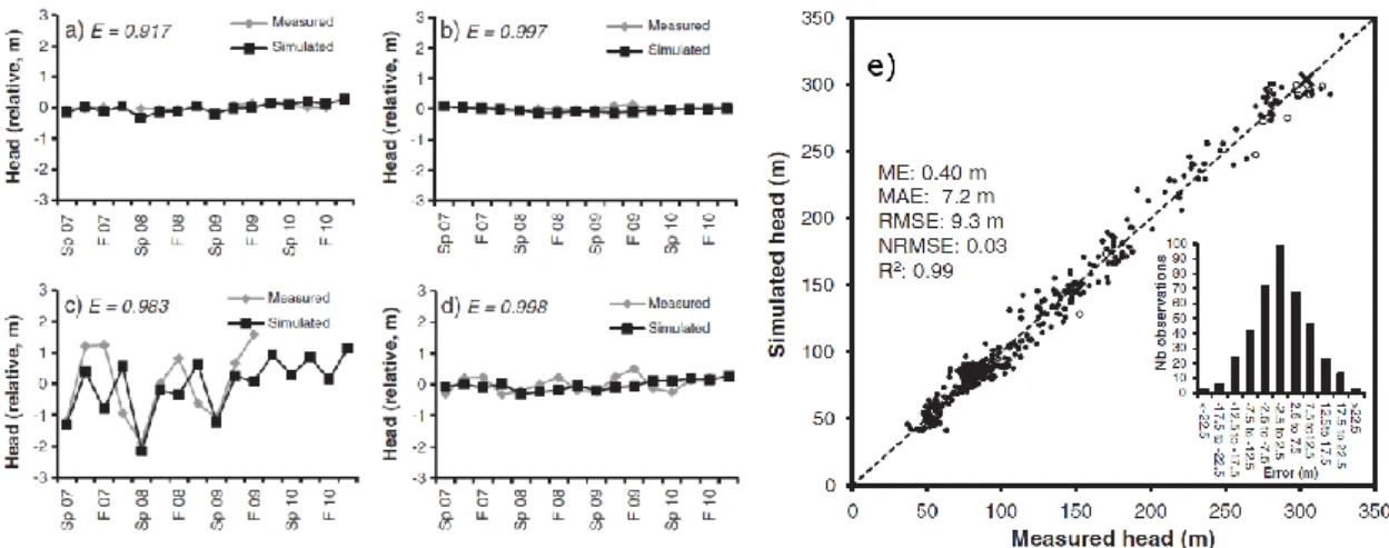
Figure 5-25. Spatial distribution of mean aggregated elevations according to model resolution. ... 260 Figure 5-26. Effect of model resolution and aggregation method on the catchment hypsometric curve (top), elevation density distribution (middle) and slope density distribution (bottom). ... 262 Figure 5-27. Distribution of vegetation classes according to model resolution. ... 263 Figure 5-28. Relative frequency of vegetation classes according to model resolution... 263 Figure 5-29. Effect of the model grid size on the representation of the hydraulic network by the MIKE SHE pre-processor. ... 264 Figure 6-1. Observed and simulated stream discharge (uncalibrated model). ... 270 Figure 6-2. Observed and simulated groundwater table depth (uncalibrated model). ... 271 Figure 6-3. Observed and simulated stream discharge (calibrated model). ... 275 Figure 6-4. Observed and simulated stream stage (calibrated model). ... 276 Figure 6-5. Model performance with regard to groundwater table depth (calibrated model). 277 Figure 6-6. Spatial distribution of shallow groundwater tables (2011-2013 mean higher than -0.286m below ground level) and of wetland vegetation. ... 286 Figure 6-7. Topographic position index (scaled to 0-1 range). ... 289 Figure 6-8. Standardised elevation relative to the modelled palaeosurface elevation. ... 289 Figure 6-9. Systematic sensitivity analysis with respect to groundwater table depth.. ... 294 Figure 6-10. Systematic sensitivity analysis with respect to discharge at Rocher, Marzet and Girolles. ... 295 Figure 6-11. Systematic sensitivity analysis with respect to discharge at Pont-de-Pierre. ... 295 Figure 6-12. Nash-Sutcliffe efficiency for simulated discharge, groundwater table depth and piezometric head as a function of model grid size. ... 297 Figure 6-13. Percent bias in simulated discharge as a function of model grid size. ... 298 Figure 6-14. Effect of model resolution on simulated groundwater table depth. ... 299 Figure 6-15. Effect of local peat specific yield, peat available water capacity and wetland crop coefficient on simulated groundwater table depth. ... 303 Figure 6-16. Effect of the simulation period on simulated discharge at Marzet and Pont-de-Pierre.
... 306 Figure 6-17. Simulated discharge at Marzet with a simulation period from 01/08/1998 to 31/12/2013. ... 307 Figure 6-18. Overland flow component accumulated error (2011-2013) as a function of the total length of the simulation period. ... 307 Figure 6-19. Mean simulated overland depth (2011-2013) as a function of the total length of the simulation period. ... 308 Figure 7-1. Simulated mean groundwater table depth, upward groundwater flow from lower to upper computational layers and seepage from saturated zone to overland flow (01/01/2011-31/12/2013). ... 321
Figure 7-2. Simulated mean upward groundwater flow from lower to upper computational layers (01/01/2011-31/12/2013). ... 323 Figure 7-3. Simulated mean seepage from saturated zone to overland flow
(01/01/2011-31/12/2013). ... 323 Figure 7-4. Simulated monthly mean groundwater table depth (01/01/2011-31/12/2013). .. 324 Figure 7-5. Simulated monthly mean vertical groundwater flow between computational layers (01/01/2011-31/12/2013). ... 325 Figure 7-6. Simulated monthly mean seepage from saturated zone to overland flow
(01/01/2011-31/12/2013). ... 326 Figure 7-7. Water balance sub-catchments. ... 327 Figure 7-8. Simulated water balance of the mire area upstream of Pont-de-Pierre from 01/01/2011 to 31/12/2013 (m3). ... 329
Figure 7-9. Simulated monthly water balance of the mire upstream of Pont-de-Pierre. ... 331 Figure 7-10. Simulated monthly water balance of the mire interception and overland flow components. ... 332 Figure 7-11. Simulated monthly water balance of the mire unsaturated zone component. .... 333 Figure 7-12. Simulated monthly water balance of the mire saturated zone component (upper computational layer only). ... 334 Figure 7-13. Relative importance of individual evapotranspiration components in simulated monthly actual evapotranspiration (mire upstream of Pont-de-Pierre, 01/01/2011-31/12/2013). ... 335 Figure 7-14. Relative importance of individual components in simulated monthly inflow to the mire (upstream of Pont-de-Pierre, 01/01/2011-31/12/2013). ... 335 Figure 7-15. Relative importance of individual components in simulated monthly inflow to the mire saturated zone (upstream of Pont-de-Pierre, 01/01/2011-31/12/2013). ... 336 Figure 8-1. Distribution of vegetation classes in the catchment landuse scenarios. ... 344 Figure 8-2. Simulated impacts of catchment landuse on the catchment monthly water balance (absolute changes relative to baseline, 01/01/2011-31/12/2013)... 346 Figure 8-3. Simulated impacts of catchment landuse on the mire monthly water balance (absolute changes relative to baseline, 01/01/2011-31/12/2013)... 348 Figure 8-4. Impacts of catchment landuse on monthly water balance errors
(01/01/2011-31/12/2013). ... 350 Figure 8-5. Simulated impacts of catchment landuse on evapotranspiration components within the catchment (01/01/2011-31/12/2013). ... 351 Figure 8-6. Impacts of catchment landuse on simulated daily discharge at the four discharge monitoring stations (01/01/2011-31/12/2013). ... 357 Figure 8-7. Impacts of catchment landuse on simulated flow exceedence frequency curves at the four discharge monitoring stations (01/01/2011-31/12/2013). ... 358 Figure 8-8. Impacts of catchment landuse on simulated groundwater table depth in a selection of dipwells within the mire (01/01/2011-31/12/2013). ... 360
Figure 8-9. Impacts of catchment landuse on simulated groundwater table depth exceedence frequency curves in a selection of dipwells within the mire (01/01/2011-31/12/2013). ... 361 Figure 8-10. Spatial distribution of change in simulated monthly mean groundwater table depth under the conifer scenario, relative to the baseline (01/01/2011-31/12/2013). ... 363 Figure 8-11. Spatial distribution of change in simulated monthly mean groundwater table depth within the mire under the conifer scenario, relative to the baseline (01/01/2011-31/12/2013). ... 364 Figure 8-12. Spatial distribution of change in simulated monthly mean groundwater table depth under the grassland scenario, relative to the baseline (01/01/2011-31/12/2013). ... 367 Figure 8-13. Spatial distribution of change in simulated monthly mean groundwater table depth within the mire under the grassland scenario, relative to the baseline (01/01/2011-31/12/2013). ... 368 Figure 9-1. Mean anomaly in reference evapotranspiration (FAO Penman-Monteith) simulated by the SCAMPEI and SCRATCH08 GCM downscaling experiments for the Dauges area. 394 Figure 9-2. Mean anomaly in monthly precipitation simulated by the SCAMPEI and SCRATCH08 GCM downscaling experiments for the Dauges area... 394 Figure 9-3. Comparison of reference evapotranspiration and precipitation observed at the Dauges site with those simulated by the SCAMPEI and SCRATCH08 downscaling experiments for the nearest grid cell. ... 395
Figure A-1. Cross-sections and plan views of key hydrogeomorphic mire types (from Charman 2002). ... 433 Figure A-2. Sub-types of horizontal mires (from Schumann & Joosten 2008) ... 435 Figure A-3. Percolation mire (from Schumann & Joosten 2008). ... 436 Figure A-4. Surface flow mires (from Schumann & Joosten 2008). ... 437 Figure A-5. Acrotelm mire (from Schumann & Joosten 2008). ... 437 Figure A-6. Gilvear’s & McInnes’ (1994) wetland classification scheme (from Gilvear & Bradley 2009). ... 440 Figure C-1. Classical conceptual hydrogeological model of hard-rock aquifers (translated from Lachassagne et al. 2009). ... 445 Figure C-2. Conceptual hydrogeological model of stratiform hard-rock aquifers (from Wyns et al. 2004). ... 448 Figure C-3. Age of weathering formations in Limousin (translated from Mauroux et al. 2009).
... 451 Figure C-4. Formation of the present-day landscape from the infra-Cretaceous planation surface (from Lachassagne et al. 2001b). ... 452 Figure C-5. Reconstitution of palaeosurfaces (from Lachassagne et al. 2001b). ... 452 Figure E-1. Influence of computation method on daily temperature and relative humidity extremes. ... 469 Figure E-2. Theoretical clear-sky and measured daily global radiations at the Dauges site. .... 471
Figure E-3. Daily global and reflected radiations and their ratio at the Dauges site, inferred presence of snow on the ground. ... 472 Figure E-4. Double mass curve of global shortwave radiation at the Dauges site and at the two nearest Météo-France stations. ... 473 Figure E-5. Scatterplots of global shortwave radiation at the Dauges site and at the two nearest Météo-France stations. ... 474 Figure E-6. Observed vs. predicted daily global shortwave radiation at the Dauges site. ... 474 Figure E-7. Scatterplot of air temperatures measured with the Hobo and Enerco loggers at the Dauges site. ... 475 Figure E-8. Scatterplots of temperature extremes recorded by the Enerco and Hobo loggers at the Dauges site. ... 476 Figure E-9. Daily temperature extremes at the Dauges site. ... 476 Figure E-10. Scatterplots of daily maximum temperatures at the Dauges site against records at nearby Météo-France stations. ... 477 Figure E-11. Scatterplots of daily minimum temperatures at the Dauges site against records at nearby Météo-France stations. ... 477 Figure E-12. Scatterplots of daily temperature extremes at the bottom of the wetland and at
mid-slope (Les Ribières) at the Dauges site. ... 478 Figure E-13. Temperatures measured at the bottom of the wetland and in the upper part of the catchment (Les Ribières) at the Dauges site. ... 478 Figure E-14. Scatterplots of daily temperature extremes at mid-slope (Les Ribières) and at
St-Léger-Mon. ... 479 Figure E-15. Scatterplots of the anomaly in daily minimum temperature at the Dauges site against other meteorological variables. ... 480 Figure E-16. Correlation matrix of potential variables to be included in a model of daily minimum temperatures at the Dauges site. ... 481 Figure E-17. Observed vs. predicted daily minimum temperatures at the Dauges site. ... 483 Figure E-18. Observed vs. predicted daily maximum temperatures at the Dauges site. ... 484 Figure E-19. Uncorrected hourly relative humidity measured by the Enerco and Hobo loggers at the Dauges site. ... 485 Figure E-20. Uncorrected and corrected relative humidity data from the Enerco logger using two different methods. ... 487 Figure E-21. Scatterplot of corrected Enerco-recorded vs. Hobo-recorded hourly relative humidity at the Dauges site. ... 488 Figure E-22. Scatterplots of relative humidity daily extremes recorded by the Enerco and Hobo loggers at the Dauges site. ... 488 Figure E-23. Daily minimum and maximum relative humidity at the Dauges site. ... 489 Figure E-24. Scatterplots of daily minimum relative humidity at the Dauges site and at nearby Météo-France stations. ... 489 Figure E-25. Scatterplots of daily maximum relative humidity at the Dauges site and at nearby Météo-France stations. ... 490
Figure E-26. Scatterplots of daily temperature extremes at the bottom of the wetland and at mid-slope (Les Ribières) at the Dauges site. ... 491 Figure E-27. Scatterplots of daily relative humidity extremes at les Ribières and at nearby
Météo-France stations. ... 491 Figure E-28. Predicted vs. observed daily minimum relative humidity at the Dauges site. ... 493 Figure E-29. Predicted vs. observed daily maximum relative humidity at the Dauges site. ... 494 Figure E-30. Scatterplots of hourly and daily precipitation recorded by the Enerco and PM3030 raing gauges at the Dauges site. ... 495 Figure E-31. Double mass curves (left) and cumulative curves (right) of precipitation records at the Dauges site and at nearby Météo-France stations. ... 495 Figure E-32. Impact of snow fall events on the difference between precipitation records at the Dauges site and at the Saint-Léger-la-Montagne station. ... 496 Figure E-33. Daily precipitation at the Dauges site. ... 497 Figure E-34. Scatterplots of precipitation records at the Dauges site against records at nearby Météo-France stations. ... 497 Figure E-35. Scatterplot of precipitation at the two Météo-France rain gauges in
Saint-Léger-la-Montagne. ... 498 Figure E-36. Observed vs. predicted daily precipitation at the Dauges site. ... 499 Figure E-37. Daily mean wind speed at the Dauges site. ... 500 Figure E-38. Scatterplots of daily mean wind speed records at the Dauges site against those at nearby Météo-France stations. ... 500 Figure E-39. Predicted vs. observed daily mean wind speed at the Dauges site. ... 501 Figure E-40. Reference evapotranspiration at the Dauges site computed using different methods.
... 502 Figure E-41. Scatterplot matrix of reference evapotranspiration at the Dauges site computed using different methods. ... 503 Figure E-42. Scatterplot matrix of different potential evapotranspiration estimations using temperature records from the wetland and from the nearby Météo-France station at Saint-Léger-la-Montagne. ... 504 Figure E-43. Scatterplots of reference evapotranspiration derived from observed vs. modelled meteorological time-series at the Dauges site. ... 506 Figure E-44. Scatterplots of reference evapotranspiration derived from observed meteorological data at the Dauges site vs. at Limoges-Bellegarde. ... 506 Figure E-45. Observed and in-filled meteorological time-series at the Dauges site. ... 508 Figure E-46. Standardised Precipitation-Evapotranspiration Index (1998-2013). ... 509 Figure H-1. Maximum change in annual flow following deforestation or afforestation in 137 paired-catchment experiments (from Andréassian 2004). ... 527
List of tables
Table 1-1. Correspondance between humification classes and humification indicators (Szajdak et al. 2011). ... 54 Table 1-2. Bulk density, total porosity and specific yield measured in northern Minnesota bogs (Boelter 1968). ... 54 Table 1-3. Percent of runoff collected in automated throughflow troughs from peat layers in an undisturbed blanket bog hillslope, UK (Holden 2006). ... 64 Table 2-1. Total area and frequency of vegetation classes within the Dauges catchment. ... 95 Table 3-1. Position of the survey benchmark. ... 102 Table 3-2. Characteristics of ERT transects completed at the Dauges site. ... 113 Table 3-3. Water electrical conductivity in the main stream at the Dauges site. ... 135 Table 3-4. Hydraulic conductivities (m.s-1) measured at different depths in peat using temporary
piezometers. ... 163 Table 3-5. Hydraulic conductivities (m.s-1) measured in peat and underlying mineral formations
using permanent dipwells and piezometers. ... 163 Table 4-1. Amplitude of piezometer movements. ... 191 Table 5-1. Unsaturated zone parameters. ... 238 Table 5-2. Mean bud break and leaf colouring day-of-year and date estimated for deciduous broadleaved species at the Dauges site based on figures from Lebourgeois et al. (2010). ... 240 Table 5-3. Mean tree height in the Plateaux Limousins eco-region according to IFN data. ... 244 Table 5-4. Simulated bulk interception ratio as a function of maximum storage capacity
(1998-2013). ... 249 Table 5-5. Simulated fraction of intercepted rainfall (1998-2013). ... 251 Table 5-6. Vegetation properties used in the Dauges model. ... 252 Table 5-7. Summary of initial parameter values used in the model. ... 259 Table 6-1. Calibrated parameters. ... 274 Table 6-2. Confusion matrix (% of the total number of pixels). ... 285 Table 6-3. Nash-Sutcliffe Efficiency before calibration as a function of the shape and depth of the fissured zone ... 291 Table 6-4. Parameters included in the systematic sensitivity analysis. ... 293 Table 6-5. Effect of unsaturated peat specific yield, unsaturated peat available water capacity and wetland crop coefficient during the vegetation season on the Nash-Sutcliffe Efficiency for individual dipwells. ... 302 Table 7-1. Simulated water balances of the mire, of its catchment and of both areas combined from 01/01/2011 to 31/12/2013. ... 330 Table 8-1. Frequency of vegetation classes within the wetland, catchment and combined water balance computation areas (baseline). ... 344
Table 8-2. Simulated impacts of catchment landuse on catchment and mire overall water balances (01/01/2011-31/12/2013). ... 345 Table 8-3. Change (and percent change in brackets) in simulated stream flow quantiles and mean flow (l.s-1) under conifer and grassland catchment landuse scenarios relative to the
baseline (01/01/2011-31/12/2013). ... 358 Table 8-4. Impacts of catchment landuse on the number of days per year with a simulated groundwater table depth deeper than 0, -0.1 and -0.2m below ground in a selection of dipwells within the mire (01/01/2011-31/12/2013). ... 362
Table A-1. Hydrogenetic mire types (modified from Joosten & Clarke 2002). ... 438 Table A-2. Descriptors of the wetland framework (Wheeler et al. 2009). ... 441 Table A-3. Wetland Water Supply Mechanisms (WETMECs, Wheeler et al. 2009; Whiteman et al. 2009). ... 442 Table B-1. Von Post humification index (adapted from Soil Classification Working Group 1998; Quinty & Rochefort 2003; Parent & Caron 2008) ... 443 Table C-1. Variation of hydraulic conductivity with depth in a leucogranite in St-Sylvestre (Bertrand & Durand 1983). ... 449 Table C-2. Conceptual models of flow in fractured/fissured media (modified from Singhal & Gupta 2010). ... 454 Table D-1. Position of pedological pits ... 457 Table E-1. Météo-France permanent meteorological stations close to the Dauges site. ... 465 Table E-2. Availability of meteorological data at Météo-France stations close to the Dauges site.
... 466 Table E-3. Definition of meteorological variables provided by Météo-France. ... 466 Table E-4. 24-hour periods used by Meteo-France to aggregate meteorological variables. .... 466 Table E-5. Definition of variables measured at the Dauges site. ... 467 Table E-6. Coefficients of the minimal model for global radiation at the Dauges site. ... 474 Table E-7. Coefficients of the minimal model for daily minimum temperature at the Dauges site.
... 482 Table E-8. Coefficients of the minimal model for daily maximum temperature at the Dauges site.
... 483 Table E-9. Correlation of corrected humidity data at the Dauges site with control datasets. .. 487 Table E-10. RMSE of corrected relative humidity data at the Dauges site with control datasets.
... 487 Table E-11. Coefficients of the minimal model for daily minimum relative humidity at the Dauges site. ... 492 Table E-12. Coefficients of the minimal model for daily maximum relative humidity at the Dauges site. ... 493 Table E-13. Coefficients of the minimal model for daily precipitation at the Dauges site. ... 498 Table E-14. Coefficients of the minimal model for daily mean wind speed at the Dauges site. 501
Table E-15. Mean annual precipitation and reference evapotranspiration at the Dauges site. 507 Table F-1. Characteristics of dipwells and piezometers installed at the Dauges site. ... 511 Table G-1. Literature review of crop coefficients relevant to the Dauges site. ... 514 Table G-2. Literature review of leaf area index (LAI) values used in hydrological modelling or measured in contexts similar to the Dauges site. ... 517 Table G-3. Literature review of rooting depth values used in hydrological modelling or measured in contexts similar to the Dauges site. ... 519 Table G-4. Literature review of mean leaf resistance (rl) values used in hydrological modelling or
measured in contexts similar to the Dauges site. ... 520 Table G-5. Literature review of bulk interception ratios measured in contexts similar to the Dauges site. ... 522 Table G-6. Literature review of maximum and specific storage capacities measured in contexts similar to the Dauges site. ... 524
Remerciements
I am particularly indebted to Dr Julian Thompson, my primary supervisor at UCL, for giving me the opportunity to undertake the research project I had long dreamed of. His encouragements after each of our meetings, his extraordinarily patient help with the intricacies of MIKE SHE and his meticulous editing of my approximate Frenglish have been invaluable.
I am grateful to Dr Helene Burningham, my secondary supervisor at UCL, for her help with image processing, GIS and DGPS; and always pertinent advice during our meetings.
Le travail de terrain effectué pendant cette thèse n’aurait été ni financièrement ni techniquement possible sans l’aide de mon directeur de thèse à l’Université Jean Monnet de Saint-Etienne, le Professeur Hervé Cubizolle, directeur du laboratoire EVS-ISTHME UMR5600 CNRS, et cette thèse aurait été entièrement différente sans son implication. Son enthousiasme pour mon projet, sa connaissance du financement de la recherche en France, son soutien inconditionnel et son amitié ont été précieux.
Je suis également très reconnaissant aux multiples personnes qui m’ont aidé pendant ce projet : Mes vieux (et pas si vieux) collègues du Conservatoire des Espaces Naturels du Limousin et de la Réserve Naturelle Nationale de la Tourbière des Dauges : Philippe Durepaire, Karim Guerba, Murielle Lancroz, Anaïs Lebrun, Véronique Lucain, pour avoir réalisé une bonne partie des relevés manuels hydrologiques et météorologiques décrits dans cette thèse, pour s’être pliés avec bonne volonté à mes demandes répétées pour toujours plus de données et toujours plus de précision dans leur collecte, et pour leur accueil. Ce fut un grand plaisir que de passer ces nombreuses semaines de terrain à leurs côtés. Erwan Hennequin, Guy Labidoire, et à nouveau P. Durepaire, M. Lancroz et A. Lebrun, pour m’avoir aidé à porter ces lourdes batteries au plomb et ces cables électriques dans la tourbière inondée lors des relevés de tomographie de résistivité électrique. Je suis certain que peu de personnes ont eut cette expérience, et tout aussi certain que ceux qui l’ont vécue savent les sacrifices que vous avez consentis pour la Science! Véronique Daviaud et Céline Gombert, pour leur aide avec les prélèvements de tourbe et l’expérimentation de la méthode du PVC respectivement. A nouveau G. Labidoire, mon coupeur de bambou préféré! Et enfin Fred Yvonne, Maïwenn Lefrançois, Cécilia Ferté et Pierre Seliquer.
Dr Robert Wyns (Bureau de Recherches Géologiques et Minières), pour l’intérêt qu’il a bien voulu porter à mon travail, sa disponibilité et ses précieux conseils sur les formations d’altération du granite. Cette thèse aurait omis de nombreux points cruciaux sans son aide. Dr Stéphane Garambois, Isabelle Douste-Bacqué, Julien Turpin (Institut des Sciences de la Terre, Grenoble), pour m’avoir permis d’utiliser leur matériel de tomographie et pour leur aide avec l’interprétation des données.
The many members of staff of the UCL Department of Geography that have provided scientific advice or technical help: Prof John French, Dr Mat Disney, Dr Vivienne Jones, Prof Anson Mackay, Prof Neil Rose, Prof Richard Taylor, Dr Handong Yang, Dr Gavin Simpson, Dr Simon Turner, Ajay Chauhan, Catherine D’Alton, Susan Hennessy, Janet Hope, Miles Irving, Tom Knight, Nick Mann, Ian Patmore, Kevin Roe, Tula Maxted, Dr Suse Keay, Maria Rodriguez. And also Amanda Green, Hannah Clilverd, Andrew House, Mohammed Rahman, Luca Marazzi, Luke Mitchell, Miriam Fernandez-Nunez, Charlie Stratford and Lizzie Gardner, some of my fellow PhD students, for mutual (or not!) help and always interesting discussions.
Rashed Khandker (UCL Bartlett), Liz Jones (UCL CEGE), Dr Katherine Holt, Dr Tom Varley (UCL Chemistry), Stuart Laidlaw (UCL Archaeology), for help with scanners, DGPS, IR spectrometers and cameras respectively.
Alain Chomiack (DREAL Limousin), pour son aide avec l’installation des deux enregistreurs à pression à l’aval de la tourbière. Bruno Gratia (Ecole Forestière de Meymac), pour la réalisation des fosses pédologiques. Colin Roberts, Charlie Stratford, Dr James Sorensen, Prof Mike Acreman (Centre for Ecology & Hydrology), for their help at Boxford and with questions relative to hydrological monitoring. Corinne Bauvet, Grégory Agnello (Evinerude), Dr Pierre Goubet (cabinet Sphagnum), Vincent Hugonnot (Conservatoire Botanique National du Massif Central), pour l’identification d’échantillons de bryophytes et lichens. Audrey Gibeaux (AREVA), pour m’avoir permis d’accéder aux archives d’AREVA. Gwen Hitchcock (Wildlife Trust for Bedfordshire, Cambridgeshire & Northamptonshire), Lisa Lane (Berkshire, Buckinghamshire and Oxfordshire Wildlife Trust), for granting access to the nature reserves they manage. Nicolas Saelen (Précis-Mécanique), pour ses conseils sur le matériel de suivi météorologique. Les membres du laboratoire EVS-ISTHME UMR 5600 CNRS, UJM, en particulier le Professeur Bernard Etlicher, pour la journée qu’il a très aimablement consacrée à m’expliquer sur le terrain les formations et processus péri-glaciaires, et pour la relecture qu’il a faite de certains chapitres de cette thèse ; mais aussi Dr Pierre-Olivier Mazagol, Renaud Mayoud, Dr Jérôme Porteret, Carole Bessenay,
Catherine Guillot, Dr Céline Sacca et Axel Mure. Dr Véronique Lavastre (Département de Géologie, UJM), pour ses conseils et son aide concernant l’analyse des sol. Cédric Tavaud (SYMILAV), pour l’intérêt qu’il a porté à mon travail, et le temps et les efforts qu’il a bien voulu y consacrer lors relevés de tomographie à Gourgon ; ainsi que Xavier de Villele, pour avoir mis à ma disposition le matériel du syndicat et un peu du temps de son personnel. Annick Auffray (Météo-France), pour m’avoir fourni de nombreuses données météorologiques. Dr Gilles Thébaud (Herbiers Universitaires de Clermont-Ferrand), pour ses conseils sur l’identification et la cartographie des communautés végétales tourbeuses. Dr Vincent Gaertner, Dr Kristell Michel, Dr Marie-Laure Trémélo (UMR 5600 EVS), pour m’avoir permis d’utiliser le matériel de l’UMR. Vincent Magnet, Cathy Mignon-Linet (Parc Naturel Régional de Millevaches en Limousin), pour leur aide avec la demande de subvention initiale. Dr Jean-Claude Linet, pour son accueil. Tu restes dans nos pensées. Prof Frank Chambers (University of Gloucestershire), for his enthusiasm for the PhD project I submitted to him. Sorry for choosing UCL after all! Ivan and Jacqueline Wright, for their help with microscope calibration. James Giles (Natural England), for allowing access to Thursley Common NNR. Dr Stephan Hennekens (Alterra), for graciously allowing me to use TurboVeg and for his help with the software.
Armelle Denis, Renaud Colin et Benoit Rossignol (Etablissement Public Loire), pour leur aide avec les demandes de subvention , et pour m’avoir invité à présenter mon travail à Bruxelles, Limoges et Clermont-Ferrand. Samuel André, pour m’avoir permis d’obtenir un financement de l’Agence de l’Eau Loire Bretagne.
Les personnes ayant participé à la réunion d’octobre 2009 à St-Gence, France: Dr L. Chabrol (Conservatoire Botanique National du Massif Central), E. Hennequin, P. Durepaire, P. Seliquer, M. Bonhomme et K. Guerbaa (Conservatoire des Espaces Naturels du Limousin), V. Magnet (Parc Naturel Régional de Millevaches en Limousin), Prof M. Botineau (Laboratoire de Botanique et Cryptogamie de la Faculté de Pharmacie de Limoges & Conseil Scientifique Régional de Protection de la Nature), Prof B. Valadas et Prof P. Allée (GéoLab, Universités de Limoges-Clermont), Dr R. Nicolau (Ecole Nationale Supérieure d'Ingénieurs de Limoges), Dr Yoann Brizard (Syndicat d'Aménagement du Bassin de la Vienne Moyenne), Samuel André (Agence de l’Eau Loire Bretagne). L’intérêt marqué dont ils ont fait preuve pour mon projet ainsi que le rappel à la réalité qu’ils m’ont gentiment proposé ont été grandement appréciés.
Gaëlle, Geneviève et Alain (Auberge de St-Martin-des-Olmes). Votre Hotel de Jeunesse est un vrai joyau, ce fut un grand plaisir que d’y passer ces quelques semaines!
Yvan et Elodie, Fred, Arnaud, Michel et Sylvie, Guy et Noëlle, pour leur écoute et pour m’avoir permis de souffler un peu en leur inestimable compagnie.
Jacques et Yvonne, pour leur soutien continu. Marie-Claude, pour avoir suppléé à mes obligations paternelles en de si nombreuses occasions et avec tant de bonne volonté lorsque je désertais la maison familiale pour aller égoistement me “promener” dans les tourbières du Massif Central.
Vincent et Simon, mes bonhommes, pour être venus à ma rescousse tant de fois en demandant “Daddy, can I watch pirates / dinosaurs / Peppa Pig / des chevaliers / castles / des camions de pompier / bin lorries / des requins / whales / un lion / planes… on your computer?” quand vous réalisiez qu’un script sur R commençait à me désespérer.
Sandrine, ce travail n’existerait tout simplement pas sans le soutien inconditionnel, la patience, la compréhension, les encouragements et l’amour dont tu as fait preuve tout au long de celui-ci. De tout coeur, merci.
Ce travail a bénéficié du soutien financier des organisations suivantes : Natural Environment Research Council studentship (UK), Fond Européen de Développement Régional (EU), Agence de l’Eau Loire Bretagne (F), Conservatoire des Espaces Naturels du Limousin (F), EVS-ISTHME UMR5600 CNRS Université Jean Monnet Lyon-St-Etienne (F). Les financements obtenus auprès des institutions européennes et françaises l’ont été dans le cadre du Plan Loire Grandeur Nature, géré par l’Etablissement Public Loire (http://www.plan-loire.fr), grâce à une collaboration entre le Département de Géographie d’UCL et le laboratoire EVS-ISTHME UMR5600 CNRS Université Jean Monnet Lyon-St-Etienne.
Copyright permissions
I am grateful to the following people and organisations for granting permission to reproduce copyright material: Bureau de Recherches Géologiques et Minières (Figure C-3), DHI (Figures 5-2 to 5-5), Elsevier (Figures 1-13, 1-14, 1-17, 5-6, 5-15 and H-1), Geological Society of Malaysia (Figure 5-9), International Association of Hydrological Sciences (Figure C-1), International Peatland Society (Figure 2), IWA Publishing (Figure 5-10), John Wiley and Sons (Figures 5, 1-6, 1-10, 1-11, 1-12, 5-7, 5-8, 5-11, 5-12, 5-15, 5-15, A-1, A-1-6, C-4 and C-5), Prof. Dr. Dr. h.c. Hans Joosten & International Mire Conservation Group (Figures 1-1 and A-2 to A-5), Dr M.H. Loke – Geotomosoft Solutions (Figure 3-7), Springer (Figures 1-15, 1-16 and 5-13), Taylor and Francis Group LLC Books (Figures 1-3, 1-4 and 5-1).
Acronyms and abbreviations
3D three-dimensional
APPB arrêté préfectoral de protection de biotope
asl above sea level
AWC available water capacity
bdin boundary inflow
bdout boundary outflow
BRGM Bureau de Recherches Géologiques et Minières
cal. BP calibrated radiocarbon years before the present
CEA Commissariat à l'Energie Atomique CEN Conservatoire des Espaces Naturels COGEMA Compagnie Générale des Matières
Atomiques
DEM digital elevation model
df degree of freedom
DGPS differential global positioning system
DOC dissolved organic carbon
err error
ERT electrical resistivity tomography Eto reference evapotranspiration
EU European Union
evap evaporation
FAO Food and Agriculture Organisation
FFM daily mean wind speed
GAM generalised additive model
GCM global climate model
GIS geographic information system
GLO daily global shortwave radiation GLS generalised least square
GNSS global navigation satellite system GPS global positioning system
GWT groundwater table
IGN Institut Géographique National infilt infiltration
int interception
Kc crop coefficient
L2E Lambert II étendu
LAI leaf area index
LM linear model
MAE mean absolute error
ME mean error
MY million years
neg negative
NGF nivellement général de la France
NNR national nature reserve
NSE Nash-Sutcliffe efficiency
NTF nouvelle triangulation de la France NVC national vegetation classification
OL overland
OLS ordinary least square
PBIAS percent bias
PCA principal component analysis percol percolation
pos positive
RGF réseau géodésique français
riv river
RMSE root mean square error
RR precipitation
RSR RMSE-observations standard
deviation ratio
RTK real-time kinematic
SAC special area of conservation
SD standard deviation
SEV sum exceedence value
SHE système hydrologique européen
sto storage
Sy specific yield
SZ saturated zone
T transpiration
TM daily mean temperature
TN daily minimum temperature
TPI topographic position index transp transpiration
TX daily maximum temperature
UN daily minimum relative humidity
UTC coordinated universal time
UX daily maximum relative humidity
UZ unsaturated zone
VES vertical electrical sounding
WGS world geodesic system
Chapter 1. Hydrology and hydrological modelling of mires
1.1. Introduction
This thesis investigates the hydrology of the Dauges National Nature Reserve (NNR), an acidic mire in the Monts d’Ambazac, on the western side of the French Massif Central. The research is based on a combination of hydrological and hydrogeological surveys, monitoring and modelling using MIKE SHE / MIKE 11, a distributed physically-based hydrological/hydraulic model. The Massif Central is one of the areas with the highest density of mires in Metropolitan France. As a consequence of the high value of these environments for nature conservation, and also of the many environmental services they provide, a large number are protected under both the national and European legislation. The current chapter provides an introduction to the thesis by reviewing relevant scientific literature on mires, mire hydrology and mire hydrological modelling. Specific details of the mires in the Massif Central are presented in Chapter 2 before the mire of the Dauges NNR and its catchment are introduced and the aims and objectives of the research undertaken in this site are presented.
1.2. Peat, peatlands and mires
1.2.1. Definitions
According to the International Mire Conservation Group (Joosten & Clarke 2002; Schumann & Joosten 2008), peat is a sedentarily accumulated material consisting of at least 30% (dry mass) of dead organic material. Peat soils (often called histosols) are generally defined by the presence of a minimum depth of peat (or histic horizon). However the thresholds in both organic content used to define peat and peat depth used to define histosols vary widely in the wetland and soil sciences literature (Chesworth 2008). For instance, the minimum organic content defining peat varies from 20% to 80% (Rydin & Jeglum 2006). The FAO defines a histic horizon as having at least 20-30% organic content, being saturated with water for at least 30 days in most years (unless artificially drained), and having a thickness of at least 10cm. The French Référentiel
Pédologique (Baize & Girard 2009) uses thresholds of 50% of organic matter and 10cm depth.
According to Joosten & Clarke (2002), the organic matter threshold of 30% is the most frequently encountered in definitions of peat and organic soil in the international literature and is that adopted by both the International Mire Conservation Group and the International Peat Society. As defined by Joosten & Clarke (2002), peat is an organic material that has formed on the spot