Mohamed Ali Jemmali1, Martin J.-D. Otis2* and Mahmoud Ellouze3
1 University of Ottawa, Ontario, Canada, [email protected]
2* LAR.i Lab, University of Quebec at Chicoutimi, Quebec, Canada [email protected]
3 École Nationale d’Ingénieurs de Tunis, Université de Tunis El Manar, [email protected]
Abstract
Purpose
Nonlinear systems identification from experimental data without any prior knowledge of the system parameters is a challenge in control and process diagnostic. It determines mathematical model pa-rameters that are able to reproduce the dynamic behavior of a system. This paper combines two fun-damental research areas: MIMO state space system identification and nonlinear control system. This combination produces a technique that leads to robust stabilization of a nonlinear Takagi-Sugeno fuzzy system (T-S).
Design/methodology/approach
The first part of this paper describes the identification based on the Numerical algorithm for Subspace State Space System IDentification (N4SID). The second part, from the identified models of first part, explains how we use the interpolation of Linear Time Invariants (LTI) models to build a nonlinear multiple model system, T-S model. For demonstration purposes, conditions on stability and stabiliza-tion of discrete time, Takagi-Sugeno (T-S) model were discussed.
Findings
Stability analysis based on the quadratic Lyapunov function to simplify implementation was ex-plained in this paper. The LMIs (Linear Matrix Inequalities) technique obtained from the linearization of the BMIs (Bilinear Matrix Inequalities) was computed. The suggested N4SID2 algorithm had the smallest error value compared to other algorithms for all estimated system matrices.
Originality
The stabilization of the closed-loop discrete time T-S system, using the improved PDC control law (Parallel Distributed Compensation), was discussed to reconstruct the state from nonlinear Luen-berger observers.
1. Introduction
Recent research was developed in the context of the identification of multivariable systems. These researches, however, demonstrates robustness and effectiveness, not only on the theoretical aspect but also in real processes. Thus, complex systems are generally found in the industry, such as in the alumi-num foundry, sawmill plant, robot manipulator (Costa et al., 2016), etc. The application of identifica-tion subspace algorithms in this area is promising for inverse diagnostic (Borjas and Garcia, 2011). In (Ma et al., 2018), large-scale wind power interfacing to the power grid was studied, and it presents the impact on the stability of the power system. However, with an additional damping controller of the wind generator, new ways for improving system damping and suppressing the low frequency oscilla-tion (LFO) of power systems can be put forward. The N4SID was proposed to identify the state space model of the controlled object. In (De Simone and Guida, 2018), the N4SID method was used to obtain a dynamical model of the unmanned vehicle, while open-loop and closed-loop control algorithms were implemented on the ArduinoMega controller. In (Kishore et al., 2018), a closed-loop identification method for Multi-Input Multi-Output (MIMO) system has been proposed. The transfer function matrix of the dynamic system is identified in the form of state-space model using N4SID algorithm from the system. The identification in state space, especially for the N4SID algorithm, is widely used in many areas and for various applications. In particular, N4SID is exploited for estimating parameters of in-dustrial systems, as for the detection and diagnostic analysis of electrical machines. A few studies are mentioned as shown below. The four studies presented in (Cao et al., 2014, Chadli et al., 2002, Chang and Yang, 2010, Euntai and Heejin, 2000) suggested using one of the most recognized algorithms which are: 1) Multivariable Output Error State Space (MOESP) firstly presented in (Hachicha et al., 2014), and 2) Canonical Variate Analysis (CVA) firstly presented in (Ichalal et al., 2014). The MOESP uses the techniques of linear algebra and geometry such as singular value decomposition (SVD), LQ factorization (L: Lower triangular matrix; Q: Orthogonal matrix), and matrices projection. This method involves determining the system matrices A and C directly from the extended observability matrix and determining the rest of the system matrices B, D, Q, R, and S. This is done by using the least squares method (a similar approach is presented in (Krokavec and Filasova, 2014, Larimore, 1990, Hachicha et al., 2014). The CVA, however, is based on statistical arguments and it extensively uses angles and main directions.
In this paper, the identification method used is the Numerical algorithm for Subspace State Space System IDentification (N4SID) such as presented in (Ljung, 1999). N4SID is based on well-known line-ar algebra techniques, singulline-ar value decomposition, and QR decomposition (Q: orthogonal matrix; R: upper triangular matrix) for numerical implementation. It could estimate state space matrices of de-terministic-stochastic systems directly from input and output data. N4SID is convergent and non-iterative, which is numerically stable. Our work is based on a global modelling technique known as
generic multiple model approach. The principle of this approach is aimed at reducing the complexity of the system by a decomposition of its operating space into a finite number of operating ranges. In-deed, a local lower-order linear model structure can often be used to describe the dynamic behavior of the system in this local area.
Therefore, one can suggest using multiple models to solve the whole system behavior. This method is well suited for modelling systems from experimental data. In this modelling approach, two families are known according to the structure used to interpolate the local models. The first, called Takagi-Sugeno multiple model, consists of local models sharing a single state vector. The second approach, decoupled multiple models, has each model with its own state vector. It has been sufficiently demon-strated by (Muhammad et al., 2013a, Muhammad et al., 2013b, van Overschee and de Moor, 1996, Prívara et al., 2010, Shafieezadeh-Abadeh and Kalhor, 2016, Söderström and Stoica, 1989), that the in-terest in the multiple model of Takagi-Sugeno is the synthesis of control law or estimating state of non-linear systems. However, from a structural point of view, all these local models, constituting the mul-tiple models, have the same sizes. Then, a single state vector is used. The complexity of these sub-models is therefore constant regardless of the complexity of the system in different areas of operation. Most research has focused on T-S control such as Autonomous Vehicles control. Perform lane keeping under multiple constraints, roads with unknown curvature, and uncertain lateral wind force for au-tonomous vehicles is one of the trend and the challenge of research in our time (Nguyen et al., 2017b). We cite also (Nguyen et al., 2017a) who addresses the shared lateral control between a human driver and a lane keeping assist system of intelligent vehicles for both lane keeping and obstacle avoidance. In (Nguyen et al., 2018) and (Sentouh et al., 2018), the authors got a lot of attention in minimizing the con-flict situations between these two driving actors. These authors avoid using quadratic Lyapunov func-tion because of the conservatism seen in their results. Indeed, they used other funcfunc-tion like non-quadratic Lyapunov function which is difficult to implement in real life and add more complexity to the studied system. The method of selection of Lyapunov function and the method of LMI’s opening is a wonderful field of research which has led to great interest by researchers. In (Zhang et al., 2018b) the authorsinvestigated the sliding-mode control problem of T-S fuzzy multiagent system. Therefore, a cooperative fuzzy-based dynamical sliding-mode controller was designed. The main idea was to trans-form the fuzzy weighting matrix into a set of scalars by solving LMI’s. Furthermore, the energy-coast was studied by using the linear quadratic regulator. We mention as well, the problem of quantized feedback control of nonlinear Markov Jump Systems (MJS’s) demonstrated in (Zhang et al., 2018a). Based on T-S fuzzy model, the nonlinear plant was represented by a class of fuzzy (MJS’s) with time-varying delay. The quantized states was utilized for the control aim. The sector bound approach was exploited to deal with quantization errors. The Lyapunov function depended both on information and fuzzy basis functions. On the other hand, in our paper, we present an improved PDC control law for the T-S system to minimize the conservatism and give more relaxation for the results.
The efficiency and the modelling accuracy of this new multiple model presentation, recorded in simulation, incited us to evaluate its potential on simulation example.
The contribution of this paper is related to the design of a new algorithm which combines these two methods previously described. Individually, both methods have very successful results for the ro-bust control of nonlinear systems described by multiple models from N4SID algorithm. Then, our pa-per suggests improving their pa-performance by this combination. We also compared the N4SID and the MOESP algorithms in order to know how our improvement increases the algorithm performances.
The paper is organized as follows. Firstly, a review was done on the main algorithms in this field’s sub-space N4SID method with other approaches such as polynomial identification, iterative, and even with other sub-space method. Then, the second part presents the selected algorithm for our applica-tion, N4SID model, and demonstrates two variations, N4SID 1 and 2, which will be evaluated and test-ed. The third section of the article is devoted to the presentation of the multi-model control. The fol-lowing section focuses on the study of the stabilization of Takagi-Sugeno fuzzy system (Prívara et al., 2010, Sofianos and Boutalis, 2014, Tanaka et al., 1998), based on improved Parallel Distributed Com-pensation (PDC) control law. Finally, the last part of this paper is dedicated to the synthesis of non-linear observer based on interpolation of non-linear observer of Luenberger type called multiobserver. 2. Related work
Systems identification literature is mainly concerned with computing polynomial models. This method is effective in the case of Single Input Single Output (SISO) systems represented by a linear transfer function. In the case of Multi-input Multi-output (MIMO) systems, when calculating the poly-nomial model, we are faced with unsolvable mathematical situations. These situations are, however, known to typically give rise to numerically ill-conditioned mathematical problems. Therefore, recent research works have proposed different approaches to solve this issue and minimize the parameteriza-tion required. These approaches are called Subspace methods which are described in the following sec-tions.
3. Iterative identification model
The classical identification algorithms proposed by (Ljung, 1999, Söderström and Stoica, 1989, Yu et al., 2018) were a solution for the identification of multivariable systems. However, this method di-verges sometimes, as it is an iterative algorithm. Also, iterative algorithms require knowledge of the order, and the observability or controllability indicates that classical algorithms need a parameteriza-tion and nonlinear optimizaparameteriza-tions. To avoid divergence problems, the research works are focused on the non-iterative methods such as N4SID from (Ljung, 1999), and also MOESP algorithms presented in (Hachicha et al., 2014). They are both based on geometry and linear algebra and are explained in the next section.
4. Subspace identification model
This model was presented to be a powerful alternative to the classical system identification meth-od based on iterative approaches. The key step of this methmeth-od is the oblique projection of subspaces generated by the block Hankel matrices formed by input and output data of the system. Indeed, in practice, methods of subspaces, whose name reflects that linear models can be obtained from subspac-es of certain matricsubspac-es, is computed from data inputs and outputs. Then, only the order of the system is needed and it can be determined through input-output, meaning through inspection of the dominant singular value. Moreover, N4SID doesn’t need an extra parameterization of the initial state when esti-mating a state space from data measured on a plant with a non-zero initial condition.
N4SID and MOESP algorithms are similar. However, the difference is in the numerical implemen-tation level. N4SID use the QR decomposition and MOESP use the LQ decomposition. There is also a difference between these algorithms in the extraction of the system matrices and the convergence speed in addition to the level of the estimation error. Another difference between these two algorithms is related to the kind of employed subspaces projections in the Hankel matrices. These matrices are ob-viously constituted of the system input/output data. In other words, N4SID uses oblique projection while MOESP is particularly based on the orthogonal projection.
Many researches confirm this difference between these two algorithms. For proof purpose we compute the performance indicators usually used to validate a model. They are the mean relative square error (MRSE) and mean related variance (MVAF). These two indicators determine the estima-tion error and evaluate the accuracy identificaestima-tion between algorithms. This method determines a cri-terion to measure the distance between the model and the real system. To sum up, we can determine the right choice based on the system aspect and the desired performance like processing time and cross validation (Borjas and Garcia, 2011).
5. Contribution
N4SID algorithm and multiple model approach integration, in one algorithm to control a nonline-ar multivnonline-ariable system, should be reflected in an increase of the robustness. The algorithm identifies multi inputs multi outputs (MIMO) systems that are modelled by a state space representation. The al-gorithm reliably considers the parameters of a deterministic-stochastic, dynamic and linear time invar-iant multivariable system. It is known that this estimate gives accurate parameters of the process. N4SID is a convergent algorithm and is simple to implement. Our algorithm will be used with a non-linear system in a local area, around an operating point. Multiple model approach will interpolate this local area to cover all nonlinear area. The combined result would yield an improved nonlinear control. As suggested in the next section, this paper is the first that combines these two robust methods to get an efficacy and new technique of nonlinear stabilization. Firstly, we present a review of the N4SID
method. Secondly, we explain the theoretical control part and finally, we validate our model by nu-merical simulations.
6. Model description
Given N measurements of the inputs and the outputs generated by the combined stochastic and deterministic system of order n, we considered the following model for identification:
𝑥𝑥(𝑘𝑘 + 1) = 𝐴𝐴𝑥𝑥(𝑘𝑘) + 𝐵𝐵 𝑢𝑢(𝑘𝑘) + 𝑤𝑤(𝑘𝑘), (1)
y(k) = Cx(k) + Du(k) + v(k), (2)
where 𝐴𝐴 ∈ 𝑅𝑅𝑛𝑛𝑛𝑛𝑛𝑛is the state matrix, 𝐵𝐵 ∈ 𝑅𝑅𝑛𝑛𝑛𝑛𝑛𝑛is the control matrix, 𝐶𝐶 ∈ 𝑅𝑅𝑙𝑙𝑛𝑛𝑛𝑛 is the observation ma-trix, 𝐷𝐷 ∈ 𝑅𝑅𝑙𝑙𝑛𝑛𝑛𝑛 is the direct transmission matrix. 𝑣𝑣 ∈ 𝑅𝑅𝑙𝑙𝑛𝑛𝑙𝑙 and 𝑤𝑤 ∈ 𝑅𝑅𝑛𝑛𝑛𝑛𝑙𝑙 are both zero-mean Gaussian white noise.
6.1. Objective of N4SID method
From the control vectors 𝑢𝑢 = [𝑢𝑢1 𝑢𝑢2⋯ 𝑢𝑢𝑛𝑛]; and measurement vectors 𝑦𝑦 = [𝑦𝑦1 𝑦𝑦2⋯ 𝑦𝑦𝑛𝑛] we want to determine the order n of the unknown system, the system matrices 𝐴𝐴, 𝐵𝐵, 𝐶𝐶, 𝐷𝐷 and the noise matrix 𝑄𝑄𝑠𝑠, 𝑆𝑆𝑠𝑠, 𝑅𝑅𝑠𝑠 E denotes the expected value as operator and 𝛿𝛿
𝑘𝑘𝑙𝑙the Kornecker delta. Then we can calculate: E ��wk vk� (wl tv lt)� = �(Q s) (Ss) (Ss)T (Rs)� δkl≥ 02. (3) 6.2. Decomposition of deterministic-stochastic models
State space representation can be decomposed into two sub-models, deterministic sub-model and stochastic sub-model. Let 𝑥𝑥𝑘𝑘𝑑𝑑 , 𝑥𝑥𝑘𝑘𝑠𝑠 are respectively the deterministic and stochastic components of the state vector represented in equation (4) and (5). Also, 𝑦𝑦𝑘𝑘𝑑𝑑 , 𝑦𝑦𝑘𝑘𝑠𝑠 are respectively the deterministic and sto-chastic components of the measurement vector presented in (5).
xk= xkd+ xks (4)
yk= ykd+ yks (5)
However, the system can be decoupled into deterministic and stochastic parts defined as follow: �xk+1d = Axkd+ Buk ykd= Cxkd+ Duk , (6) �xk+1sy = Axks+ wk k s = Cx k s+ v k . (7)
It is assumed that the pair (𝐴𝐴, 𝐶𝐶) is observable, and the pair 𝐴𝐴, 𝐵𝐵(𝑄𝑄𝑠𝑠)12 is controllable. The control-lable pair (𝐴𝐴, 𝐵𝐵) can be stable or unstable. However, the controlcontrol-lable modes 𝐴𝐴, (𝑄𝑄𝑠𝑠)12 must be stable. We also assume that the stochastic state 𝑥𝑥𝑘𝑘𝑠𝑠 and stochastic output 𝑦𝑦𝑘𝑘𝑠𝑠 are quasi-stationary. Finally, using this assumption, we can then, in the next section, represent the N4SID algorithm.
6.4. N4SID algorithm
In this section, we present two N4SID approach (N4SID 1 and 2 in the following) which the main difference is: N4SID 2 has the same steps as N4SID 1 except that it uses the approximate state 𝑋𝑋� and all 𝚤𝚤 the systems matrices. This algorithm determines the state directly from the input and output data and minimizes the number of equations.
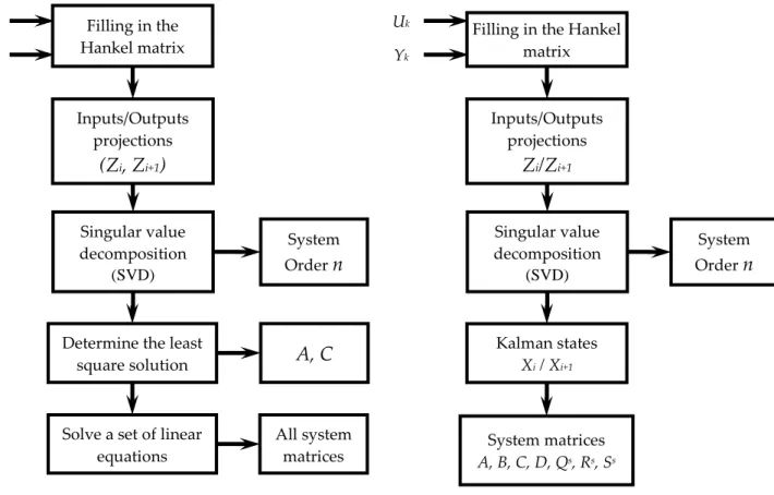
First, the N4SID 1 algorithm is explained in Figure 1. We have therefore, from a finite number of input-output data (𝑈𝑈𝑘𝑘, 𝑌𝑌𝑘𝑘), the possibility to form the Hankel matrices (defined in appendix A)�𝑌𝑌𝑝𝑝, 𝑌𝑌𝑓𝑓�𝑇𝑇 and �𝑈𝑈𝑝𝑝, 𝑈𝑈𝑓𝑓�𝑇𝑇 . In addition, we deduce the oblique projections (𝑍𝑍𝑖𝑖, 𝑍𝑍𝑖𝑖−1).
Figure 1. Steps of the N4SID1 algorithm.
Figure 2. Steps of the N4SID2 algorithm. Filling in the Hankel matrix Inputs/Outputs projections
(Z
i, Z
i+1)
Singular value decomposition (SVD) System Ordern
Determine the least
square solution
A, C
Solve a set of linear
equations All system matrices Uk
Yk
Filling in the Hankel matrix Inputs/Outputs projections
Z
i/Z
i+1 Singular value decomposition (SVD) System Ordern
Kalman states Xi / Xi+1 System matrices A, B, C, D, Qs, Rs, Ss Uk YkThese projections are useful in determining the combined system. Indeed, the linear combinations to be made from the input-output block Hankel matrices to generate (𝑍𝑍𝑖𝑖, 𝑍𝑍𝑖𝑖−1) (projections defined in the appendix C) are functions of the system matrices. Moreover, the system matrices can be retrieved from these linear combinations, as shown in the appendix C.
From input-output we can define the extended observability matrix 𝛤𝛤𝑖𝑖. Trough 𝛤𝛤𝑖𝑖= [𝐶𝐶 𝐶𝐶𝐴𝐴 … . 𝐶𝐶𝐴𝐴𝑖𝑖−1] , we are able find the A and C matrices:
• Matrix C: If we show the extended observability matrix, it is important to note that we can extract directly from the first row of 𝛤𝛤 the C matrix.
• Matrix A: It is determined from the shift structure of 𝛤𝛤𝑖𝑖, denoting : 𝛤𝛤𝑖𝑖= 𝛤𝛤𝑖𝑖𝐴𝐴 ; where 𝛤𝛤𝑖𝑖 is the matrix 𝛤𝛤𝑖𝑖 without the last l rows: 𝛤𝛤𝑖𝑖= (𝐶𝐶 𝐶𝐶𝐴𝐴 … 𝐶𝐶𝐴𝐴𝑖𝑖−2). 𝛤𝛤𝑖𝑖 is without the first l rows: 𝛤𝛤𝑖𝑖= (𝐶𝐶𝐴𝐴 𝐶𝐶𝐴𝐴2 … 𝐶𝐶𝐴𝐴𝑖𝑖−1). Therefore, the matrix A is expressed as: 𝐴𝐴 = 𝛤𝛤𝑖𝑖+𝛤𝛤𝑖𝑖. Later then, we de-termine the rest of system matrices B, D, Qs, Rs and Ss from linear regression algorithm and
the resolution of linear combination demonstrated in appendix C.
This means N4SID 2 does not need to go through the complicated step 4 shown in Figure 1. However, it is clearly explained in the appendix C for determining B and D matrices as shown in Figure 2. Also, the Kalman states are determined as it is explained in (Verhaegen, 1994).
7. Multiple model control
A multiple model or T-S (Takagi-Sugeno) model is a nonlinear system in the form of linear inter-polation of n premises. The three methods used for obtaining the multiple model representation are: 1) the identification technique, 2) linearization around different operating points, and 3) polytopic trans-formation. In the first step, we identify the model parameters based on the given input-output. The second and third steps are assumed to have a nonlinear mathematical model.
Conditions on stability and stabilization of discrete-Time T-S (Takagi-Sugeno) systems will be shown in the next section. Stability analysis is derived via quadratic Lyapunov function method and LMIs (Linear Matrix inequalities) formulation, obtained from BMIs (Bilinear Matrix Inequality). Dis-crete-Time T-S systems using improved PDC (Parallel Distributed Compensation) technique was ap-plied in order to estimate state with the multi-observer technique..
We considered a Takagi-Sugeno (T-S) model described by fuzzy IF-THEN rules. The ith rule of the model is of the following form:
Rule i
𝐼𝐼𝐼𝐼 𝐼𝐼1(𝑘𝑘) 𝑖𝑖𝑖𝑖 𝑀𝑀1𝑖𝑖 𝑎𝑎𝑎𝑎𝑎𝑎 … 𝐼𝐼𝑛𝑛(𝑘𝑘)𝑖𝑖𝑖𝑖 𝑀𝑀𝑛𝑛𝑖𝑖 𝑇𝑇𝑇𝑇𝑇𝑇𝑇𝑇 �𝑥𝑥(𝑘𝑘 + 1) = 𝐴𝐴𝑦𝑦(𝑘𝑘) = 𝐶𝐶𝑥𝑥(𝑘𝑘)𝑖𝑖𝑥𝑥(𝑘𝑘) + 𝐵𝐵𝑖𝑖𝑢𝑢(𝑘𝑘),
where 𝑀𝑀1i, … . 𝑀𝑀𝑛𝑛𝑖𝑖 are the fuzzy sets and n is the number of the rules. In addition, 𝑥𝑥𝑘𝑘∈ ℝ𝑛𝑛 is the state vector; 𝑢𝑢𝑘𝑘 ∈ ℝ𝑝𝑝 is the measurable output vector; 𝐴𝐴𝑖𝑖, 𝐵𝐵𝑖𝑖 and 𝐶𝐶 are the system matrices with appro-priate dimension. Then, the premise variables are 𝑍𝑍(𝑘𝑘) = [𝑍𝑍1(𝑘𝑘) … . 𝑍𝑍𝑞𝑞(𝑘𝑘)] .Therefore, a T-S model is based on the interpolation between several LTI local models using the following equations:
x(k + 1) = ∑ μni=1 i�Z(k)��Aix(k) + Biu(k)� and (8) �∑ μni=1 i�Z(k)� = 1 μi(Z(k)) ≥ 0 with, (9) μi(Z) =∑ wwi(Z(t)) i(Z(t)) n i=1 ; wi�Z(t)� = � Mji(Z(t)) q j=1 .
The approach proposed in this research project is based on the quadratic Lyapunov function. Choosing a Lyapunov function that guarantee stability in simple terms requires a symmetric matrix which is positively defined. Practically, it is simple to implement using 𝑉𝑉(𝑥𝑥(𝑘𝑘)) such as:
V�x(k)� = XkTPXk. (10)
The Discrete T-S fuzzy system is asymptotically stable. If a common matrix 𝑃𝑃 = 𝑃𝑃𝑇𝑇 > 0 exists, then the following LMI is feasible (Boyd et al., 1994, Tanaka et al., 1998):
�A P > 0 . i
TPA
i− P < 0. (11)
7.2 Stabilization of a discret multiple state feedback
The stabilization technique used in this paper is the Parallel Distributed Control (PDC) law, which is written as follow:
u(k) = − ∑ μni=1 i(Z(k))Kix(k). (12) Using the discrete multiple models previously described in (8), a closed loop control law by PDC is given by:
�x(k + 1) = ∑ ∑ μni=1δ nj=1 i�Z(k)�μj�Z(k)�δijx(k).
Hypothesis: The two matrices (𝐴𝐴𝑖𝑖, 𝐵𝐵𝑖𝑖) are assumed to be controllable. It is said that the multiple models is locally controllable as described in (Euntai and Heejin, 2000).
The stabilization conditions for discrete-time multiple models using closed-loop PDC control law require a symmetric matrix 𝑃𝑃 > 0 and matrices 𝐾𝐾𝑖𝑖, ∀𝑖𝑖 ∈ 𝐼𝐼𝑛𝑛 such as:
� ld(δii, P) < 0, ∀i ∈ In, ld�δij, P� ≤ 0, ∀i, j ∈ In2 μi(Z(k))μj(Z(k)) ≠ 0. and, (14) ld�δij, P� = �δij+δ2 ji� T P �δij+δji 2 � − P, with (15) δij= Ai− BiKj. The following conditions are:
(Ai− BiKi)TP(Ai− BiKi) − P < 0. (16) In pre and post multiplying by 𝑃𝑃−1, we obtain:
P−1(A
iP−1− BiKiP−1)TP(AiP−1− BiKiP−1) > 0. (17) It’s assumed that 𝑋𝑋 = 𝑃𝑃−1 and 𝑇𝑇
𝑖𝑖= 𝐾𝐾𝑖𝑖𝑃𝑃−1 ; then we obtain:
X(AiX − BiKiX)TP(AiX − BiNi) > 0. (18) Using the Schur complement, the above condition is written in the form of LMI:
�A X ∗
iX − BiNi X� > 0 ∀ 𝑖𝑖 ∈ 𝐼𝐼𝑛𝑛. (19) By using the same method, the condition 𝑙𝑙𝑑𝑑�𝛿𝛿𝑖𝑖𝑖𝑖, 𝑃𝑃� ≤ 0 is written as:
�Ai+Aj X ∗
2 X − 1
2(BjNi+ BiNj) X� ≥ 0 ∀(𝑖𝑖, 𝑗𝑗) ∈ 𝐼𝐼𝑛𝑛
2, 𝑖𝑖 < 𝑗𝑗. (20)
Now the discrete multiple models in (8) is globally asymptotically stable via improved PDC con-trol law, especially if there are symmetric matrices such as 𝑃𝑃 = 𝑃𝑃𝑇𝑇 > 0 and 𝑄𝑄 = 𝑄𝑄𝑇𝑇 ≥ 0 which verifies (Chadli et al., 2002): � ld(δii, P) + (r − 1)Q < 0, ∀i ∈ In, ld�δij, P� − Q ≤ 0, ∀i, j ∈ In2, i < j, μi(Z(k))μj(Z(k)) ≠ 0. (21) ld�δij, P� = �δij+δ2 ji� T P �δij+δji 2 � − P. (22)
By using matrices 𝑄𝑄𝑖𝑖𝑖𝑖,
𝑄𝑄
𝑖𝑖𝑖𝑖, due to the conservatism and pessimism results, we can define thefol-lowing theorem presented in (Euntai and Heejin, 2000). Theorem: if matrices 𝑃𝑃 = 𝑃𝑃𝑇𝑇 > 0, 𝑄𝑄
𝑖𝑖𝑖𝑖 = 𝑄𝑄𝑖𝑖𝑖𝑖𝑇𝑇 and matrices 𝐾𝐾𝑖𝑖 exists, which verify the equation below:
� ld(δii, P) + (r − 1)Q < 0, ∀i ∈ In. ld�δij, P� − Q ≤ 0, ∀i, j ∈ In2, i < j μi(Z(k))μj(Z(k)) ≠ 0. . (23) Q = �Q11… . Q1n Q1n… . Qnn�. (24)
Then the multiple models in (8) is globally asymptotically stable. Thus, the BMIs of the previous theorem can be transformed into LMIs, which gives:
⎩ ⎨ ⎧ X = PY −1. ii= XQijX. Ki = NiX−1. ∀i ∈ In. (25) 8. Synthesis of multi-observers
Synthesis techniques based on state feedback (PDC control law) need to have the entire state vector 𝑥𝑥(𝑘𝑘), as shown in equations (12)-(13). Therefore, we need to rebuild the state based system using the following multiobservers:
�x�(k + 1) = μi�Z(k)��Aix�(k) + Biu(k)� + Li�y(k) − y�(k)�.
y�(k) = ∑ μni=1 i�Z(k)�Cix�(k). (26)
Knowing that the estimation of the state vector error is given by:
x�(k) = x(k) − x�(k). (27)
The dynamics of the estimation error could then be written as: �x�(k + 1) = ∑ ∑ μni=1 nj=1 i�Z(k)�μj�Z(k)�θijx�(k).
θij= Ai− LiCj , ∀(i, j) ∈ In2. . (28) The synthesis of a multiple observer is used in determining local gains 𝐿𝐿𝑖𝑖∈ 𝐼𝐼𝑛𝑛 to ensure the con-vergence to zero of the dynamics of the estimation error. We have to ensure that there is 𝑃𝑃 = 𝑃𝑃𝑇𝑇 > 0 and matrices 𝐿𝐿𝑖𝑖∈ 𝐼𝐼𝑛𝑛 that verify:
� ld(θii, P) < 0, ∀i ∈ In. ld�θij, P� ≤ 0, ∀i, j ∈ In2 μi(Z(k))μj(Z(k)) ≠ 0. . (29) ld�θij, P� = �θij+θ2 ji� T P �θij+θji 2 � − P. (30)
Then the estimation error converges to zero. The conditions of the previous theorem can be transformed into LMIs using the Schur complement:
�P Ai+Aj P ∗ 2 − 1 2�NjCj+ NjCi� P� ≥ 0. (31) ∀(i, j) ∈ In2 , i < j. (32)
The previous multiple observers may be improved by the following theorem. The multiple ob-servers is globally asymptotically stable if there exist a symmetric matrices 𝑃𝑃 > 0 , 𝑄𝑄𝑖𝑖𝑖𝑖 and 𝐿𝐿𝑖𝑖∈ 𝐼𝐼𝑛𝑛 that satisfy: ⎩ ⎪ ⎪ ⎨ ⎪ ⎪ ⎧ld(θii, P) + Qii< 0, ∀i ∈ In. ld�θij, P� + Qij≤ 0, ∀i, j ∈ In2. �Q11 Q1n Q1n Qnn� . μi�z(k)�μj�z(k)� ≠ 0. θij= Ai− LiCj∀(i, j) ∈ In2. (33)
The matrix inequalities are written as:
⎩ ⎪ ⎪ ⎪ ⎨ ⎪ ⎪ ⎪ ⎧ P > 0. � P − QPA ii ∗ i− NiCi P� > 0 ∀ i ∈ In. �PAi+Aj P − Qij ∗ 2 − 1 2(NiCj+ NjCi) P � ≥ 0 ∀ i, j ∈ In2, i < j Q = �QQ11… . Q1n 1n… . Qnn� . Ni= PLi. . (34) 9. Numerical example
In this section, we apply our theoretical development to confirm and explain our contribution with a numerical example.
9.1. System identification using N4SID1 and 2
Here, we considered the following described by the state matrix A, input vector B, output matrix C, and the direct transmission matrix D.
These matrices are in continuous time and, however, we must discretize them so they can be us-able in our algorithms. For this purpose, the following N4SID representation was considered:
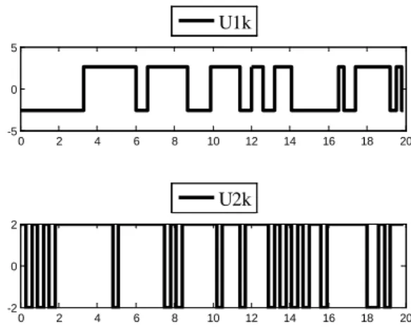
𝑥𝑥𝑘𝑘+1 = 𝐴𝐴𝑥𝑥𝑘𝑘+ 𝐵𝐵𝑢𝑢𝑘𝑘+ 𝑤𝑤𝑘𝑘. (35) 𝑦𝑦𝑘𝑘 = 𝐶𝐶𝑥𝑥𝑘𝑘+ 𝐷𝐷𝑢𝑢𝑘𝑘+ 𝑣𝑣𝑘𝑘. (36) We will identify a multivariable system, which has two inputs and two outputs. First, we will show the estimation results of N4SID1 and then N4SID2. The identification results are obtained for a sampling time Te =0.1 second. In addition, we used the pseudo-random binary signal (PRBS), shown in Figure 4, in order to add noise in the data and demonstrate algorithm robustness.
Figure 3. Real continuous system step response.
The studied system is a multiple-input / multiple-output (MIMO) system, as the inputs are u1 and u2 and the outputs are y1 and y2. We excite the system by an input step and we have then, as shown in Figure 3, different combinations of inputs / outputs. Thereafter, we simulated using Matlab environment the tracing of Bode magnitude plot associated to the MIMO system, which is described by a state representation formed by the A, B, C, and D matrix.
Figure 4. Generation of two PRBS for identification of 2 input system.
A pseudo-random binary sequence "PRBS" is an exciter signal that correctly identifies the pa-rameters of a dynamic model like a black box model. Figure 4 shows the two PRBS used for the system identification. The first PRBS have a [2.6, -2.6] amplitude called U1k, while the second PRBS signal have a [2. 2] amplitude called U2k. The binary pseudorandom sequence is shown between samples [1, 200], knowing that the sampling time is equal to 0.1. The PRBS is a train of amplitude niche (variants between two terminals) that is approached from a discrete white noise rich in frequency.
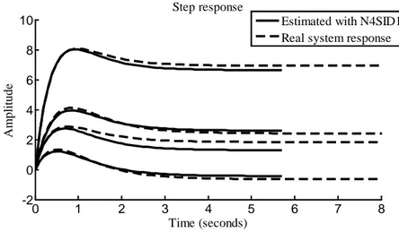
Figure 6 represents the frequency responses, where we note a similarity between the results with different combinations of inputs / outputs which confirm the identification effectiveness of N4SID al-gorithm. Therefore, Figure 6 shows the comparison between the real discretized system and N4SID 2 algorithms. 0 2 4 6 8 10 -2 0 2 4 6 8 10 Time (seconds) A mp litu d e Step response
Real system response
0 2 4 6 8 10 12 14 16 18 20 -5 0 5 U1k 0 2 4 6 8 10 12 14 16 18 20 -2 0 2 U2k
Figure 5. Step response using N4SID2. 0 2 4 6 8 10 -2 0 2 4 6 8 10 Time (seconds) A mp litu d e Step response
Estimated with N4SID 2 Real system response
Figure 6. Frequency response using N4SID2 algorithm. -10 0 10 M agni tude ( dB ) 10-2 10-1 101 -90 0 90 180 270 360 450 P has e ( deg) Frequency (rad/s)
Estimated with N4SID2 Real system response
0 10 20 M agni tude ( dB ) 10-1 101 -180 -135 -90 -45 0 45 P has e ( deg) Frequency (rad/s)
Estimated with N4SID2 Real system response
-10 0 10 M agni tude ( dB ) 10-2 10-1 101 -900 90 180 270 360 450 540 P has e ( deg) Frequency (rad/s)
Estimated with N4SID2 Real system response
-10 0 10 20 M agni tude ( dB ) 10-2 10-1 101 -180 -90 0 90 P has e ( deg) Frequency (rad/s)
Estimated with N4SID2 Real system response
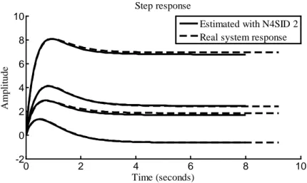
Figure 7. Step response using N4SID1 algorithm.
Figure 7 represents the step responses of the discretised real system and the identified system with N4SID 1. They are presented respectively by the black continued line and the black discontinuous line. Computation time is an important parameter for industrial process. Therefore, Table 1 compare the identification time for the MIMO system. Also, Table 2 shows the mean squared error (MSE) be-tween the estimated models by both N4SID algorithms and MOESP algorithm. The lowest value indi-cates the best algorithm which is N4SID2.
Table 1. Algorithm computation time for identification of one MIMO system.
N4SID 1 N4SID 2 MOESP
0.2969 0.5625 0.6250
Table 2. MSE in time domain for both N4SID and MOESP algorithms compared to the real system.
N4SID 1 N4SID 2 MOESP
2.4940 0.5625 0.6250 0 1 2 3 4 5 6 7 8 -2 0 2 4 6 8 10 Time (seconds) A mp litu d e Step response
Estimated with N4SID1 Real system response
Figure 8. Frequency response comparing N4SID1
response and real system response.
Figure 9. Frequency response comparing MOESP response and real system response.
-10 0 10 M agni tude ( dB ) 10-2 10-1 101 -90 0 90 180 270 360 450 P has e ( deg) Frequency (rad/s)
Estimated with N4SID1 Real system response
0 10 20 M agni tude ( dB ) 10-1 101 -180 -135 -90 -45 0 45 P has e ( deg) Frequency (rad/s)
Estimated with N4SID1 Real system response
-10 0 10 M agni tude ( dB ) 10-2 10-1 101 -90 180 540 P has e ( deg) Frequency (rad/s)
Estimated with N4SID1 Real system response
-10 0 10 20 M agni tude ( dB ) 10-2 10-1 101 -180 -90 0 90 P has e ( deg) Frequency (rad/s)
Estimated with N4SID1 Real system response
-10 0 10 M agni tude ( dB ) 10-2 10-1 101 -90 0 90 180 270 360 450 P has e ( deg) Frequency (rad/s)
Estimated with MOESP Real system response
0 10 20 M agni tude ( dB ) 10-2 10-1 101 -180 -135 -90 -45 0 45 P has e ( deg) Frequency (rad/s)
Estimated with MOESP Real system response
-10 0 10 M agni tude ( dB ) 10-3 10-2 101 -900 90 180 270 360 450 540 P has e ( deg) Frequency (rad/s)
Estimated with MOESP Real system response
-20 0 20 M agni tude ( dB ) 10-3 10-2 101 -180 -90 0 90 P has e ( deg) Frequency (rad/s)
Estimated with MOESP Real system response
Figure 10. Zoom on first results of samples [1,200] using N4SID1 and N4SID2.
Figure 10 represents the comparison between the outputs of the discretised real model and the identified outputs model. It makes comparisons between the simulations of the obtained model with measured data, in order to validate a model.
0 2 4 6 8 10 12 14 16 18 20 -30 -20 -10 0 10 20 30 40
Output y1 of the real system Estimated output y1 with N4SID 1
0 5 10 15 20 -30 -20 -10 0 10 20 30 40
Output y1 of the real system Estimated output y1 with N4SID 2
0 2 4 6 8 10 12 14 16 18 20 -20 -15 -10 -5 0 5 10 15 20
Figure 11. Zoom on second output results of samples [1,200] using N4SID1 and N4SID2.
Figure 11 represents the comparison between the outputs y2 of the discretized real model and the output y2 of the estimated models with the two identification algorithms N4SID 1 and N4SID 2. 9.2. Multiple model stabilization
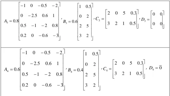
In this part of the article, we are interested in stabilization of the multiple models. In the previ-ous section, we studied only one model with two inputs and two outputs. In this section, we study the stability and stabilization of four MIMO models (each model are LTI with two inputs and two out-puts). The T-S is formed by the matrices identified by N4SID2 since the results are more accurate than N4SID1 and MOESP using MSE criterion (see Table 2). The states matrices Ai, represented in equation (8), that represent the multiple models, the input vectors, and the output vectors of each local linear model are given as:
− − − − − − − − = 3 6 . 0 0 2 . 0 8 . 0 2 1 5 . 0 1 6 . 0 5 . 2 0 2 5 . 0 0 1 1 A , = 2 3 5 2 2 0 5 . 0 1 1 B , = 5 . 0 1 2 3 3 . 0 5 0 2 1 C , = 0 0 0 0 1 D
−
−
−
−
−
−
−
−
=
3
6
.
0
0
2
.
0
8
.
0
2
1
5
.
0
1
6
.
0
5
.
2
0
2
5
.
0
0
1
85
.
0
2A
, = 2 3 5 2 2 0 5 . 0 1 63 . 0 2 B , = 5 . 0 1 2 3 3 . 0 5 0 2 2 CD
2=
0
0 5 10 15 20 -15 -10 -5 0 5 10 15 − − − − − − − − = 3 6 . 0 0 2 . 0 8 . 0 2 1 5 . 0 1 6 . 0 5 . 2 0 2 5 . 0 0 1 8 . 0 3 A , = 2 3 5 2 2 0 5 . 0 1 6 . 0 3 B , = 5 . 0 1 2 3 3 . 0 5 0 2 3 C , = 0 0 0 0 3 D
−
−
−
−
−
−
−
−
=
3
6
.
0
0
2
.
0
8
.
0
2
1
5
.
0
1
6
.
0
5
.
2
0
2
5
.
0
0
1
6
.
0
4A
, = 2 3 5 2 2 0 5 . 0 1 4 . 0 4 B , = 5 . 0 1 2 3 3 . 0 5 0 2 4 C , D4=0From (26) and (34), the feedback gain 𝐾𝐾𝑖𝑖, the matrix 𝑃𝑃 , and the gain 𝐿𝐿𝑖𝑖 matrix can be obtained as: 1
.
.
.
i i i iP
X
K
N P
N
PL
− =
=
=
(37)Solving LMIs system using (34) and (37), we obtain:
=
0.6214
0.0465
0.0324
0.0867
0.0465
0.1888
0.0300
0.0320
0.0324
0.0300
0.1409
0.1033
-0.0867
0.0320
0.1033
0.6384
P
,
=
1.1506
0.0100
0.1941
0.3941
2.2542
0.2190
0.3336
0.1654
-1
K
,
=
0.7680
0.1422
0.0491
0.5701
-1.5345
0.0541
0.2250
0.1609
-2
K
,
=
0.8109
0.0513
0.0446
0.5965
-1.6386
0.1572
0.2276
0.1374
-3
K
,
=
1.0189
0.1185
0.1578
0.7914
2.0304
0.1928
0.4688
0.1687
4
K
,
=
0.2075
0.1673
0.2630
0.1902
-1.5255
0.6019
0.6126
0.2415
-1
L
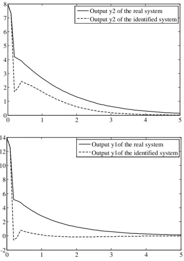
, = 0.5000 0.3345 0.6706 0.3946 -2.9498 1.2732 0.4415 0.4337 -2 L , = 0.4825 0.3256 0.6031 0.3425 -3.1157 1.3848 0.5576 0.3757 -3 L , = 0.1060 0.1315 0.2843 0.2834 -1.6519 0.7727 0.4968 0.5692 -4 L .Figure 12 shows respectively the output y1(t) and y2(t) of the multivariable fuzzy system with real and identified parameters. The system is globally asymptotically stable because we observed that y1(t) and y2(t) converge towards zero.
Figure 12. Output y1, y2 of the real and identified system stabilized with the improved PDC
control law.
However, these results present the stabilization of the multiple model system. The real system and the identified one described by Figure 12 were observed as a global asymptotic stabilization. The stabilization of the identified multiple model built it by the estimated matrices through N4SID 2 algo-rithm. We observe also that all trajectories of the above fuzzy system converge to zero.
10. Conclusion
In this paper, we used two N4SID algorithms for the identification of multivariable systems and we compare our proposed algorithm with the MOESP. The N4SID algorithms subspace identification methods differ from other classic identification algorithms in their concept, interpretation, and compu-tational implementation. We demonstrate the efficiency of an improved N4SID algorithm. In the sec-ond section of this paper, we used the LTI identified model with N4SID2 to build the T-S nonlinear system. After that, we studied various conditions for the global asymptotic stability system. This ap-proach ensures the global asymptotic stability of the closed loop T-S fuzzy systems. Therefore, the sta-bilization results require the quadratic Lyapunov function and all components of the state vector. For this reason, we constructed a multiobserver to estimate the state vector.
0 1 2 3 4 5 0 1 2 3 4 5 6 7 8
Output y2 of the real system Output y2 of the identified system
0 1 2 3 4 5 -2 0 2 4 6 8 10 12 14
Output y1of the real system Output y1of the identified system
11. Acknowledgments
This work is supported financially by the Natural Sciences and Engineering Research Council of Canada (NSERC) under the grant number EGP 477206 – 14, held by Martin Otis.
Appendix A: Mathematical tools
In this appendix, we present the mathematical tools of linear algebra used in subspace method. We define first the extended observability matrix (we extend the observability to an order that is supe-rior to the one of the system) (Van Overschee and De Moor, 1994):
1
.
i iC
CA
CA
−
Γ =
Then, the reversed extended controllability matrix is:
(
1 2)
...
.
i i iA B
A B
B
− −∆ =
The input block Hankel matrix is defined as:
0 1 2 1 2 3 0 1 1 1 2
.
j i j i i i i i ju
u
u
u
u
u
u
u
U
u
u
u
u
− − − + + −
=
,
and the output block Hankel matrix is:
0 1 2 1 2 3 0 1 1 1 2
.
j i j i i i i i jy
y
y
y
y
y
y
y
Y
y
y
y
y
− − − + + −
=
The following matrices are used:
𝑈𝑈
𝑝𝑝= 𝑈𝑈
0|𝑖𝑖−1,
𝑈𝑈
𝑓𝑓= 𝑈𝑈
𝑖𝑖|2𝑖𝑖−1,
𝑈𝑈
𝑝𝑝+= 𝑈𝑈
0|𝑖𝑖and
𝑈𝑈
𝑓𝑓−=
𝑈𝑈
𝑖𝑖+1|2𝑖𝑖−1.
A similar definitions is presented for Hankel block output matrices:𝑌𝑌
𝑝𝑝,
𝑌𝑌
𝑝𝑝+,
𝑌𝑌
𝑓𝑓and,
𝑌𝑌
𝑓𝑓+where subscript stands ‘f’ for the “future” and ‘P’ for the “past”.For the stochastic sub- model (6)-(7), we define:
( )
( )
( )
+ = = Λ + = = ∇ + = = + + . . . 1 0 1 s T s T s k s k s T s T s k s k s T s T s k s k s R C CP y x E S C AP y x E Q A AP x x E P(
1)
... . s i i A A − ∆ = ∇ ∇ ∇The Block lower triangular Toeplitz matrix and the block Toeplitz cross covariance matrix are:
2 3 4
0
0
0
0
0
.
0
d i i i iD
CB
D
D
H
CAB
CB
CA
−B
CA
−B
CA
−B
D
=
and 2 3 40
0
0
0
0
.
0
s i i i iI
CK
I
I
H
CAK
CK
CA
−K
CA K
−CA
−K
K
=
Appendix B: Kalman states
From the matrices of block Hankel, the matrices system are determined directly through the de-termination of projections from which to estimate the two states sequences which are the outputs of the extended Kalman filter (Van Overschee and De Moor, 1994):
].
[
].
[
1 1 s j i s i s i d j i d i d ix
x
X
x
x
X
− + − +=
=
If both noises are jointly Gaussian, we have the best estimates of the Kalman states in the quad-ratic mean sense. If we knew the initial states 𝑋𝑋�0 and its covariance 𝑃𝑃0 , inputs and outputs
𝑢𝑢 =
[𝑢𝑢
1𝑢𝑢
2⋯ 𝑢𝑢
𝑛𝑛], 𝑦𝑦 = [𝑦𝑦
1𝑦𝑦
2⋯ 𝑦𝑦
𝑛𝑛]
and all system matricesA
,
B
,
C
,
D
,
Q
,
S
,
R
,
the states can be easilycomputed using the following recursive formulas:
(
)
(
)(
) (
)
(
)(
) (
)
∇
+
+
Λ
∇
+
−
=
∇
+
+
Λ
∇
+
=
−
−
+
+
=
− − − − − − − − − − − − − − − −.
.
.
ˆ
ˆ
ˆ
1 1 1 0 1 1 1 1 1 0 1 1 1 1 1 1 1 1 T T k T k T k T k k T T k T k T k k k k k k k k kC
AP
C
CP
C
AP
A
AP
P
C
AP
C
CP
C
AP
K
Du
x
C
y
K
Bu
x
A
x
Based on last equation, we computed the Kalman gain and recursively defined the error covari-ance matrix
E
[
(
x
k−
x
ˆ
k)(
x
k−
x
ˆ
k)
T]
which estimatess
P
.
From previous equations, it was possible to establish the following formulas:
(
ˆ
)
.
ˆ
ˆ
1 i ii i ii i ii iA
X
BU
K
Y
C
X
DU
X
+=
+
+
−
−
(
ˆ
)
.
ˆ
i i i i i i i i i iC
X
BU
Y
C
X
DU
Y
=
+
+
−
−
If it was possible to obtain Kalman states directly from input- output data, the equations above would satisfy the assumption on consistent applications of least squares to estimate system matrices
D
C
B
A
,
,
,
.
We determine from the residuals matrices the covariance matrices(𝑄𝑄
𝑠𝑠, 𝑆𝑆
𝑠𝑠, 𝑅𝑅
𝑠𝑠) .
Appendix C: Orthogonal projection
In this appendix, we present the geometric tools of linear algebra used in subspace method. We assume that the matrices
A
,
B
,
C
are given.The orthogonal projection of the row space of 𝐴𝐴 into the row space of 𝐵𝐵 is defined as (Van Overschee and De Moor, 1994):
.
)
(
/
B
A
A
B
B
B
B
A
=
Π
B=
t +Where
( )
.
+denotes the Moore-Penrose of the matrix( )
. andΠ
B=
B
T(
B
.
B
T)
+.
B
.
It is im-portant to note thatΠ
𝐵𝐵 defined the operator of orthogonal projection that projects the row space of matrix onto the row space of the matrix B.The projection of the row space of 𝐴𝐴 into the orthogonal complement of the rowspace of 𝐵𝐵 is:
(
j B)
BA
A
B
A
I
A
B
A
=
Π
⊥=
−
=
−
Π
⊥/
/
,
Where
B
⊥denotes a base of the orthogonal space to the row space of𝐵𝐵
, andΠ
⊥B defines the geometric operator that projects the row space of a matrix onto the orthogonal complement to the row space of the matrix B. From the expression of
Π
𝐵𝐵 andΠ
B⊥,
one can easily show that matrix𝐴𝐴
can bedecomposed into two matrices where their row spaces are orthogonal such as:
A
=
A
Π
B+
A
Π
B⊥.
Therefore, one defines the oblique projection of a matrix 𝐴𝐴 along the row space of the matrix 𝐵𝐵 onto the row space of the matrix :
[
A
B
][
C
B
]
C
A
(
C
)
C
C
A
/
B=
/
⊥.
/
⊥ +.
=
Π
B⊥+
Π
B⊥ +.
Then, another one defines the properties of the orthogonal and oblique projections as follow:
.
0
/
x⊥=
xA
A
.
0
/
x x=
xA
C
A
N4sid method 1The identification algorithm N4SID is determined by four steps which include: Determine the projection
)
.
(
/
1 2 3 1 0 1 2 1 0 1 2
=
=
× × × − − − − p f p li li i mi li i mi li i i i i i i i iY
u
u
L
L
L
Y
u
u
Y
Z
.
1 2 1 1
=
+ − + − + + p f p i i iY
u
u
Y
Z
Computing singular value decomposition (SVD)
Let the matrix M be the rank deficient space which coincides with that of columns Γ𝑖𝑖 . Therefore, we compute the singular value decomposition SVD passing through the following mathematical steps:
.
0
0
0
1 2 1 tV
U
U
M
∑
=
[
]
( )
(
)
[
]
( )
(
)
.
.
.
3 2 1 1 2 1 1 1 i i i mi mi i i i i d i i d i i d i mi i i i i iQ
L
R
S
Q
A
H
L
H
Q
R
S
Q
A
L
Γ
=
Γ
−
Γ
+
=
−
∆
+
Γ
−
Γ
=
+ − − Where (𝑅𝑅−1)1|𝑛𝑛𝑖𝑖 is the sub-matrix of the column 1 to the column mi.
(
)
0
0
.
0
)
(
1 2 1 1 0 1 0 3 1 t i i li li i mi li iU
U
V
Y
u
L
L
∑
=
− − × × 2 1 1 1 1=
Σ
Γ
i−U
where
U
1 denote respectively the lastl
(i−1) rows of U1.
Determine the system matrices
We assume that
Γ
i,
Γ
i−1 and n the order of system are determined.2 1. 1 1 1 1 1 2 1.
ˆ
ˆ
d i i i i i i d i i i i i iZ
X
H U
Z
X
H U
− + − + − + − = Γ
+
= Γ
+
We can extract: 2 1 1 1 1 1 1 2 1.ˆ
(
).
ˆ
(
d i i i i i i d i i i i i iX
Z
H U
X
Z
H U
+ − + + − + − + −
= Γ
−
= Γ
−
In our case, we need to know
H
idand d iH
−1 from: − − − +
+
+
=
i i i i i i iX
u
u
BU
X
A
X
ˆ
ˆ
ˆ
1 0 1 2 0 1 and− − −
+
+
=
i i i i i i i iX
u
u
DU
X
C
Y
ˆ
ˆ
1 0 1 2 0,
Where
( )
.
−indicates a matrix whose row space is perpendicular to the row space of( )
..
Also, we know that:− − +
+
+
=
i i i i i i i i iX
Z
u
U
D
B
X
C
A
Y
X
ˆ
ˆ
ˆ
02 1 1,
Then, if we subtitle the expression for 𝑋𝑋�𝑖𝑖 and 𝑋𝑋�𝑖𝑖+1 , we get: − − − + + + −
+
+
Γ
=
Γ
i i i i i i i i i i iX
Z
U
U
K
K
Z
C
A
Y
Z
ˆ
1 2 0 1 2 22 12 1 1,
where we define:
Γ
−
Γ
Γ
−
Γ
−
Γ
Γ
Γ
−
=
+ − + + − + − − + d i i i i d i i d i i i iH
A
B
D
C
D
H
A
H
B
D
A
B
K
K
0
0
1 1 1 1 22 12.
We observe that the matrices B and D appear linearly in the matrices 𝐾𝐾12 , 𝐾𝐾22. From the last equation, we obtain:
.
/
/
1 2 22 12 1 1Π
Γ
=
Π
Γ
− + + + − i i i i i i i iU
Z
K
C
K
A
Y
Z
The unknown in this set of linear equations are , 𝐶𝐶, 𝐾𝐾12 , 𝐾𝐾22 . The solution is to compute the least mean square: 2 1 2 22 12 1 1 , , , 12 22
min
F i i i i i i i i K K C AU
Z
K
C
K
A
Y
Z
Γ
−
Γ
− + + + − with
+
Γ
×
=
Γ
− + + − + w v i i i i i i i ip
p
U
Z
K
K
K
K
Y
Z
1 2 22 21 12 11 1 1,
where
p ,
vp
ware residues.The system matrix 𝐴𝐴 is equal to 𝐾𝐾11 and 𝐶𝐶 is equal to 𝐾𝐾21 . Then we compute the matrices B and D from 𝐾𝐾12 , 𝐾𝐾22 , 𝐴𝐴 and 𝐶𝐶 by solving a set of linear equations. Finally, we compute the covariance’s matrices as follows:


![Figure 11. Zoom on second output results of samples [1,200] using N4SID1 and N4SID2.](https://thumb-eu.123doks.com/thumbv2/123doknet/7490792.224452/19.892.260.688.117.401/figure-zoom-second-output-results-samples-using-sid.webp)