HAL Id: hal-01485037
https://hal.archives-ouvertes.fr/hal-01485037
Submitted on 8 Mar 2017
HAL is a multi-disciplinary open access
archive for the deposit and dissemination of
sci-entific research documents, whether they are
pub-lished or not. The documents may come from
teaching and research institutions in France or
abroad, or from public or private research centers.
L’archive ouverte pluridisciplinaire HAL, est
destinée au dépôt et à la diffusion de documents
scientifiques de niveau recherche, publiés ou non,
émanant des établissements d’enseignement et de
recherche français ou étrangers, des laboratoires
publics ou privés.
Bayesian sparse estimation of migrating targets for
wideband radar
Stéphanie Bidon, Jean-Yves Tourneret, Laurent Savy, François Le Chevalier
To cite this version:
Stéphanie Bidon, Jean-Yves Tourneret, Laurent Savy, François Le Chevalier. Bayesian sparse
esti-mation of migrating targets for wideband radar. IEEE Transactions on Aerospace and Electronic
Systems, Institute of Electrical and Electronics Engineers, 2014, vol.
50 (n° 2), pp.
871-886.
To link to this article : DOI :
10.1109/TAES.2013.120533
URL :
http://dx.doi.org/10.1109/TAES.2013.120533
To cite this version :
Bidon, Stéphanie and Tourneret, Jean-Yves and Savy,
Laurent and Le Chevalier, François Bayesian sparse estimation of migrating
targets for wideband radar. (2014) IEEE Transactions on Aerospace and
Electronic Systems, vol. 50 (n° 2). pp. 871-886. ISSN 0018-9251
O
pen
A
rchive
T
OULOUSE
A
rchive
O
uverte (
OATAO
)
OATAO is an open access repository that collects the work of Toulouse researchers and
makes it freely available over the web where possible.
This is an author-deposited version published in :
http://oatao.univ-toulouse.fr/
Eprints ID : 17116
Any correspondence concerning this service should be sent to the repository
administrator:
[email protected]
Bayesian Sparse Estimation
of Migrating Targets for
Wideband Radar
ST ´EPHANIE BIDON, Member IEEE
JEAN-YVES TOURNERET, Senior Member IEEE
University of Toulouse France
LAURENT SAVY
ONERA France
FRANC¸ OIS LE CHEVALIER, Senior Member, IEEE
Delft University of Technology The Netherlands
Wideband radar systems are highly resolved in range, which is a desirable feature for mitigating clutter. However, due to a smaller range resolution cell, moving targets are prone to migrate along the range during the coherent processing interval (CPI). This range walk, if ignored, can lead to huge performance degradation in detection. Even if compensated, conventional processing may lead to high sidelobes preventing from a proper detection in case of a multitarget scenario. Turning to a compressed sensing framework, we present a Bayesian algorithm that gives a sparse representation of migrating targets in case of a wideband waveform. Particularly, it is shown that the target signature is the sub-Nyquist version of a virtually well-sampled two-dimensional (2D)-cisoid. A
sparse-promoting prior allows then this cisoid to be reconstructed and represented by a single peak without sidelobes. Performance of the proposed algorithm is finally assessed by numerical simulations on synthetic and semiexperimental data. Results obtained are very encouraging and show that a nonambiguous detection mode may be obtained with a single pulse repetition frequency (PRF).
Authors’ addresses: S. Bidon, Institut Sup´erieur de l’A´eronautique et de l’Espace DEOS, 10 av. E. Belin, 31055 Toulouse cedex 4, FRANCE. E-mail: ([email protected]). J.-Y. Tourneret, IRIT - ENSEEIHT – T´eSA, 2 rue Camichel, BP 7122, 31071 Toulouse cedex 7, FRANCE. L. Savy, ONERA, DEMR, Chemin de la Huni`ere et des Joncherettes, BP 80100 FR-91123 Palaiseau cedex, France. F. Le Chevalier, TU Delft, EEMCS Building, Mekelweg 4, 2628 CD Delft, The Netherlands.
I. INTRODUCTION
Radar systems transmitting a train of pulses at constant pulse repetition frequency (PRF) are subjected to two types of ambiguities: range ambiguities when the PRF is too large to ensure that all echoes are received within the pulse repetition interval (PRI), and velocity ambiguities when the PRF is less than the Doppler spectrum width of the echoes [1]. The unambiguous range Raand velocity va
are linked by the fundamental relation Rava= cλc/4
with c the speed of light and λcthe radar wavelength. It
shows that one cannot increase the ambiguous range without decreasing the ambiguous velocity, and
reciprocally, one cannot increase the ambiguous velocity without decreasing the ambiguous range. Therefore, in many radar applications, range and velocity of a target cannot be retrieved simultaneously without ambiguities [2]. In other words, when choosing the PRF, it is often not possible to comply with the Nyquist sampling criterion to measure both range and velocity of a target.
Radar designers have used different techniques to remove ambiguities and then reconstruct the observed scenario unambiguously. Most of them consist in transmitting several bursts with different PRFs and remove ambiguities via an implementation of the Chinese remainder theorem, e.g., [3]. Nevertheless, these methods entail several drawbacks.
On the other hand, wideband radar systems may offer an alternative and elegant solution to the problem of ambiguity removal [4]. Indeed, let us assume from now on that a low PRF (i.e., there are no range ambiguities but many velocity ambiguities occur) with a wide
instantaneous bandwidth is considered. Due to the subsequent high range resolution, fast moving targets are prone to migrate during the coherent processing interval (CPI) leading to a range-velocity coupling. The received digitized signal can then be seen as a set of coherent observations in adjacent narrowband channels whose analog counterparts would be identical but whose (slow-time) sampling period would increase with the subband [5, 6]. Since a low PRF is under consideration, this means that on each subband the same signal is observed but with a linearly increasing aliasing
phenomenon. From these undersampled observations, one may wonder if the signal can be reconstructed
unambiguously. Hence, the problem of target detection in case of a constant low PRF wideband waveform arises naturally as a compressed sensing problem.1
Compressed sensing or compressive sampling (CS) is a recently new signal processing paradigm that states that
1We stress out here that we do not discuss in this paper the problem of
sampling rate in the fast-time. This is also of great concern since for wideband waveform the number of samples in this dimension may be very high. Nonetheless, this work is concerned only with the problem arising when the slow-time domain is undersampled.
a sparse signal can be fully reconstructed from sub-Nysquist observations [7, 8]. It is generally a two-part problem where on one hand the undersampling scheme is studied and on the other hand reconstruction algorithms are designed to fully recover the low-rate observed signal. CS constitutes thus a genuine
breakthrough and has been investigated in many domains of application; radar is obviously one of them [9–14]. In the case of our low PRF wideband signal, the observed data are naturally undersampled so that one is left here with the unambiguous reconstruction of the observed scenario. Assuming compressibility of the signals of interest (i.e., the targets), the reconstruction problem appears then as an ill-posed problem. So far, ℓp>0-norm
minimization approaches have been mostly used to estimate the target scene in various radar applications: see [12,15] and references therein. Note also the ℓ1
penalized least squares method applied to wideband signal in [16]. We propose here to regularize the estimation problem via a fully Bayesian approach where not only a sparsity inducing prior is used to describe the signals of interest but also the estimation process is led via a Monte-Carlo Markov chain (MCMC). A Bayesian framework has been favored in this work due to several advantages it has been offering [17]. Firstly, instead of providing only an estimate of the radar scenario, other parameters are also estimated (i.e., thermal noise power, average target power, level of sparsity). Moreover, not only point estimates are obtained but full posterior distributions are estimated which may be of interest to obtain measures of confidence for the estimates. Furthermore, in our case, only a few parameters have to be tuned by the radar operator. As introduced later, these parameters have a direct physical meaning, which renders the tuning comprehensible.
The remainder of the paper is organized as follows. In Section II, the conventional data model for a low PRF wideband signal is presented. Particularly, the signature of interest is interpreted as a bidimensional cisoid whose undersampling increases linearly with the subband. Then in Section III, assuming a clutter-free scenario, a hierarchical Bayesian model is presented where a sparse promoting prior is assumed to favor a sidelobeless representation of the targets. Minimum mean square error (MMSE) and maximum a posteriori (MAP) estimators are derived accordingly. Performance of the Bayesian estimators is then assessed in Sections IV and V via synthetic data and experimental data collected from the PARSAX radar system [18]. Section IV concludes with a discussion on upcoming extensions to this work.
II. SIGNAL MODEL FOR WIDEBAND RADAR In this section, the data model for a wideband radar system is introduced. A particular focus is put on the scatterer signature that is shown to be the undersampled version of a virtual but well-sampled signal.
A. Radar System and Received Signals
The system under consideration is a pulsed-Doppler radar with wideband waveform. The radar sends a series of M pulses with PRF fr= 1/Trwhere Tris the PRI. By
wideband we mean that the bandwidth B is nonnegligible compared with the carrier frequency fc= c/λc.
Furthermore, the range migration of each scatterer is assumed to be negligible within the duration Tpof a single
pulse but may be significant during the whole CPI, viz vTp≪ δR and vMTr≫ δR
where v is the (constant) radial velocity of the scatterer and δR= c/(2B) is the range resolution. A low PRF is
considered so that no-range ambiguities occur but the maximal Doppler frequency is aliased, i.e., 2vmaxfc/c >
1/(2 Tr) where vmaxrepresents the maximum target
velocity expected for a scatterer.
Usually with narrowband radar, detection is performed range gate by range gate. Nevertheless, in case of a wideband waveform, moving targets migrate so that detection is more conveniently performed on low range resolution (LRR) segments consisting of the returns collected on K adjacent range gates [5, 19, 20]. Samples to be processed can thus be represented by a K × M matrix where the first and second dimensions refer, respectively, to the fast- and slow-time. However, the data model can be more conveniently expressed after applying a range transform (a simple fast Fourier transform (FFT)) on the fast-time. Thus, it is assumed in the following that the samples are expressed in the fast-frequency/slow-time domain.
In absence of clutter and in case of multiple scatterers in the scene, the K × M data matrix can finally be expressed as Y = N X t =1 αtAt+ N (1)
where N is the receiver noise and N, αt,and Atrepresent,
respectively, the number of scatterers, the tth complex amplitude, and signature. The receiver noise is assumed to be spectrally white on both dimensions and is modeled by a white Gaussian random signal with power σ2. The
signature Atis detailed in the next section.
Note that in the remainder of the paper, an equivalent vector notation is also used for (1), i.e.,
y =
N
X
t =1
αtat+ n (2)
where each KM-length vector involved is the row-vectorization of its clearly identifiable matrix counterpart.
B. Scatterer Signature
1) Conventional Expression:The scatterer signature A involved in (1) has been studied earlier in e.g., [5, 19–21] and was shown to be the product of a two-dimensional
(2D) cisoid with cross-coupling terms. More precisely, the (k, m)th element of the matrix A can be expressed by
[ A]k,m= exp ½ j2π µ −τ0 B Kk+ 2vfc c Trm ¶¾ (2D-cisoid) × exp ½ j2π2v c B KTrkm ¾
(cross-coupling terms)
(3) where τ0designates the initial round-trip delay of the
scatterer. The 2D-cisoid in (3) is a conventional term that involves the usual range frequency –τ0and the Doppler
frequency 2v fc/c associated, respectively, with the
sampling periods B/K and Tr. The cross-coupling terms are
specific to the wideband waveform and model the range migration. It is worth noticing that, aside from the system parameters, these terms depend only on the radial velocity
v. More information may therefore be retrieved about the scatterer velocity in the case of a wideband waveform when compared with a narrowband waveform. Moreover, measuring velocity via range migration is unambiguous contrary to Doppler frequency measurement.
A simple and straightforward way to exploit this additional information is to sum coherently the samples of the target signature (3). The resulting estimated amplitude vector is given by [5, 22]
ˆαCI=
aHy
kak22
(4) and can be implemented efficiently via a Keystone-like transform [21, 23]. Unlike a conventional Doppler processing, the coherent integration (4) allows the gain on the target peak to be preserved [24]. However, high sidelobes remain at ambiguous velocities rendering the processing inadequate in case of a multitarget scenario. We propose hereafter a novel interpretation of (3) to more deeply exploit the information brought by the range migration.
2) Towards a Sparse Representation:
a) Interpretation of the scatterer signature: To go one step further with the expression of the scatterer signature, we rewrite the expression (3) as follows
[ A]k,m= exp ½ j2π µ −τ0 B Kk + 2vfc c Tr,km ¶¾ (5) where Tr,k= µ 1 +KfB c k ¶ Tr. (6)
Looking carefully at these two expressions, it appears that for a given subband k, the scatterer signal is a 1D-cisoid with the same Doppler frequency as in (3) but with a subband-dependent sampling period Tr,kwhich
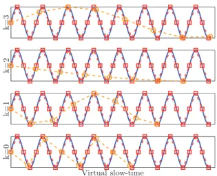
increases linearly with the subband index. As a low PRF has been previously assumed, this means that aliasing on the slow-time occurs and increases with the subband index too. This phenomenon is illustrated in Fig. 1 where a 1D-sine has been represented K times but with a linearly
Fig. 1. Observation and resampling of a cisoid. Solid line represents analog version of cisoid with frequency 2vfc/c. Circle markers represent
observed data with period Tr,k. Square markers represent samples of cisoid obtained with thinner period ¯Trindependent of subband index k.
increasing sampling period (circle markers). As can be observed, the higher the subband index, the slower the observed sine.
b) Shannon reconstruction: According to the Shannon reconstruction theorem [25], each element [ A]k,mcan be
written via the following interpolation formula [ A]k,m= +∞ X ¯ m=−∞ [ ¯A]k,m¯sinc ½ π µ mT¯r,k Tr − ¯ m ¶¾ (7) where ¯Tris a sampling period that complies with the
sampling theorem, i.e., 2vmaxfc
c < 1 2 ¯Tr
(8) and ¯A is the 2D-cisoid with frequency pair (–τ0, 2vfc/c)
and sampling periods (B/K, ¯Tr)
[ A]k,m¯ = exp ½ j 2π µ −τ0 B Kk + 2vfc c T¯rm¯ ¶¾ . (9) For a given subband k, the signal (9) corresponds to the same 1D-cisoid as in (5) but this time with a constant sampling rate ¯fr = 1/ ¯Trchosen large enough to avoid
aliasing. Such samples are represented in Fig. 1 with square markers. Interestingly, the virtual samples [ ¯A]k,m¯ in
(9) correspond to data that would be received by a narrowband radar (no range migration) with virtual sampling period ¯Tr.By defining a new sampling period,
one defines also a new ambiguous velocity ¯va= cf0/(2 ¯fr)
larger than the initial ambiguous velocity va. Thus, if one
had access to samples [ ¯A]k,m¯ and taking into account the
condition (8), one would have a nonambiguous mode. In the remainder of this paper, we are interested in estimating such samples. However, prior to that, it is worth noticing that the formula (7) involves for each subband k an infinite number of samples {[ ¯A]k,m¯}m∈Z¯ .To make the estimation
possible, we use a truncated version of (7), viz [ ¯A]k,m 1 = ¯ M−1 X ¯ m=0 [ ¯A]k,m¯sinc ½ π µ mTr,k¯ Tr − ¯ m ¶¾ (10) with ¯Mthe number of virtual pulses considered. It is chosen to ensure that for each subband, (10) is actually an interpolation and not an extrapolation formula, namely
¯ M ≥ » M µ 1 + fB c K − 1 K ¶ Tr ¯ Tr ¼ (11) where ⌈·⌉ denotes the operator that rounds towards plus infinity. Note that ¯Mcould be chosen as a
subband-dependent parameter. However, for the sake of simplicity this route is not taken here.
Applying the truncated-interpolation formula (10) to each scatterer involved in the received signal (1) yields
[Y ]k,m= ¯ M−1 X ¯ m=0 [ ¯3]k,m¯sinc ½ π µ mTr,k¯ Tr − ¯ m ¶¾ + [N]k,m (12) where ¯3is a K × ¯Mmatrix representing the N scatterers sampled virtually on the slow-time at ¯Tr,i.e.,
¯ 3 = N X t =1 αt¯At.
A row-vectorized version of (12) gives then
y = T ¯λ + n (13)
where ¯λ is the vector notation for ¯3and T is a KM × K ¯M block-diagonal matrix ÃT0 0 . .. 0 TK−1 ! whose block Tkis an M × ¯Minterpolation-matrix defined by
[Tk]m,m¯ = sinc ½ π · mTr,k¯ Tr − ¯ m ¸¾ .
c) Expression in the fast-time/slow-frequency:In (13), the K ¯M-length vector ¯λ entails the virtual but
well-sampled signatures (9) of the N scatterers present in the observation. As underlined before, if one could have access to this vector, targets could be detected
unambiguously. However, estimating ¯λ from (13) is an ill-posed problem as M ≪ ¯M.A common way to regularize this problem is to enforce sparsity on the unknown vector ¯λ while minimizing the distance between the observation y and the model T ¯λ. However, this approach cannot be applied directly as ¯λ does not have a sparse nature (it is a sum of 2D-cisoids). A solution consists in expressing ¯λ in the fast-time/slow-frequency domain where sparsity can be invoked as each scatterer is then ideally represented in this domain by a single peak located around (–τ0,t,2vtfc/c). Reformulating accordingly
the estimation problem leads to
y = H x + n (14)
with
H = TF−1 (15a)
x = F ¯λ (15b)
where F is the matrix that transforms ¯λ from the fast-frequency/slow-time domain to the
fast-time/slow-frequency domain. More precisely, the matrix F is given by
F = F−1
K ⊗ FM¯ (16)
where ⊗ represents the Kronecker tensor product and F1
is the 1 × 1 discrete Fourier transform matrix, i.e.,
F1(δ1, δ2) = 1 √ 1exp ½ −j 2πδ11δ2 ¾ ; δ1,2∈ {0, . . . , 1−1}.
Note that in the CS literature, T is often referred to as the measurement or sensing matrix while F−1is the
sparsifying or representing dictionary (the dictionary is complete here as F−1is a square matrix). Nonetheless, the
matrix T involved in (14) is neither a random matrix nor is optimized to decrease the mutual coherence with the representation matrix [26]. Instead, T stems from our reconstruction design and does not claim any optimality.
To illustrate that the vector x in (14) is a good
candidate to give a sparse representation of the targets, it is interesting to consider a no-basis mismatch case arising when the scatterer frequencies correspond to the frequency points defined by the matrix F in (16), i.e., when there exists (kt,m¯t) ∈ {0, . . . , K − 1} × {0, . . . ,
¯ M − 1} such that µ −τt, 2vtfc c ¶ =µ −kKt ×KB,m¯¯t M × ¯fr ¶ . (17) When (17) is verified it is straightforward to show that
x has exactly N non-zero elements with value√K ¯Mαt.In
light of this remark, the regularization principle based on sparsity can therefore be invoked to solve the problem (14). As stated earlier in Section I, sparsity on x is enforced in this work by assigning an appropriate prior promoting sparsity for each element of the vector. We present in the next section the whole Bayesian model adopted for the estimation problem. It is an extension of a former model used for deconvolution of seismic data [27] and for magnetic resonance force microscopy imaging [28] to the case of complex radar data.
III. HIERARCHICAL BAYESIAN MODEL AND ESTIMATION
A. Hierarchical Bayesian Model
Starting from the observation vector y and the linear system in (14), a hierarchical Bayesian model is proposed where prior probability distributions are assigned to the unknown model parameters. As done conventionally, these priors are chosen to reflect our degree of knowledge or uncertainty about the unknowns while ensuring mathematical tractability when deriving the posterior
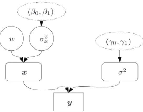
Fig. 2. Graphical representation of proposed Bayesian model.
distributions. The whole model is represented in the direct acyclic graph of Fig. 2 and described hereafter from the bottom to the top of the graph.
Remark 1 (Notations: vector norm).For p ∈ N∗
and x ∈ Cm
the pth norm of x is defined by kxkp
=¡Pm i=1|xi|p
¢1/p
.If p = 0, the norm is defined as the number of non-zero vector elements, i.e., kxk0= # {i ∈
{1, . . . , m}|xi6= 0}.
1) Likelihood:As stated in Section II, the thermal noise n is assumed to be a white Gaussian noise, denoted as n ∼ CN(0, σ2I
KM) with Iξ the ξ × ξ identity matrix.
In other words, when x and σ2are known, the observation
vector is Gaussian distributed, i.e., y|x, σ2
∼ CN(H x, σ2IKM). The likelihood is then given by2
f( y|x, σ2) ∝ 1 σ2KM exp ½ −k y − H xk 2 2 σ2 ¾ (18) where ∝ means proportional to.
2) Parameters:The next level of our model consists in defining the prior probability density functions (pdfs) of the thermal noise power σ2and the K ¯M-length vector x.
a) Prior of σ2:On the mathematical point of view, a convenient prior for σ2is an inverse-Gamma pdf which
belongs to the family of conjugate priors with respect to (wrt) (18) [29]. This pdf is denoted by
σ2|γ0, γ1∼ IG(γ0γ1) and is given by
f(σ2
|γ0, γ1) ∝
e−γ1/σ2 (σ2)γ0+1
I[0,+∞)(σ2) (19)
where IA() denotes the indicator function of the set
A(i.e.,IA(x)=1 if x ∈ A and IA(x) = 0 otherwise), γ0and
γ1represent, respectively, the scale and shape parameters
of the distribution. Then, with an adequate choice for the values of (γ0, γ1), the mean and variance of σ2|γ0, γ1can
be set in accordance with our degree of prior belief about the thermal noise level [30]. For instance, in case of finite
2Note that throughout the paper, constant parameters (e.g., the matrix H)
are not systematically written in the conditional terms for notational convenience.
mean mσ2and variance vσ2,one has
γ0= m2σ2 vσ2 + 2 (20a) γ1= mσ2 Ã m2σ2 vσ2 + 1 ! . (20b)
Particularly for radar applications, the thermal noise power level is often known with a good accuracy as it consists mainly of the receiver thermal noise [1, 31]. Thus, it is reasonable to use (20). Note that the case of a
noninformative prior, i.e., when (γ0, γ1) = (0, 0), has
been presented in [6] and it also gave good performance for the studied scenario.
b) Prior ofx: Assigning a prior pdf to x is a critical
step in the design of our model. For complex data and given the likelihood function (18), a Bernoulli-complex Gaussian distribution appears to be suitable to enforce sparsity in the vector x and to ensure simplicity of the resulting posterior distribution [27, 32, 33]. To be more specific we have assumed that the elements of x, denoted by xi= [x]ifor i = 0, . . . , K ¯M − 1, are a priori
independent and such that
f(xi|w, σx2) = (1 − w) δ(|xi|) + w 1 π σx2exp ½ −|xi| 2 σx2 ¾ (21) with w ∈ [0, 1] and σ2 x >0. The pdf (21), denoted by
xi|w, σx2∼ Ber CN¡w, 0, σx2¢ , is tantamount to assuming
that, at the ith frequency point of analysis, there is no scatterer in the data with a probability (1 – w), while with a probability w there is a scatterer with power3σ2
x.We
stress here that compared with other sparsity inducing priors such as a Laplacian prior [34], samples generated according to (21) can be exactly equal to 0 and that the probability of having a zero element is controlled by the value (1 – w). Recalling the assumption of independence of the xis, the prior distribution of x is given by
f(x|w, σx2) = (1 − w)n0 µ w π σx2 ¶n1 × exp ½ −kxk 2 2 σ2 x ¾ Y i/xi=0 δ(|xi|) (22)
where δ() is the Dirac delta function and
n1= kxk0 and n0= K ¯M − kxk0. (23)
As both the occupancy level w and the scatterer power σx2are not known, another level is defined in the
hierarchical model as detailed hereafter.
3It is observed later that σ2
x can be indeed seen as the postprocessing
3) Hyperparameters:
a) Prior of w:A uniform distribution is chosen for the weight w, denoted as w ∼ U[0,1],i.e.,
f(w) = I[0,1](w) (24)
reflecting the absence of knowledge about w.
b) Prior of σx2: Concerning the power level σ2 x and
according to (21), an inverse-Gamma prior is suitable for further derivation (the same remark was made for the prior of σ2). It is denoted as σ2 x|β0, β1∼ IG(β0, β1) and is given by f¡σx2¯¯β0, β1¢ ∝ e−β1/σx2 σ2(β0+1) x I(0,+∞)¡σx2¢ (25) where β0, β1are, respectively, the shape and scale
parameters. They correspond to the last level of the hierarchical model and are considered as constants set by the radar operator. To choose conveniently their values and thus incorporate adequately prior information about σ2
x in
the model, the following remarks are appropriate. Firstly, according to (21), one has
E{|xi|2|xi6= 0} = σx2 (26)
where E{} is the mathematical expectation. In absence of basis mismatch (17), one also has
E{|xi|2|xi6= 0} = K ¯M × E{|αt|2} (27)
indicating that σ2
x/(K ¯M) can be seen as the average
scatterer power E{|αt|2} before processing. Furthermore,
since β1is a scale parameter, it is straightforward to show
that σ2
x/(K ¯M)|β0, β1∼ IG(β0, β1/(K ¯M)). Hence, when
the radar operator has reliable information about the target power E{|αt|2}—e.g., via the radar equation [1]—that can
be transposed in terms of finite mean mσ2
x/(K ¯M)(i.e.,β0>1) and variance vσ2
x/(K ¯M)(i.e.,β0>2), the shape and scale parameters of (25) can be chosen as follows
β0= m2σ2 x/(K ¯M) vσ2 x/(K ¯M) + 2 (28a) β1= K ¯M mσ2 x/(K ¯M) Ã m2σ2 x/(K ¯M) vσ2 x/(K ¯M) + 1 ! . (28b)
When less or no reliable information is available about the target power, a flat prior can be chosen instead. For instance, when β0, β1→ 0, the pdf reduces to a
noninformative Jeffrey’s distribution [30]. A moderately informative prior is considered later for the numerical simulations allowing for a wide range of target powers. This completes the description of our hierarchical model. B. Bayesian Estimation
Given the Bayesian model described by the set of equations (14), (18), (19), (21), (24), and (25), we propose to derive two conventional Bayesian estimators for the parameter of interest x, namely the MMSE and the MAP
estimators [29, 35]. They are respectively defined as the mean of the posterior distribution and the argument that maximizes this distribution. For the parameter of interest
x, they are thus defined as follows
ˆxMMSE=
Z
xf (x| y)d x (29a) ˆxMAP= arg max
x f(x| y). (29b)
Both rely on the posterior distribution f(x|y) that, according to our hierarchical model, is given by (see the Appendix) f(x| y) ∝ B(1 + n1,1 + n0)Ŵ(β0+ n1) Q i/xi=0δ(|xi|) ¡β1+ kxk22 ¢β0+n1 £k y − H xk2 2+ γ1¤KM+γ0 (30) where B(.) and Ŵ() are the Beta and Gamma functions, respectively.
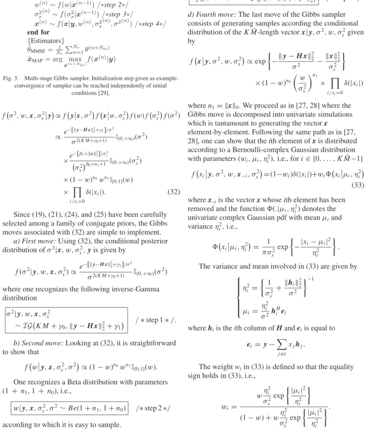
Looking at (30), it seems intractable to derive analytically the MMSE or MAP estimators (29). Moreover, the pdf of x|y (30) does not correspond to a known distribution, making the generation of samples according to x|y not straightforward. We propose therefore to use a common simulation method known as MCMC [29]. More precisely, a multistage Gibbs sampler is implemented [29]. Given our data model, it consists in generating iteratively samples (σ2(n), w(n), σ2(n)
x ,x(n)) that
are distributed according to their respective conditional posterior distributions. After a burn-in period, denoted as
Nbisamples, each subsequence θ(n)4is distributed
according to the posterior distribution θ|y. Collecting enough samples, say a number of Nr, the MMSE and
MAP estimators of x can then be approximated as
xMMSE 1 = N1 r Nr X n=1 x(n+Nbi) (31a)
ˆxMAP= arg1 max {x(n+Nbi )}Nr
n=1
f(x(n)| y). (31b)
Note that while the posterior pdf of x (30) is too complex to obtain a closed-form expression of the MAP estimator (29b), its expression is necessary to derive (31b) with the sampler. The four iterative steps of our MCMC method are detailed in the next section and summarized in Fig. 3.
1) Gibbs Sampler:The Gibbs sampler considered in this work generates iteratively each chain parameter θ according to its posterior distribution. This distribution can be easily obtained from the joint posterior pdf of σ2,x, w, σ2
x| y whose expression follows from the Bayes
theorem
4The notation θ designates successively σ2, w, σ2 xand x.
Fig. 3. Multi-stage Gibbs sampler. Initialization step given as example: convergence of sampler can be reached independently of initial
conditions [29]. f¡σ2, w,x, σ2 x ¯ ¯y¢ ∝ f ¡ y ¯ ¯x, σ2¢f ¡x ¯ ¯w, σx2¢f (w)f ¡σx2¢f (σ2) ∝ e −[k y−H xk2 2+γ1]/σ2 σ2(KM+γ0+1) I(0,+∞)(σ 2) ×e −[β1+kxk22]/σx2 ¡σ2 x ¢β0+n1+1 I(0,+∞)(σ 2 x) × (1 − w)n0wn1I[0,1](w) × Y i/xi=0 δ(|xi|). (32)
Since (19), (21), (24), and (25) have been carefully selected among a family of conjugate priors, the Gibbs moves associated with (32) are simple to implement.
a) First move:Using (32), the conditional posterior distribution of σ2 |x, w, σx2,y is given by f(σ2| y, w, x, σx2) ∝ e−[k y−H xk 2 2+γ1]/σ2 σ2(KM+γ0+1) I(0,+∞)(σ2) where one recognizes the following inverse-Gamma distribution
σ2| y, w, x, σx2
∼ IG¡KM + γ0, k y − H xk22+ γ1¢ / ∗ step 1 ∗ /.
b) Second move:Looking at (32), it is straightforward to show that
f¡w¯
¯y, x, σx2, σ2¢ ∝ (1 − w)n0wn1I[0,1](w).
One recognizes a Beta distribution with parameters (1 + n1, 1 + n0), i.e.,
w| y, x, σx2, σ2∼ Be(1 + n1,1 + n0) /∗ step 2 ∗/
according to which it is easy to sample.
c) Third move:According to (32), the conditional distribution of σ2 x| y, x, σ 2, wis f¡σ2 x ¯ ¯y, x, σ2, w¢ ∝ e−[β1+kxk22]/σx2 ¡σ2 x ¢β0+n1+1 I[0,+∞)¡σ2 x ¢
from which one recognizes an inverse-Gamma distribution, i.e.,
σx2| y, x, σ2, w ∼ IG¡β0+n1, β1+kxk22
¢
/∗ step 3 ∗/.
d) Fourth move:The last move of the Gibbs sampler consists of generating samples according the conditional distribution of the K ¯M-length vector x| y, σ2, w, σx2given by f¡ x¯ ¯y, σ2, w, σx2¢ ∝ exp ½ −k y − H xk 2 2 σ2 − kxk22 σ2 x ¾ × (1 − w)n0µ w σ2 x ¶n1 × Y i/xi=0 δ(|xi|)
where n1= kxk0. We proceed as in [27, 28] where the
Gibbs move is decomposed into univariate simulations which is tantamount to generating the vector x
element-by-element. Following the same path as in [27, 28], one can show that the ith element of x is distributed according to a Bernoulli-complex Gaussian distribution with parameters (wi, µi, η2i), i.e., for i ∈ {0, . . . , K ¯M−1}
f¡xi ¯ ¯y, σ2, w,x−i, σx2¢ =(1−wi)δ(|xi|)+wi8¡xi ¯ ¯µi, ηi2 ¢ (33) where x–iis the vector x whose ith element has been
removed and the function 8(.|µi, η2i) denotes the
univariate complex Gaussian pdf with mean µiand
variance η2 i,i.e., 8¡xi ¯ ¯µi, ηi2¢ = 1 π σ2 x exp ½ −|xi− µi| 2 η2i ¾ . The variance and mean involved in (33) are given by
η2i = ½ 1 σx2 + khik22 σ2 ¾−1 µi = ηi2 σ2 h H i ei
where hiis the ith column of H and eiis equal to ei = y −
X
j 6=i
xjhj.
The weight wiin (33) is defined so that the equality
sign holds in (33), i.e.,
wi= wη 2 i σ2 x exp½ |µi| 2 η2i ¾ (1 − w) + wη 2 i σx2exp ½ |µi|2 ηi2 ¾.
To summarize, the fourth Gibbs move is defined as follows
∀i∈{0, . . . , K ¯M − 1},
xi| y, σ2, w,x−1, σx2∼ BerCN¡wi, µi, ηi2¢.
/∗ step 4 ∗/
Remark 2 (Details of implementation).Note that to update efficiently the coordinate xiat the nth iteration of
the Gibbs sampler, we proceed as in [28, Appendix B]. By doing so, the computationally intensive matrix product Hx is derived only once at the initialization of the sampler (n = 0). Also given the particular nature of H = TF−1
(15a), the product F−1x(0)is firstly performed via an FFT
and an inverse FFT on, respectively, K and ¯Mpoints. Then, the block-diagonal nature of the matrix T is taken into account to avoid unnecessary null-products when computing T × [F−1x(0)].
IV. NUMERICAL SIMULATIONS
The performance of the proposed estimators ˆxMAPand
ˆxMMSEdefined in (31) is firstly assessed with synthetic
radar data generated according to (1). Results are compared with that of an ℓ1penalized least squares
approach which is more conventional when dealing with sparse recovery. More specifically, the ACAMP (adaptive complex approximate message passing) method has been chosen [14, 36, 37]. ACAMP is an iterative thresholding technique that uses a few computations per iteration and offers an adaptive way to optimally set its threshold parameter [14].
A. Simulation Parameters
1) Reference Scenario:The received signal entails
N = 10 scatterers whose velocities and initial positions
satisfy the no-basis mismatch assumption (17). The scatterers actually represent five targets since three of them are extended in range. For each scatterer, the signal-to-noise ratio (SNR) prior to processing is defined as SN Rt = E{|α t|2} σ2 katk22 KM .
Location and SNR of each scatterer is represented in Fig. 4. Note that the considered SNRs are below the thermal noise level and that the gain of integration is 10 log10(KM) ≈ 24 dB. Also, the argument of the
amplitude αtfor t = 1, . . . , N is drawn from a uniform
distribution in [0, 2π). Other parameters of interest describing the radar scenario are depicted in Table I.
2) Processing Parameters:To process the wideband radar signal with our Bayesian method several parameters need to be adjusted. The virtual sampling frequency fr is
chosen 1) high enough to ensure that a target with maximum velocity vmaxcan be estimated without aliasing,
and 2) not too high to limit the computational load that is related directly to the length of the vector x to be
estimated. A good compromise it thus to set frequal to the
Nyquist rate [38] which is tantamount to considering that
Fig. 4. Locations and SNRs of synthetic targets. Range resolution is δR= 15 cm and ambiguous velocity is va= 15 m/s.
TABLE I
Scenario Parameters for Synthetic Data
carrier fc= 10 GHz bandwidth B = 1 GHz PRF fr= 1 kHz # pulses M = 32 LRR segment K = 8 noise power σ2= 1 TABLE II
Processing Parameters for Synthetic Data
σ2prior (γ0, γ1) = (3, 2)
σx2prior (β0, β1/(K ¯M)) ≈ (2.33, 1.33)
max. velocity vmax= 22.5 m/s
virtual PRF f¯r= 3 kHz
virtual # pulses M = 106¯
burn-in Nbi= 50
Gibbs-iterations Nr= 200
an equality sign holds in (8), i.e., ¯fr = 4vmaxfc/c.Then,
the number of virtual pulses ¯Mis chosen 1) high enough to ensure that (10) corresponds to an interpolation formula, and 2) not too high to limit the length of the vector x. Again, a good compromise is to consider that an equality sign holds in (11), i.e., ¯M ≈ ⌈M (1 + B/fc)⌉ ¯fr/fr.This
way, the observation times of both the received and reconstructed signals are identical. Since the values of
¯
frand ¯Mare now fixed, the interpolation-transform
matrix H (15a) is completely defined. Turning then to the values of the hyperparameters (γ0, γ1) and (β0, β1)
involved in the priors of σ2(19) and σ2
x (25), we use the
relations (20) and (28) with (mσ2, vσ2) = σ2(1, 1) and (mσ2
x/(K ¯M), vσx2/(K ¯M)) = σ
2(1, 3). The resulting numerical
values correspond to a rather informative prior for the thermal noise level (which is reasonable for most radar applications) and a moderately informative prior for the average scatterer power (allowing for a wide range of SNRs). Parameters of interest for the processing are gathered in Table II.
B. Performance
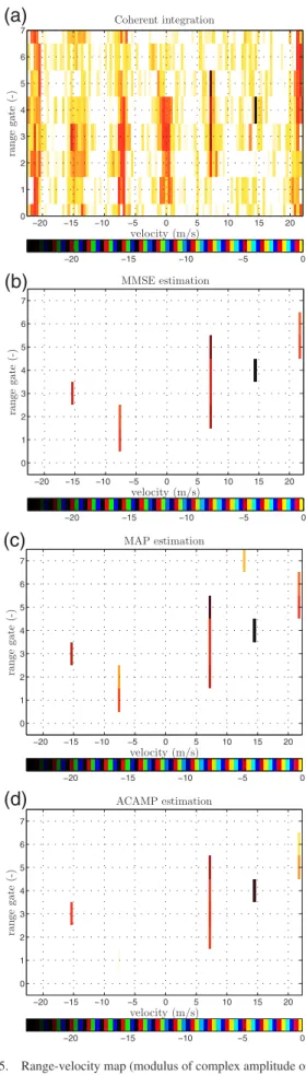
1) Range-Velocity Maps and Histograms:Fig. 5 depicts range-velocity maps of the amplitudes estimated from our Bayesian estimators, the ACAMP algorithm, and a simple coherent integration previously defined in (4). Note that, for a given estimator ˆx, the amplitude vector is defined here by ˆa = ˆx/√K ¯M.Fig. 5(a) shows the limit of using a coherent integration in case of a multitarget scenario since velocity sidelobes are quite high. For instance, though the isolated scatterer around range bin 4 can be well inferred, the target located at range bins 1-2 cannot be clearly distinguished from the sidelobes of the other targets. On the other hand, Figs. 5(b) to 5(d) highlight the interest of using a sparse recovery approach in that case. Indeed, the three CS estimators (MMSE, MAP, ACAMP) of x give a satisfying sparse
representation of the target scene. In particular, no false alarm occurs at the location where sidelobes are expected for a conventional coherent integration. As can be observed (and confirmed by intensive simulations in Section IV-B.2) the MMSE estimator tends to better estimate the target amplitude followed successively by the MAP estimator and the ACAMP method (which mostly underestimates5the target amplitude). Moreover, for all of
these methods, a small amount of non-zero elements that do not correspond to a true scatterer are present. These false alarms are very low for the MMSE (they are even not visible here given the lowerbound of the colorbar), a little bit higher for the ACAMP, and finally more pronounced for the MAP estimator. These preliminary remarks are in favor with the MMSE estimator that better estimates the migrating targets with a few and low false alarms.
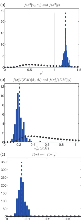
As underlined before, our Bayesian algorithm not only provides a point estimate of x but gives additional information. In particular, histograms and MMSE estimates for σ2, w, σ2
x can be estimated. They are
represented in Fig. 6 and are in accordance with the scenario parameters. Note, that even when the prior is flat, the posterior distribution is clearly tightened around a reliable MMSE estimate. In particular, the estimated level of occupancy is ˆwMMSE= 1.45% while the true level of
occupancy is N/(K ¯M) = 1.18%. In the same vein, the average power of the scatterers present in the scene is
N−1P
tσ2SNRt≈ –5.3 dB while the estimated one is
ˆσ2
x,MMSE/(K ¯M) ≈ −4.5dB. Note also, the accurate
estimation of the thermal noise level ˆσ2
MMSE≈ 0.97.
2) Error of Estimation and Computational Complexity:
The performance of our Bayesian estimators (29) is further investigated by means of Monte-Carlo simulations. Herein, moduli of the target amplitude are kept fixed while their argument as well as the noise are drawn randomly. The performance metric under consideration is the mean absolute error (MAE) defined for an L-length vector θ and
5This is not unconventional for ℓ
1-type solver using a soft thresholding
function. Note in particular that no debiasing technique has been applied to the ACAMP method [39].
Fig. 5. Range-velocity map (modulus of complex amplitude only, in decibels). (a) Coherent integration. (b) MMSE estimation. (c) MAP
Fig. 6. Prior and empirical posterior pdfs. Circle markers represent prior pdfs. Dashed lines represent MMSE estimates. (a) Prior and posterior pdfs of σ2. Plain line represents true value for σ2. (b) Prior and
posterior pdfs of σ2
x. (c) Prior and posterior pdfs of w.
Fig. 7. Performance estimation of studied CS estimators. (a) MAE of ˆx (in decibels). (b) Simulation time per Monte-Carlo run. (c) MAE of target-subvector of ˆx (in decibels). (d) MAE of zero-subvector of ˆx
its estimator ˆθ by
MAE = 1
LE{kθ − ˆθk1}.
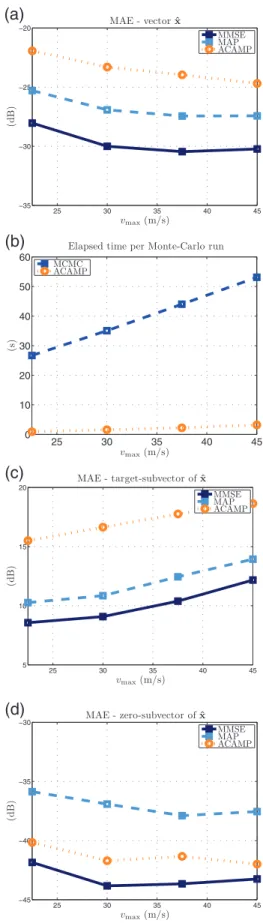
Since the no-basis mismatch hypothesis is assumed (17), the vector x can be split into a zero-subvector and a target-subvector. The MAEs of ˆx and its two subvectors are depicted in Fig. 7 wrt the unfolding parameter vmax. A
general trend can be observed from these three CS estimators: the zero-subvector is slightly better estimated when increasing unfolding, while the contrary is observed for the target amplitude estimation. Then, considering a fixed vmaxand the whole vector ˆx, the lowest MAE is
given by the MMSE estimator, followed successively by the MAP and the ACAMP methods. Considering now the subvectors, it is worth noticing that 1) the MMSE estimator has always the lowest MAE, 2) the MAP estimator better restitutes the target-subvector than the ACAMP method, and 3) an opposite behavior is observed for the zero-subvector: the ℓ1-norm error of the ACAMP
method is lower than that of the MAP estimator and is near to that of the MMSE estimator. Finally, Fig. 7(b) compares the simulation time of both Bayesian and deterministic approaches (for an unoptimized Matlab code). As expected, the greater the unfolding parameter
vmax, the longer the simulation time of each method.
Besides, the good performance of the MMSE technique has to be counterbalanced by its increased computational complexity compared with the ACAMP method.
3) Robustness Towards Grid Mismatch:Before closing this section, a robustness analysis is finally conducted. Grid mismatch is introduced for the Doppler frequency of each simulated scatterer. More specifically, a constant shift δm¯ is applied for t = 1, . . . , N as follows
2vtfc c = ¯ mt+ δm¯ ¯ M ¯ fr
so that the no-basis mismatch assumption (17) is no longer verified. We follow then the path of [40] and estimate the MAE between the estimate ˆx and the vector x which is now incompressible in the dictionary F−1defined in (16).
As can be noticed from Fig. 8, the greater the frequency mismatch, the greater the MAE of the three CS estimators. The MMSE estimator is the most sensitive and its worst MAE is equivalent to that of the ACAMP method. However, this result has to be taken cautiously. Indeed, due to the incompressibility of x, CS estimators split the target power over the vector indices surrounding the true target location. A metric based on a norm error between x and ˆx might not reflect then properly the inherent
detection capability of a given method. This short analysis emphasizes essentially the need for CS approaches (either Bayesian or deterministic) to robustify the estimation towards mismatch grid and/or to design a postprocessing technique to recover the target gain in case of mismatch.
Fig. 8. MAE of CS estimators (MMSE, MAP, ACAMP) wrt Doppler frequency mismatch.
TABLE III
Scenario Parameters for PARSAX Data
carrier fc= 3.315 GHz bandwidth B = 100 MHz PRF fr= 1 kHz # pulses M = 64 LRR segment K = 16 noise power σ2≈ 1
V. SEMIEXPERIMENTAL RADAR DATA
A. Experimental Setup and Processing Parameters Performance of the Bayesian estimators (31) is now assessed on experimental data collected at the Delft University of Technology (TU-Delft). Indeed, the International Research Centre for Telecommunications and Radar (IRCTR) at TU-Delft has been developing over the last years the polarimetric agile radar in S- and X-band (PARSAX) [18]. This system situated on the rooftop of a 100m-high building is continuously upgraded. Recently, data acquired via an S-band linearly frequency modulated continuous waveform (LFMCW) with a bandwidth of
B = 100 MHz has been showing a good dynamic range.
Though the associated range resolution (δR≈ 1.5 m) is not
as high as thought previously in this paper, fast ground moving targets still may migrate of a few range cells during the CPI.
Since no cooperative targets are available in the data, a semiexperimental scenario is under consideration here, i.e., synthetic targets are injected under condition (17) in a presumed free-target region of the PARSAX data. As our Bayesian model assumes that the noise n is white, an ad-hoc prefiltering operation is performed to filter the clutter after target incorporation. It consists of a simple projection on the noise subspace assuming that the clutter has a Gaussian-shape spectrum with adequate bandwidth. The same reasoning as in Section IV-A is then followed to fix the processing parameters of our Bayesian estimators albeit
TABLE IV
Processing Parameters for PARSAX Data
σ2prior (γ0, γ1) = (3,2)
σx2prior (β0, β1/(K ¯M)) ≈ (2.2,1.2)
max. velocity vmax= 55 m/s
virtual PRF f¯r≈ 2.4 kHz
virtual # pulses M = 161¯
burn-in Nbi= 50
Gibbs-iterations Nr= 200
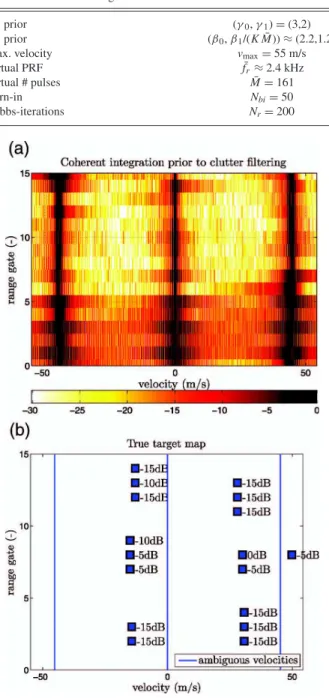
Fig. 9. Semiexperimental data. Range resolution is δR≈ 1.5m and ambiguous velocity is va≈ 45.25 m/s. (a) Coherent integration prior to
target injection and clutter filtering (in decibels). (b) True target map.
1) the expected maximum velocity is fixed to vmax
= 55 m/s to ensure that it is clearly larger than the ambiguous velocity va≈ 42.25 m/s;
2) the variance of σ2
x|β0, β1has been increased to
vσ2
x/(K ¯M)= 5 as it leads to better performance estimation. Note also that prior to target injection, the experimental data have been normalized so that the thermal noise level is approximately equal to σ2
≈ 1. Parameters of interest for the simulation can be seen in Tables III, IV. A representation of the semiexperimental scenario is also depicted in Fig. 9. In particular, location and density of
Fig. 10. Range-velocity map (modulus of complex amplitude only, in decibels). (a) Coherent integration. (b) MMSE estimation. (c) MAP
Fig. 11. Prior and empirical posterior pdfs. Circle markers represent prior pdfs. Dashed lines represent MMSE estimates. (a) Prior and posterior pdfs of σ2. Plain line represents a priori mean
value of σ2. (b) Prior and posterior pdfs of σ2
x. (c) Prior and posterior
pdfs of w.
scatterers in the scenario have been chosen to represent vehicles on a freeway during a heavy traffic time. B. Results
Range-velocity maps obtained from the Bayesian estimators (29) are depicted in Fig. 10 and compared as in the previous section to the amplitude map estimated with the ACAMP method [14]. The target scene recovered by a simple coherent integration (4) is also depicted. The later is clearly highly challenged in dense target environments so that it is hard to tell where the targets are. Note furthermore in Fig. 10(a) the deep notches located not only at the zero-velocity but also at the ambiguous velocities ± va. They indeed have been created by the
clutter prefiltering operation. This ad-hoc filter does not allow—at least for now given the current bandwidth of the PARSAX system—target at the ambiguous velocities to be detected. Concerning the CS estimators, same comments can be made as for the purely synthetic data. The MMSE, MAP, and ACAMP estimates of x give an adequate sparse representation of each scatterer: the MMSE technique gives the best target scene representation; a few false alarms can still be observed for the MAP estimator; the ACAMP method tends again to underestimate target amplitudes.
Histograms and MMSE estimates in Fig. 11 show that the estimation of the thermal noise level, i.e.,
ˆσ2
MMSE≈ 1.23, may have been slightly erroneous while
normalizing the experimental data. This might explain why a better estimation of x is obtained when the prior of the scatterer power σ2
x/(K ¯M) has a larger variance (recall
that its mean has been adjusted to σ2
= 1 in the
simulation). Note that the estimated level of occupancy is ˆ
wMMSE≈ 0.74% which seems reasonable given that the
true level is now N/(K ¯M) = 0.66%. Finally, the average power of the scatterers present in the scene is N−1P
t
σ2SNRt≈ –7.8 dB while the estimated value is
ˆσ2
x,MMSE/(K ¯M) ≈ −6.8dB.
VI. CONCLUSION AND PERSPECTIVES
In case of a low PRF wideband waveform, we have interpreted the target signature as the undersampled version of a virtual but nonaliased bidimensional cisoid. Within a compressive sensing framework, we have proposed accordingly a new Bayesian algorithm able to give an adequate representation of multiple scatterer echoes. By adequate, we mean that each scatterer is represented by a single peak without sidelobe (under the no-basis mismatch assumption). Furthermore, this peak is localized unambiguously in velocity and range at the true velocity and initial round-trip delay of the scatterer. Ambiguity is actually removed thanks to the additional information brought by the range migration. Performance of the Bayesian method (especially, the MMSE
estimation) obtained with synthetic and semiexperimental data is very encouraging.
The price to pay with the proposed method is its computational complexity, which might be reduced using other MCMC methods or variational Bayes algorithms. Upcoming work may also include an extension of our hierarchical Bayesian model to handle grid mismatch (e.g., via the introduction of small perturbations on the dictionary matrix) and colored noise. Modeling colored noise could be an alternative to the ad-hoc filtering technique proposed in this paper to remove clutter from the experimental data. Finally, the proposed Bayesian estimators would deserve to be fully integrated in a whole compressed sensing detection scheme.
APPENDIX. POSTERIOR DISTRIBUTION OF x|y We derive in this Appendix the posterior distribution of x given the observation y. First, note that according to the Bayes theorem, the posterior pdf can be rewritten as
f(x| y) ∝ f ( y|x)f (x). (34) Then integrating the likelihood (18) over σ2given the
prior (19) yields f( y|x) = Z f( y|x, σ2)f (σ2) dσ2 ∝ Z e−[k y−H xk22+γ1]/σ2 (σ2)KM+γ0+1 dσ 2 ∝£k y − H xk22+ γ1¤−(KM+γ 0) (35) Furthermore, the marginal distribution of x is given by f(x) = Z Z f¡ x¯¯w, σx2¢f (w)f ¡σx2¢ dw dσx2 ∝ Z (1 − w)n0wn1I [0,1](w) dw × Z e−[kxk2 2+β1]/σx2 (σ2 x)n1+β0+1 I[0,+∞]¡σx2¢ dσx2× Y i/xi=0 δ(|xi|) ∝ B(1 + n1,1 + n0)Ŵ(β0+ n1) ¡β1+ kxk22 ¢β0+n1 Y i/xi=0 δ(|xi|) (36)
Finally plugging (35) and (36) in (34) yields the expression (30) of the posterior distribution of x|y. ACKNOWLEDGMENT
The authors would like to thank H. Rhzioual Berrada and A. Tamalet for the simulations conducted during their internship. They are also very grateful to O. Besson for many fruitful discussions about this work and to O. Krasnov at TU Delft for kindly providing the PARSAX experimental data.
REFERENCES [1] Skolnik, M. I.
Radar Handbook. New York: McGraw-Hill, 1970. [2] Richards, M. A.
Fundamentals of Radar Signal Processing. New York: McGraw-Hill, 2005.
[3] Trunk, G. V., and Brockett, S.
Range and velocity ambiguity resolution.
In Proceedings of IEEE Radar Conference, Lynnfield, MA, Apr. 1993, pp. 146–149.
[4] Le Chevalier, F. Radar non ambigu `a large bande. French Patent 9 608 509, 1996.
[5] Le Chevalier, F.
Principles of Radar and Sonar Signal Processing. Norwood, MA: Artech House, 2002.
[6] Bidon, S., Tourneret, J.-Y., and Savy, L.
Sparse representation of migrating targets in low PRF wideband radar.
In Proceedings of IEEE Radar Conference, Atlanta, GA, May 7–11, 2012.
[7] Donoho, D. L. Compressed sensing.
IEEE Transactions on Information Theory, 52, 4 (Apr. 2006), 1289–1306.
[8] Cand`es, E. J., and Wakin, M. B.
An introduction to compressive sampling.
IEEE Signal Processing Magazine, 25, 2 (Mar. 2008), 21–30. [9] Berger, C. R., Zhou, S., and Willett, P.
Signal extraction using compressed sensing for passive radar with OFDM signals.
In Proceedings of International Conference on Information
Fusion, Cologne, Germany, June 30-July 3, 2008, pp. 1–6. [10] Ender, J. H. G.
On compressive sensing applied to radar.
Signal Processing, 90, 5 (May 2010), 1402–1414. [11] Herman, M. A., and Strohmer, T.
High-resolution radar via compressed sensing.
IEEE Transactions on Signal Processing, 57, 6 (June 2009), 2275–2284.
[12] Potter, L. C., Ertin, E., Parker, J. T., and C¸ etin, M. Sparsity and compressed sensing in radar imaging.
Proceedings of the IEEE, 98, 6 (June 2010), 1006–1020. [13] Proceedings of the 1st International Workshop on Compressed
Sensing Applied to Radar, Bonn, Germany, May 14–16, 2012.
[14] Anitori, L., Maleki, A., Often, M., Baraniuk, R. G., and Hoogeboom, P.
Design and analysis of compressed sensing radar detectors.
IEEE Transactions on Signal Processing, 61, 4 (Feb. 2013), 813–827.
[15] Parker, J. T., and Potter, L. C.
A Bayesian perspective on sparse regularization for STAP post-processing.
In Proceedings of IEEE Radar Conference, May 10–14, 2010, pp. 1471–1475.
[16] Fuchs, J.-J., and Le Chevalier, F.
D´etection d’une cible mobile en pr´esence de fouillis `a l’aide d’un radar large bande.
In Proceedings of GRETSI, Vannes, France, Sept. 1999, pp. 531–534.
[17] Ji, S., Xue, Y., and Carin, L. Bayesian compressive sensing.
IEEE Transactions on Signal Processing, 56, 6 (June 2008), 2346–2356.
[18] Krasnov, O. A., Babur, G. P., Wang, Z., Ligthart, L. P., and van der Zwan, F.
Basics and first experiments demonstrating isolation improvements in the agile polarimetric FM-CW radar – PARSAX.
International Journal of Microwave and Wireless Technologies(special issue), 2, 3–4 (Aug. 2010), 419–428. [19] Jiang, N., Wu, R., and Li, J.
Super resolution feature extraction of moving targets.
IEEE Transactions on Aerospace and Electronic Systems, 37, 3 (July 2001), 781–793.
[20] Jiang, N., and Li, J.,
Multiple moving target feature extraction for airborne HRR radar.
IEEE Transactions on Aerospace and Electronic Systems, 37, 4 (Oct. 2001), 1254–1266.
[21] Bidon, S., Savy, L., and Deudon, F.
Fast coherent integration for migrating targets with velocity ambiguity.
In Proceedings of IEEE Radar Conference, Kansas City, MO, May 23–27, 2011.
[22] Iverson, D. E.
Coherent processing of ultra-wideband radar signals.
Proceedings of IEE - Radar, Sonar and Navigation, 141, 3 (June 1994), 171–179.
[23] Perry, R. P., DiPietro, R. C., and Fante, R. L. SAR imaging of moving targets.
IEEE Transactions on Aerospace and Electronic Systems, 35, 1 (Jan. 1999), 188–200.
[24] Lush, D. C., and Hudson, D. A.
Ambiguity function analysis of wideband radars.
In Proceedings of 1991 IEEE National Radar Conference, Los Angeles, CA, Mar. 12–13, 1991, pp. 16–20.
[25] Shannon, C. E.
Communications in the presence of noise.
Proceedings of the IRE, 37 (Jan. 1949), 10–21 [26] Abolghasemi, V., Ferdowsi, S., and Sanei, S.
A gradient-based alternating minimization approach for optimization of the measurement matrix in compressive sensing.
Signal Processing, 92, 4 (Apr. 2012), 999–1009. [27] Cheng, Q., Chen, R., and Li, T.-H.
Simultaneous wavelet estimation and deconvolution of reflection seismic signals.
IEEE Transactions on Geoscience and Remote Sensing, 34, 2 (Mar. 1996), 377–384.
[28] Dobigeon, N., Hero, A. O., and Tourneret, J.-Y.
Hierarchical Bayesian sparse image reconstruction with application to MRFM.
IEEE Transactions on Image Processing, 18, 9 (Sept. 2009), 2059–2070.
[29] Robert, C. P., and Casella, G.
Monte Carlo Statistical Methods (Springer Texts in Statistics). New York: Springer, 2004.
[30] Godsill, S. J., and Rayner, P. J. W.
Statistical reconstruction and analysis of autoregressive signals in impulsive noise using the Gibbs sampler.
IEEE Transactions on Speech and Audio Processing, 6, 4 (July 1998), 352–372.
[31] Steiner,M. J., and Gerlach, K.
Fast converging adaptive canceller for a structured covariance matrix.
IEEE Transactions on Aerospace and Electronic Systems, 36, 4 (Oct. 2000), 1115–1126.
[32] Dai, G.-Z., and Mendel, J. M.
Maximum a posteriori estimation of multichannel Bernoulli-Gaussian sequences.
IEEE Transactions on Information Theory, 35, 1 (Jan. 1989), 181–183.
[33] Kormylo, J. J., and Mendel, J. M.
Maximum likelihood detection and estimation of Bernoulli-Gaussian processes.
IEEE Transactions on Information Theory, 28, 3 (May 1982), 482–488.
[34] Tibshirani, R.
Regression shrinkage and selection via the Lasso.
Journal of the Royal Statistical Society, Series B (Methodological), 58, 1 (1996), 267–288. [35] Kay, S. M.
Fundamentals of Statistical Signal Processing: Estimation Theory. Englewood Cliffs, NJ: Prentice-Hall, 1993. [36] Donoho, D. L., Maleki, A., and Montanari, A.
Message-passing algorithms for compressed sensing.
Proceedings of National Academy of Sciences of the United States of America, 106, 45 (2009), 18914–18919. [37] Maleki, A., Anitori, L., Yang, Z., and Baraniuk, R.
Asymptotic analysis of complex LASSO via complex approximate message passing (CAMP).
IEEE Transactions on Information Theory, 59, 7 (2013), 4290–4308.
[38] Oppenheim, A. V., and Schafer, R. W.
Discrete-Time Signal Processing(Prentice-Hall Signal Processing Series). Upper Saddle River, NJ: Prentice-Hall, 1989.
[39] Moghaddam, B., Weiss, Y., and Avidan, S.
Spectral bounds for sparse PCA: Exact and greedy algorithms. In
Advances in Neural Information Processing Systems. Cambridge, MA: MIT Press, 2006, pp. 915–922. [40] Chi, Y., Scharf, L. L., Pezeshki, A., and Calderbank, A. R.
Sensitivity to basis mismatch in compressed sensing.
IEEE Transactions on Signal Processing, 59, 5 (May 2011), 2182–2195.
St´ephanie Bidon (M’08) received the engineer and master degrees from ENSICA,
Toulouse, in 2004 and 2005, respectively, and the Ph.D. degree from INP, Toulouse, in 2008.
She is now with the Department of Electronics, Optronics and Signal of ISAE (Institut Sup´erieur de l’A´eronautique et de l’Espace, Toulouse) as an assistant professor.
Her research interests include digital signal processing particularly with application to airborne radar.
Jean-Yves Tourneret (SM’08) received the ing´enieur degree in electrical engineering
from the Ecole Nationale Sup´erieure d’Electronique, d’Electrotechnique,
d’Informatique, d’Hydraulique et des T´el´ecommunications (ENSEEIHT) de Toulouse in 1989 and the PhD degree from the National Polytechnic Institute from Toulouse in 1992.
He is currently a professor in the university of Toulouse (ENSEEIHT) and a member of the IRIT laboratory (UMR 5505 of the CNRS). His research activities are centered around statistical signal and image processing with a particular interest in Bayesian and Markov chain Monte Carlo methods. He has been involved in the organization of several conferences including the European Conference on Signal Processing (EUSIPCO) in 2002 (as the program chair), the International Conference ICASSP’06 (in charge of plenaries), and the Statistical Signal Processing Workshops SSP’12 (for international liaisons). He has been a member of different technical committees including the Signal Processing Theory and Methods (SPTM) committee of the IEEE Signal Processing Society (2001-2007, 2010-present). He has been serving as an associate editor for the IEEE Transactions on Signal Processing (2008-2011).
Laurent Savy is currently senior advisor of radar systems at ONERA Radar &
Electromagnetism Department since 2007. He started at Thomson Radar Application Centre in 1989, in advanced studies in signal processing. From 2000-2006, he was also with Thales Airborne Systems, responsible for the advanced studies team in the radar technical directorate. His field of interest concerns new concepts in radar and signal processing.
Dr. Savy is author of several papers and patents, in particular regarding STAP (space time adaptive processing) and ATR (automatic target recognition).
Franc¸ois Le Chevalier is in charge of the Chair “Radar Systems Engineering” at Delft
University of Technology, The Netherlands, and Scientific Director of Thales Air Operations Division in Rungis (94), France.
A French pioneer in adaptive digital beamforming and STAP radar systems demonstrations, his current research activities include space-time coding for active antenna systems, and wideband unambiguous radar systems. He has been active in- or chairing- the Technical Program Committees of most IEEE International Radar Conferences since Brest, 1999, has recently chaired the Technical Program Committee of EURAD 2012, Amsterdam, and will be the Honorary Chair of SEE/IEEE
International Radar Conference in France, 2014.
An author of many papers, tutorials, and patents in radar and electronic warfare, Prof. Le Chevalier is the author of Radar and Sonar Signal Processing Principles (Artech House, 2002), editor of Non-Standard Antennas (Wiley, 2010), and co-author of Principles of Modern Radar: Advanced Techniques (Scitech, IET Publishing, 2012).