HAL Id: hal-02530206
https://hal.inria.fr/hal-02530206v2
Submitted on 24 Aug 2020
HAL is a multi-disciplinary open access
archive for the deposit and dissemination of
sci-entific research documents, whether they are
pub-lished or not. The documents may come from
teaching and research institutions in France or
abroad, or from public or private research centers.
L’archive ouverte pluridisciplinaire HAL, est
destinée au dépôt et à la diffusion de documents
scientifiques de niveau recherche, publiés ou non,
émanant des établissements d’enseignement et de
recherche français ou étrangers, des laboratoires
publics ou privés.
RDF graph summarization for first-sight structure
discovery
François Goasdoué, Pawel Guzewicz, Ioana Manolescu
To cite this version:
François Goasdoué, Pawel Guzewicz, Ioana Manolescu. RDF graph summarization for first-sight
structure discovery. The VLDB Journal, Springer, 2020, 29 (5), pp.1191-1218.
�10.1007/s00778-020-00611-y�. �hal-02530206v2�
FIRST-SIGHT STRUCTURE DISCOVERY
FRANC¸ OIS GOASDOU ´E, PAWE L GUZEWICZ, AND IOANA MANOLESCU
Abstract. To help users get familiar with large RDF graphs, RDF summarization techniques can be used. In this work, we study quotient summaries of RDF graphs, that is: graph summaries derived from a notion of equivalence among RDF graph nodes. We make the following contri-butions: (i) four novel summaries which are often small and easy-to-comprehend, in the style of E-R diagrams; (ii) effi-cient (amortized linear-time) algorithms for computing these summaries either from scratch, or incrementally, reflecting ad-ditions to the graph; (iii) the first for-mal study of the interplay between RDF graph saturation in the presence of an RDFS ontology, and summarization; we provide a sufficient condition for a highly efficient shortcut method to build the quo-tient summary of a graph without sat-urating it; (iv) formal results establish-ing the shortcut conditions for some of our summaries and others from the liter-ature; (v) experimental validations of our claim within a tool available online.
1. Introduction
The Resource Description Framework (RDF) is the data model recommended by the W3C for data publishing and sharing data. An RDF graph typ-ically consists of data triples, stating that a sub-ject has a property with a certain value, called ob-ject. An RDF graph may also contain type triples, stating that some resource has the W3C standard rdf:type property (type for short) whose value is a certain type (or, equivalently, class). Finally, an RDF graph may also contain an ontology, describ-ing relationships that hold between the properties and classes present in the graph. For instance, u1
hasName “Julie”, u1 worksFor “ACME” describe
a resource whose identifier (URI) is u1, while u1
type Person assigns it a type; we use quote-enclosed strings to denote constants (also called literals). An ontology associated to this sample dataset may state e.g., that worksFor rdfs:domain Employee: this means “anyone who works for something is of
Date: Accepted on April 1, 2020 for publication in VLDB Journal.
ployee also holds in the above graph, although it is not explicitly written there. Such a triple is called implicit (or inferred, or entailed).
RDF graphs enable describing large and hetero-geneous data sets, which may be hard to understand by human users, and to analyze by machines. To help address this difficulty, many RDF summariza-tion techniques have been proposed in the litera-ture [7], some of which draw upon graph summa-rization techniques [29] proposed independently of RDF. As stated in [7], RDF summarization tech-niques fall into four classes: (i) structural meth-ods are built considering first and foremost the graph structure, respectively the paths and sub-graphs present in the graph; (ii) pattern mining methods apply mining techniques to discover pat-terns in the data and use the patpat-terns as a summary (synthesis) of the graph; (iii) statistical methods aim at extracting from the graph a set of quan-titative measures or statistics; finally (iv) hybrid methods combine elements from more than one of the previous classes. For what concerns summary applications, these range from (RDF) graph index-ing, query cardinality estimation, to helping users formulate graph queries, graph visualization and ex-ploration.
A large and useful class of structural graph sum-maries are based on defining an equivalence rela-tion among graph nodes, and creating one summary node for each equivalence class (set of nodes equiv-alent to each other in the original graph). Then, for every edge labeled p which goes from s to o in the graph, the summary has an edge labeled p from the summary node corresponding to the equiv-alence class of s, to the node corresponding to the equivalence class of p. Such summaries, also called quotient summaries, have many good properties, mainly due to the existence of a graph homomor-phism from the original graph into its summary. Quotient summaries proposed for general graphs in-clude [21, 30, 22, 23, 10, 11].
Summarizing RDF graphs raises two new ques-tions w.r.t. to prior (non-RDF) graph summariza-tion setting: (i) how to take into account the types that may be attached to the nodes (knowing that a node may have no type, or one type, or several)? On one hand, types bring an opportunity to de-fine node equivalence, since, intuitively, two nodes having the same type(s) are likely similar in sole way. On the other hand, they cannot be solely re-lied upon, because many RDF graphs lack types for many (or all) of their nodes; prior RDF sum-mary quotients [37, 35, 5] answer this question in different ways; (ii) how should a summary reflect the implicit triples that may hold in the graph due
to the presence of an ontology? Our prior poster paper [8] is the only work to have addressed this so far.
In this work, we make several theoretical and practical contributions to the area of quotient RDF graph summarization. Specifically:
(1) We formalize an RDF quotient summariza-tion framework, taking into account RDF-specific concepts such as ontologies. (2) We introduce two novel equivalence
rela-tions between RDF nodes, which rely on the transitive co-occurrence of properties on graph nodes. Based on them we de-fine two novel summaries called Weak and Strong respectively, as well as two versions thereof which give priorities to types (for those nodes that have type information); we call these summaries Typed Weak and Typed Strong, respectively. The interest of these new equivalence relations is that they lead to summaries that are much more com-pact (fewer nodes and edges) than quotient summaries previously studied in the litera-ture [21, 30, 22, 23, 10, 11, 37, 35, 5]. This compactness comes at the price of some loss of accuracy. Nevertheless, they do pre-serve a significant amount of information from the input graph. In particular, for domain-specific graphs, describing applica-tions from a specific area, our summaries are very convenient data discovery tools: a simple summary visualization helps learn a lot about the graph structure. This is why our work’s main target are domain-specific graphs. For encyclopedic graphs, such as DBPedia or YAGO, our quotients are very likely to be more compact than some stud-ied in prior work, but still too large for human comprehension; non-quotient sum-maries, e.g., based on pattern mining [7], are more appropriate for such graphs. (3) We are the first to show that for a large
set of RDF equivalence relations, one can build the quotient summary of an RDF graph including its implicit triples, without materializing them. Based on our frame-work, we provide a novel sufficient condi-tion for an RDF equivalence relacondi-tion, which enables building this through our so-called shortcut method; its advantage is to reduce very significantly the summarization time. We prove that our Weak and Strong sum-maries satisfy this condition, whereas the Typed Weak and Typed Strong ones do not; we provide a set of similar results also on previously studied equivalence relations.
(4) Our fourth contribution is a set of novel al-gorithms for computing our summaries, in-cluding incremental ones which are able to reflect the addition of triples to the graph, without re-traversing the rest of the graph. All our algorithms have amortized linear complexity in the size of the graph.
(5) We have implemented these algorithms and summary visualizations in a system called RDFQuotient, available online in open source1.
Sample summary visualization Below, we show an example where our summarization techniques compress an RDF graph structure by many orders of magnitude, while still supporting an informative visualization.
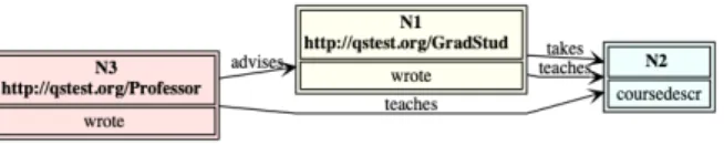
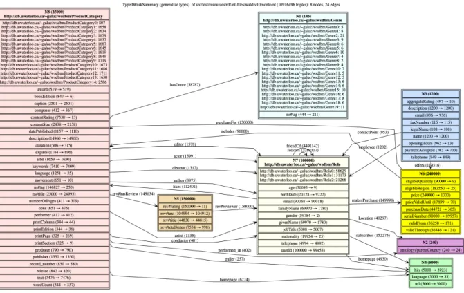
Figure 1 shows the summary of a WatDiv [2] benchmark graph of approximately 11 millions of triples. This visualization reflects the complete structure of the graph, using only 8 nodes and 24 edges, comparable to a simple Entity-Relationship diagram. This summary reads as follows. (i) Non-leaf graph nodes belong to one of the eight disjoint entities, each represented by a summary node (box in Figure 1) labeled N 1 to N 8. The number of graph nodes in each entity appears in parenthesis af-ter the label N i of their representative, e.g., 25000 for N 8. (ii) Each entity represents either graph nodes with types or without types. In the first case, the most general types of the graph nodes, according to which they have been grouped in the entity, are given in bold underneath the entity la-bel; these coincide with the original graph node types when an ontology is not present. For in-stance, all the 25000 graph nodes represented by N 8 are (implicitly) of type ProductCategory due to the ontology at hand; their distribution according to their original typing is also shown, e.g., 807 are of type ProductCategory0. An entity that does not show types represents untyped graph nodes which have been grouped according to the relationships they have with others, using a novel transitive re-lation of co-occurrence of their properties, which we introduce in this paper. For instance, N 4 repre-sents both the web pages of the products of N 8 and these of the persons of N 7, because these web pages can be home pages for both: there are homepage edges from both N 8 to N 4 and from N 7 to N 4. (iii) Graph nodes from an entity may have outgo-ing properties whose values are leaf nodes in the graph; the set of all such properties appears in the corresponding summary node box, one property per line. For each property, e.g., nationality for N 7, the summary node specifies how many graph nodes represented by this entity have it (19924 in this case), and how many distinct leaf nodes are tar-get of these edges (25 in this case). (iv) Graph
Figure 1. ER-style visualization built from one of our summaries.
nodes from an entity may have outgoing properties whose values are non-leaf nodes in the graph. For each graph edge n1
a
−→ n2, where n1, n2are non-leaf
graph nodes and a is the property (edge label), an a-labeled edge in the summary goes from the repre-sentative of n1 to that of n2. Next to a, that
sum-mary edge is also labeled with the number of graph edges to which it corresponds. (v) Properties from a small, fixed vocabulary are considered metadata (as opposed to data) and therefore are not used to split graph nodes in entities, e.g., rdf-schema#comment and rdf-schema#label in Figure 1. More such vi-sualization summaries can be found online1; an
ex-ample leading from an RDF graph to its summary and then such a visualization is worked out in the paper. Most of the material presented here is new. The exceptions are: Theorem 2 appeared without proof in the poster [8]; our algorithms were outlined in the demonstration [15].
Below, Section 2 recalls useful preliminaries, then Section 3 introduces the novel notions of property cliques, based on which we define our summaries. Section 4, respectively, 5 extend this to graphs com-prising type triples, respectively, ontologies. In Sec-tion 6 we discuss summary visualizaSec-tion. SecSec-tion 7 describes our summarization algorithms and Sec-tion 8 presents our experiments. We then survey related work and conclude. Proofs of the technical results of this paper can be found in the Appendix.
Figure 2. Sample RDF graph.
2. Preliminaries
We recall here the starting points of our work: RDF graphs (Section 2.1) and graph quotients (Sec-tion 2.2).
2.1. Data graphs. An RDF graph is a set of triples of the form s p o. A triple states that its sub-ject s has the property p, and the value of that property is the object o. We consider only well-formed triples, as per the RDF specification [38], using uniform resource identifiers (URIs), typed or untyped literals (constants) and blank nodes (un-known URIs or literals). Blank nodes are essen-tial features of RDF allowing to support unknown URI/literal tokens. These are conceptually similar to the labeled nulls or variables used in incomplete relational databases [1], as shown in [16].
As our running example, Figure 2 shows a sam-ple RDF graph G describing a university depart-ment, including professors, graduate students, ar-ticles they wrote, and courses they teach and/or take. Here and in the sequel, nodes shown in gray are classes (or types). Further, nodes whose labels appear enclosed in quotes, e.g., “d1”, are literals, while the others are URIs.
RDFS ontology. One can enhance the resource descriptions comprised in an RDF graph by declar-ing ontological constraints between the classes and the properties they use. For instance, one may add to the graph in Figure 2 the ontology O consisting of the triples
GradStud rdfs:subClassOf Instructor takes rdfs:range Course Professor rdfs:subClassOf Instructor takes rdfs:domain Student
advises rdfs:subPropertyOf knows
to state that graduate students, respectively pro-fessors, are instructors, that anyone who takes a course is a Student, what can be taken is a course, and that advising someone entails knowing him or her.
From ontological constraints and explicit triples, implicit triples may be derived. For instance, from G and O, it follows that p1 is of type Instructor,
which is modeled by the implicit triple p1 type
In-structor; we say this triple holds in G, even though it is not explicitly part of it. Other implicit triples obtained from this ontology based on G are: p2type
Instructor, p2type Student, and p1knows p2. Given
a graph G (which may include a set of ontological constraints, denoted O), the saturation of G, is ob-tained by adding to G: (i) all the implicit triples de-rived from G and O, then (ii) all the implicit triples derived from those of step (i) and O, and so on, un-til a fixpoint, denoted G∞, is reached. These triples are added based on RDF entailment rules from the RDF standard. In this work, we consider the widely-used RDFS entailment rules. They exploit the simple RDFS ontology language, based on the four standard properties illustrated above, which we denote subClass, subProperty, domain and range, to add new ontological constraints or facts. The saturation G∞of any graph G comprising RDFS ontological constraints is finite, unique, and can be computed in polynomial time, e.g., by leveraging a database management system [16]. Crucially, G∞ materializes the semantics of G.
Terminology and notations. We call the triples from G whose property is (rdf:)type type triples, those whose property is among the standard four RDFS ones schema triples, and we call all the other data triples. We say a node is typed in G if the node is the subject of at least one type triple in G. In the graph shown in Figure 2, p1 type Professor is a type triple, hence the node p1 is typed, p1 advises p2 is a data triple, while Professor rdfs:subClassOf Instructor may be a schema triple. Further, we say
a URI from G is a class node if (i) it appears as subject or object of a subClass triple, or an object of range or domain triple; or (ii) it appears as the object of a type triple; or (iii) it appears as a sub-ject of a type triple with obsub-ject rdfs:Class. We call property node, a URI appearing (i) as subject or object in subProperty triple, or as a subject of do-main or range triple; or (ii) as a subject of rdf:type triple with object rdf:Property. Together, the class and property nodes are the schema nodes; all non-schema nodes are data nodes. In Figure 2, Profes-sor and GradStudent are class nodes. If we consider the aforementioned ontology O, takes, advises and knows are property nodes. Finally, the a’s, p’s, c’s and d’s nodes are data nodes.
It is important to stress that not all nodes in an RDF graph are typed, e.g., this is only true for p1
and p2 in Figure 2. Further, some nodes may have
several types, in particular due to saturation (e.g., p2 is of types GradStudent and Instructor) but not
only, e.g., p1 could also be of type ForeignStudent
etc.
2.2. Quotient RDF summaries. We recall here quotient RDF summaries as defined in prior work, outline existing work in this area, and discuss their limitations.
Given an RDF graph G and an equivalence rela-tion2 ≡ over the nodes of G, the quotient of G by
≡, denoted G/≡, is the graph having (i) a node for
each equivalence class of ≡ (thus, for each set of equivalent G nodes); and (ii) for each edge n1
a
−→ n2
in G, an edge m1 a
−→ m2, where m1, m2are the
quo-tient nodes corresponding to the equivalence classes of n1, n2respectively. Quotients have several
desir-able properties from a summarization perspective: Size guarantees:: By definition, G/≡ is
guaranteed to have at most as many nodes and edges as G. Some non-quotient sum-maries, e.g., Dataguides [17], cannot guar-antee this.
Property completeness:: Every property (edge label) from G is present on some sum-mary edges. This gives first-time users of the dataset a chance to decide, based on their interest and envisioned application, if it is worth further investigation. In some applications, e.g., when data journalists ex-plore open data, or physicians look for a rare diagnosis, it is important not to miss a “weak signal”, encoded in RDF as a set of triples using infrequent properties.
Structural homomorphism:: It is easy to see that the function f associating to any
2An equivalence relation ≡ is a binary relation that is reflexive, i.e., x ≡ x, symmetric, i.e., x ≡ y ⇒ y ≡ x, and transitive, i.e., x ≡ y and y ≡ z implies x ≡ z for any x, y, z.
G node, its representative in G/≡ is a
ho-momorphism from G into its summary: any subgraph of G is “projected” by f into a subgraph of its quotient.
Quotient graph summaries include e.g., [30, 22, 10, 36, 25, 11, 13]; RDF quotient summaries are described in [37, 35, 5].
Bisimilarity is behind most equivalence relations used in these works. Two nodes n1, n2 are forward
bisimilar [21] (denoted ≡fw) iff (i) for every G edge
n1 a
−→ m1, G also comprises an edge n2 a
−→ m2, such
that m1 and m2 are also (forward) bisimilar and
(ii) a similar statement holds, replacing n1, m1with
n2, m2 and vice-versa. While forward bisimilarity
focuses on outgoing edges only, two nodes can also be bisimilar w.r.t. their incoming edges, i.e., back-ward bisimilar (denoted ≡bw). Backward similarity
of two nodes n1, n2 is recursively defined similarly
as above when considering G edges m1 a
−→ n1 and
m2 a
−→ n2. Finally, two nodes can be bisimilar based
on both their incoming and outgoing edges, i.e., for-ward and backfor-ward bisimilar (denoted ≡fb), when
they are both forward bisimilar and backward bisim-ilar. We denote the bisimulation based summaries G/fw (forward), G/bw (backward) and G/fb (forward
and backward), respectively. They have been stud-ied, in particular for indexing and query processing, in [37, 5, 35].
Leaf (resp. root) collapse An issue encountered when summarizing only according to the properties outgoing a node, e.g., ≡fw, is that the summary
con-siders equivalent (thus, collapses) all nodes lacking outgoing edges, that is, all the leaves of G. Such leaf nodes may have very little to do with each other. For instance, on the WatDiv graph summarized in Figure 1, all the values of award, numberOfPages, keywords, email, faxNumber would be summarized together, even though they are very different. We call this situation leaf collapse through summariza-tion. symmetrically, a summary whose relation only depends on nodes’ incoming properties, e.g., ≡bw, automatically summarizes together all nodes with no incoming edges, although again they may repre-sent very different things; we call this root collapse. We argue that a good summary should not system-atically collapse leaves (respectively, roots), but do so only when they really are similar to each other.
Bisimulation summaries tend to be large, be-cause bisimilarity is rare in heterogeneous graphs. For instance, in Figure 2, none of p1, p2, . . . p5 is
bisimilar to the other, due to slight differences in their properties; similarly, the courses c1, c2 and
c3are not bisimilar, because c3lacks a description,
c2 is the only one target of a “takes” triple etc.
Our experiments in Section 8 confirm this on many graphs.
Bounded bisimilarity To mitigate this problem, k-bisimilarity was introduced [23]. For some integer
Figure 3. 1fb summary of the RDF graph in Figure 2.
Figure 4. 1fw summary of the RDF graph in Figure 2.
k, nodes are k-forward (and/or backward) bisimilar iff they are bisimilar within their k-bound neighbor-hoods. One drawback of k-bisimilarity is that it re-quires users to guess the k value leading to the best compromise between compactness (favored by a low k, e.g., if k = 0, all the graph nodes are equivalent, and the summary has a single node) and structural information in the summary (high k). RDF quo-tients based on k-bisimilarity are studied in [37, 5]. It turns out that even 1-bisimilarity is rare in heterogeneous graphs. For instance, Figure 3 shows the 1fb summary of the sample graph in Figure 23. Here and throughout this paper, summary nodes are shown in rectangles and are labeled N1, N2 etc.;
we abridge property names to use w for wrote, a for advises, te for teaches, ta for takes and cd for coursedescr. Nodes N3, N4 and N8 represent,
re-spectively, p1, p2, p3; the three courses are
repre-sented by N1 and N6. This summary is almost as
complex as the input graph. Figure 4 shows the 1fw summary of our sample G: it is smaller (only 5 nodes and 10 edges, whereas the 1fb one has 8 nodes and 12 edges). However, as our experiments show, 1fw summaries are still too large to be useful for visual-ization. The 1fw summary, denoted ∼ain [5], is also
very similar to grouping nodes into “characteristic sets” [18, 32]; they all suffer from the leaf collapse issue described above. For instance, they summa-rize together all articles and course descriptions (N2
in Figure 4).
To avoid too many characteristic sets (or, equiv-alently, to reduce the number of summary nodes), [32] proposes a cardinality-based heuristic method which merges them into maximum r sets, for a user-specified threshold r. We do not burden the user with choosing such a threshold; as our experiments show, some graphs are much more complex than
3The summaries shown in the Figures 3, 4 and 5 ignore the type triples of G for readability and because they were not used for summarization in the referenced works.
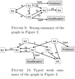
Figure 5. ∼ioa summary [5] of
the RDF graph in Figure 2.
others, thus it is not easy to set r, especially for users not yet acquainted with the data, such as the ones we target.
In [5], any RDF equivalence relation (thus, any RDF quotient) considers all the leaf nodes, whether URIs or literals, as equivalent, and represents them by a single summary node denoted [0]. Thus, all their summaries automatically suffer from the leaf collapse issue. For instance, their 1fb equivalence (denoted ∼ioa) leads to the summary shown in Fig-ure 5. This may significantly reduce the number of summary nodes, since only one of them is a leaf. However, as reported in [5] and verified in our ex-periments, their bisimilarity-based summaries are still too large for visualization.
Type-driven summarization The remaining equivalence relations used in the literature to sum-marize RDF graphs are (also) based on RDF types. In [5], two nodes are ∼t-equivalent if they have
exactly the same types. This collapses all untyped nodes in a single summary node, e.g., all but p1
and p2 in Figure 2, and five out of the eight nodes
in Figure 1 (N2, N3, N4, N5 and N6), even though
they are unrelated.
[5] also introduces ∼ioat, which considers two nodes equivalent iff they are 1fb equivalent and they have exactly the same types. Thus, a ∼ioat summary has at least as many nodes and edges as the ∼ioaone; our experiments confirm it is too large
to be used for first-sight visualization.
To conclude, the equivalence relations used in prior RDF quotient summaries are based on:
(1) Bisimilarity (possibly bounded to a max-imum distance k), which leads to complex summaries with very high numbers of nodes and edges, unsuited for first-sight discovery. (2) Uni-directional bisimilarity (i.e., ≡fw, ≡bw
and their bounded variants), which suffer from leaf or root collapse;
(3) Types alone: this collapses all untyped nodes, even when their data properties have nothing to do with each other;
(4) Bisimilarity and having the same types; this leads to summaries at least as large as those based on bisimilarity alone.
Leaf collapse is also present in all the equivalences of [5].
G RDF graph
G∞ the result of saturating G (Sec-tion 2.1)
type rdf:type (Section 2.1) sc, sp rdfs:subClassOf,
rdfs:subPropertyOf (Section 2.1) domain, range rdfs:domain, rdfs:range
(Sec-tion 2.1)
≡S strong equivalence (Definition 2)
≡W weak equivalence (Definition 3)
G/S strong summary of G (Definition 5)
G/W weak summary of G (Definition 4)
≡TW typed weak equivalence
(Sec-tion 4.2)
≡TS typed strong equivalence
(Sec-tion 4.2)
G/TW typed weak summary of
G(Definition 6)
G/TS typed strong summary of G
(Sec-tion 4.2)
l strong homomorphism (Defini-tion 7)
Table 1. Summary of the notations used in the article.
Another limitation of prior work is not consid-ering how summarization interacts with saturation, and instead simply assuming that G is already sat-urated. When this is not the case, obtaining the summary of G∞ requires first computing this satu-ration, which may be costly in terms of computation time and storage space.
To go beyond these limitations, in the sequel, we introduce our novel equivalence relations, leading to compact and informative quotient summaries of RDF graphs, whether they are fully typed, have no types at all, or are anywhere in between. Further, we provide novel, advanced techniques for summa-rizing a graph’s saturation without saturating it ; this can lead to speed-ups of orders of magnitude. The notations we use in this work are compiled in Table 1.
3. Data graph summarization
We first consider graphs made of data triples only. We define the novel notion of property cliques in Section 3.1; building on them, we devise new graph node equivalence relations and correspond-ing graph summaries in Section 3.2. Summariza-tion will be generalized to handle also type triples in Section 4.
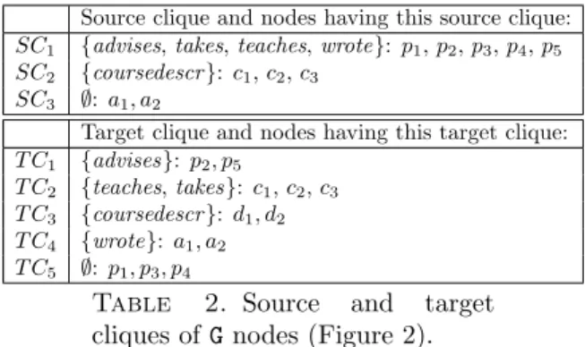
3.1. Data property cliques. Let us consider the ways in which data properties (edge labels) are or-ganized in a graph. The simplest relation is co-occurrence, when a node is the source (or target) of two edges carrying the two labels. However, as illus-trated in Figure 2, two properties, such as wrote and
Source clique and nodes having this source clique: SC1 {advises, takes, teaches, wrote}: p1, p2, p3, p4, p5
SC2 {coursedescr }: c1, c2, c3
SC3 ∅: a1, a2
Target clique and nodes having this target clique: T C1 {advises}: p2, p5
T C2 {teaches, takes}: c1, c2, c3
T C3 {coursedescr }: d1, d2
T C4 {wrote}: a1, a2
T C5 ∅: p1, p3, p4
Table 2. Source and target cliques of G nodes (Figure 2).
advises, may co-occur on one node, while another one may have wrote and teaches. The main intu-ition of our work is to consider all these properties (wrote, advises, teaches) related, as they directly or transitively co-occur on some nodes. Formally:
Definition 1. (Property relations and cliques) Let p1, p2 be two data properties in G:
(1) p1, p2∈ G are source-related iff either: (i) a
data node in G is the subject of both p1 and
p2, or (ii) G holds a data node that is the
subject of p1and of a data property p3, with
p3 and p2 being source-related.
(2) p1, p2∈ G are target-related iff either: (i) a
data node in G is the object of both p1 and
p2, or (ii) G holds a data node that is the
object of p1and of a data property p3, with
p3 and p2 being target-related.
A maximal set of data properties in G which are pairwise source-related (respectively, target-related) is called a source (respectively, target) property clique.
In the graph in Figure 2, properties advises and teaches are source-related due to p4 (condition (i)
in the definition). Similarly, advises and wrote are source-related due to p1; consequently, teaches and
wrote are source-related (condition (ii)). Further, the graduate student p2 teaches a course and takes
another, thus teaches, advises, wrote and takes are all part of the same source clique. Table 2 shows the target and source cliques of all data nodes from Figure 2.
It is easy to see that the set of non-empty source (or target) property cliques is a partition over the data properties of G. Further, if a node n ∈ G is a source of some data properties, they are all in the same source clique; similarly, all the properties of which n is a target are in the same target clique.
3.2. Strong and weak node equivalences. Building on property cliques, we define two node equivalence relations among the data nodes of a graph G:
Definition 2. (Strong equivalence) Two data nodes n1, n2 of G are strongly equivalent, denoted
Figure 6. Weak summary of the RDF graph in Figure 2 (type triples excluded).
n1≡Sn2, iff they have the same source and target
cliques.
Strongly equivalent nodes have the same struc-ture of incoming and outgoing edges. In Figure 2, nodes p1, p3 and p4 are strongly equivalent to each
other. Among these, note that p1 and p3may seem
very dissimilar: p1 has the properties {wrote,
ad-vises} while p3 has only {teaches}. These nodes
are strongly equivalent due to the node p4 which
has a common outgoing property with p1, and one
with p3. Similarly, p2, p5 are strongly equivalent,
and so are c1, c2and c3etc. The transitivity built in
strong equivalence through the use of cliques allows to recognize all these publication nodes as equiv-alent, and avoid separating them (as ≡fb and ≡fw
do, recall Figures 3, 4 in Section 2.2). Thus, clique-based equivalence avoids the pitfall of leading to too many nodes for a readable visualization.
A second, weaker notion of node equivalence re-quests only that equivalent nodes share the same incoming or outgoing structure, i.e., they share the same source clique or the same target clique. For-mally:
Definition 3. (Weak equivalence) Two data nodes n1, n2 are weakly equivalent, denoted n1 ≡W
n2, iff: (i) they have the same non-empty source
or non-empty target clique, or (ii) they both have empty source and empty target cliques, or (iii) they are both weakly equivalent to another node of G.
It is easy to see that ≡Wand ≡S are equivalence relations and that strong equivalence implies weak equivalence, noted ≡S⇒≡W.
In Figure 2, p1, . . . , p5 are weakly equivalent to
each other due to their common source clique SC1;
a1, a2 are weakly equivalent due to their common
target clique etc.
From the definitions above and the equivalence notions recalled in Section 2.2, it follows that ≡1fb
is more restrictive than ≡S (≡1fb⇒≡S⇒≡W).
How-ever, ≡Sand ≡W, which reflect outgoing and
incom-ing properties, are in general incomparable with ≡1fw and ≡1bw, which only outgoing, respectively,
incoming properties. The transitive aspect of prop-erty cliques is a radical departure from previously considered equivalence relations (Section 2). It gives ≡S and ≡W the flexibility to accept as equiv-alent structurally heterogeneous nodes, leading to summaries which are both meaningful and compact.
Figure 7. Strong summary of the RDF graph in Figure 2 (type triples excluded).
Property nodes equivalence We make an im-portant addition to the clique-based equivalences introduced above. A property node (Section 2.1), that is, a node (subject or object) labeled by an URI which also appears as a property of a data node, is only ≡Wand ≡Sto itself. Property nodes are pretty rare, but they do occur in some RDF graphs; an ex-ample would be the subject of a triple such as takes definedBy studentOfficerX, where takes appears as a data property in Figure 2. A triple comprising a property node can be seen as a form of metadata, which helps interpret/understand the graph’s data triples. Thus, we consider that a property node is only equivalent to itself.
3.3. Weak and strong summarization. Weak summarization. The first summary we define is based on weak equivalence:
Definition 4. (Weak summary) The weak sum-mary of a data graph G, denoted G/W, is its quotient
graph w.r.t. the weak equivalence relation ≡W.
The weak summary of the graph in Figure 2 is depicted in Figure 6. N1 represents all the people
(p1to p5), N2represents the courses, N3the articles
and N4 the course descriptions. Note the self-loop
from N1 to itself; it denotes that some nodes
rep-resented by N1 advise some nodes represented by
N1. This summary has only 4 nodes and 5 edges; it
is smaller (at most half as many edges) and much easier to grasp than the 1fb, 1fw and ∼ioa ones,
shown in Section 2. At the same time, it conveys the essential information that some nodes advise, write, also they teach and take something that has course descriptions.
Generally speaking, node Ni in the weak
sum-mary G/W of a graph G represents all the G nodes
whose outgoing (respectively, incoming) properties are a subset of the outgoing (resp., incoming) prop-erties of Ni.
The weak summary has the following important property:
Proposition 1. (Unique data properties) Each G data property appears exactly once in G/W.
We exploit this to efficiently build weak graph summaries (Section 7).
We remark that the weak summary G/W of a
graph G has minimal size (in the number of edges)
among all the quotient summaries of G: every prop-erty labeling a G edge appears exactly once in G/W,
while, by definition, it appears at least once in any quotient summary (Section 2.2). Our experiments show that |G/W| is typically 3 to 6 orders of
magni-tude smaller than |G|.
Strong summarization. Next, we introduce:
Definition 5. (Strong summary) The strong summary of the graph G, denoted G/S, is its quotient
graph w.r.t. the strong equivalence relation ≡S.
The strong summary of the graph of Figure 2 is shown in Figure 7. Similarly to the weak sum-mary (Figure 6), the strong one groups all courses together, and all articles together. However, it sep-arates the person node in two: those represented by N1advise those represented by N2. This is because
the target clique of p1, p3 and p4 is empty, while
the target clique of p2and p5is {advises} (Table 2).
Due to this finer granularity, in G/S, several edges
may have the same label, e.g., there are two teaches and two wrote edges in Figure 7, whereas in G/W,
as stated in Proposition 1, this is not possible. Our experiments (Section 8) show that while G/Sis often
somehow larger than G/W, it still remains many
or-ders of magnitude smaller than the original graph. By definition of ≡S, equivalent nodes have the
same source clique and the same target clique. This leads directly to the next result, exploited by our al-gorithms for building strong summaries (Section 7):
Proposition 2. (Strong summary nodes and G cliques) G/Shas exactly one node for each source
clique and target clique of a same G data node. From the strong to the weak summary. Be-cause strong equivalence implies weak equivalence, it follows that (G/S)/W = G/W. For instance, the
nodes N1and N2 in Figure 7 have the same source
clique, thus the weak summary of the graph in Fig-ure 7 is exactly the one in FigFig-ure 6. Hence, one can get both G/Wand G/Sby building G/Sand then weakly
summarizing it to also get G/W. This is (much) faster
than re-summarizing G, mainly because G/Sis much
smaller than G. Another consequence is that G/W,
in-tuitively, compresses more (is more imprecise) than G/S4; we demonstrate this also through experiments
(Table 6 in Section 8).
Property node representation. Since property nodes represent a form of metadata about the data graph, we decide that in all our quotient summaries they are always represented by themselves, i.e., a node labeled with the same URI.
SameAs and generic properties. Some special properties frequently used in RDF deserve a special
4One example among many: the W summary of a BSBM 1M graph has just one node, whereas the S summary has 5 and is quite informative (https://rdfquotient.inria.fr/ files/2019/11/bsbm1m_s_split_and_fold_leaves.png).
treatment. First, the standard owl:sameAs prop-erty is used to denote that two URIs should be considered as being “the same”; in particular, the incoming/outgoing edges of one should also be con-sidered as belonging to the other. To reflect this special semantics, we extend our notion of clique to treat the properties incoming/outgoing two nodes connected by sameAs (directly or indirectly) as if they occurred on the same node. This ensures that any two nodes connected by sameAs have the same source and target clique, thus they are weakly and strongly equivalent. Second, some generic proper-ties such as rdfs:label are sometimes used to an-notate RDF nodes with very different meaning. Building cliques based on the co-occurrence of such generic properties may consider too many nodes equivalent. To avoid this, we build our cliques ig-noring the triples whose properties are generic, con-struct G/Wor G/Saccordingly, then, for each triple of
the form n1 rdfs:label t (where t is some text), we
add an edge N1rdfs:label N2to the weak or strong
summary, where N1is the representative of n1, and
N2 is a new summary node, representing t.
4. Typed data graph summarization We now discuss the summarization of graphs with data and type triples. Types represent domain knowledge that the data producers found meaning-ful to describe it. However, some or all nodes of a graph may lack types.
Only a few RDF graph summarization works ex-plicitly considered type triples. The equivalence relation ∼t introduced in [5] follows an approach
we call type-only: nodes are equivalent if they have exactly the same types. This approach groups to-gether all untyped nodes, which is problematic in graphs such as the one summarized in Figure 1. The same approach is taken in [27] which further assumes that all non-leaf nodes are typed, a sup-position not borne out in practice (see again Fig-ure 1). A different approach we term data-and-type is taken in [5]: for two nodes to be equivalent, they should both be equivalent according to a relation that only reflects their data properties, and have the same types. For instance, ∼ioat is based both
on having the same input and output properties (∼ioa), and the same types. As explained in
Sec-tion 2, this splits graph nodes into many equivalence classes (summary nodes), which is not desirable for first-sight visualization.
A better approach introduced in [5] to reflect types in a quotient summary built from an equiv-alence relation ≡ is as follows: first, summarize G ignoring type triples, and second, for each triple n type C in G, add to G/≡a triple N type C, where N
represents n in G/≡. We call this quotient
summa-rization approach data-then-type. It does not suffer
Figure 8. Weak summary of the graph in Figure 2.
from the disadvantages of type-only nor data-and-type. Instead, it allows to identify meaningful node groups even in graphs where some or all the nodes lack types.
Below, we start by formalizing the special treat-ment we argue should be given to class and prop-erty nodes in any RDF quotient summary. Based on this, we extend the data-then-type approach to our clique-based equivalence relations (Section 4.1), then present another novel approach which we call type-then-data. It gives priority to types when avail-able, while still avoiding the pitfalls of type-only and data-and-type summarization (Section 4.2). Class node equivalence and representation. To ensure quotient summaries preserve the applica-tion knowledge encoded within the classes, proper-ties and ontology of a graph, we decide that in any equivalence relation ≡, any class node is only equiv-alent to itself, and any class node is represented by itself, and similarly for property nodes. Hence, a typed data graph has the same class nodes, and the same property nodes (Section 3), as its summary.
4.1. Data-then-type summarization. We ex-tend the W, respectively S summaries to type triples, by stating that they follow the data-then-type ap-proach.
Figure 8 illustrates this for G/W; note that N1
is attached both Professor and GradStudent types. Generally, a typed node Ni in a typed weak
sum-mary represents all the G nodes whose incom-ing/outgoing properties are included in those of Ni,
some of which may also have some of the types of Ni; the G nodes represented by an untyped node Nj
are the same as in a weak summary.
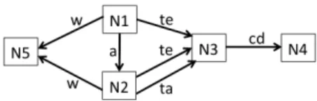
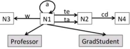
Figure 9 shows the strong summary of our sample graph when type triples are considered. Note that the Professor type is attached to N1, the
represen-tative of p1, p3 and p4(those who advise someone),
while GradStudent is attached to N5, representing
the advisees (p2 and p5).
4.2. Type-then-data summarization. This ap-proach is novel. In contrast with data-then-types, it considers that node types are more important when deciding whether nodes are equivalent, however, it still relies on data properties to summarize untyped nodes. Thus, from an equivalence relation ≡ (based on data properties alone), we derive a novel typed
Figure 9. Strong summary of the graph in Figure 2.
Figure 10. Typed weak sum-mary of the graph in Figure 2.
equivalence relation whereas two nodes are equiva-lent if:
• both are typed, and they have the same set of types;
• or, both are untyped, and they are equiva-lent according to ≡.
For weak summarization, this approach leads to:
Definition 6. (Typed weak summary) Let ≡TW
(typed weak equivalence) be an equivalence rela-tion that holds between two data nodes n1, n2 iff
(i) n1, n2 have no types in G and n1 ≡W n2; or
(ii) n1, n2 have the same non-empty set of types
in G. The typed weak summary G/TW of a graph G
is denoted G/TW.
Figure 10 shows the typed weak summary of our sample RDF graph. Unlike G/W(Figure 6), G/TW
rep-resents p1by N1, separately from p3, because p3 is
of type Person, while p3 is untyped.
In a similar manner, we define typed strong equivalence, denoted ≡TS, as in Definition 6 by
re-placing ≡Wwith ≡S, and denoting by G/TSthe typed
strong summary of a graph G. In our example, G/TS coincides with G/TW.
From the typed strong to typed weak sum-mary. It is easy to see that if n1≡TSn2, then also
n1 ≡TW n2, therefore (G/TS)/TW = G/TW. This also
al-lows building G/TS and G/TW for almost the cost of
building G/TS alone, as this summary is small and
thus summarized quickly.
Summary equality. We now consider when two of our summaries may coincide for a given graph G, i.e., they are the same up to their data node labels N1, N2 etc. To formalize this, we define:
Definition 7. (Strong isomorphism l) A strong isomorphism between two RDF graphs G1, G2,
noted G1l G2, is an isomorphism which is the
iden-tity for the class and property nodes.
We remark that for visualization purposes, strongly isomorphic summaries can be seen as iden-tical, as they describe exactly the same structure.
5. Summarization of graphs with RDFS ontologies
We now turn to the general case of an RDF graph with an RDFS ontology.
First, observe that any summary of an RDF graph has the same RDFS ontology as this graph. This is because: (i) every property node is only rep-resented by itself (Section 3.2), (ii) every class node is represented by itself (Section 3.3), and (iii) by definition of an RDF quotient, any ontology triple, which only connects two class or property nodes, is “copied” in the summary. We view ontology preser-vation as a desirable feature, since the ontology has crucial information about the meaning of the data5. Second, we identify two ways in which an ontol-ogy can impact summarization:
Through type generalization:: Type-then-data summarization (Section 4.2) groups nodes by their sets of types. If the ontology features triples of the form c1 sc c2, it can be argued that c2 can be
used instead of c1 to summarize a resource
having the type c1. We study this in
Section 5.1.
Through implicit triples:: As we ex-plained in Section 2, the semantics of an RDF graph G includes its explicit triples, but also its implicit triples which are not in G, but hold in G∞ due to ontological constraints (such as the triples p2 type
Instructor, p2 type Student, and p1 knows
p2 in Section 2.1). An interesting question,
then, is to determine the interplay between saturation and summarization: how is the summary of G∞ related to that of G, first, in general (for any quotient summary), and then, for the four summaries we introduced? The rest of the section is devoted to this topic.
5.1. Type-then-data summarization using most general types. The most commonly used feature of RDFS ontologies is the subClass relation-ship, stating that any resource of a type c1 is also
of the type c2; “subtype” and “supertype” are
com-monly used to denote c1 and c2 in such settings.
The subgraph consisting of the subClass triples of a graph is typically acyclic (if a loop existed, all the types involved in the loop would be equivalent for
5While we consider the ontology very important, our goal is to bring the much more numerous data and type (non-ontology) triples to a visually comprehensible size through summarization. When present, the ontology may help visu-alize the data; the ontology itself may be summarized etc.
all practical purposes and could be replaced with any among them); we assume below that this is the case, thus the types present in G can be organized in a directed acyclic graph (DAG). While class nodes are very often much fewer than data nodes, they can still be too numerous for a small visualization to include or reflect all of them. For instance, there are more than 500 product types labeled Product-Type1, ProductType2 etc. in a BSBM benchmark graph of 100M triples, a WatDiv benchmark graph of 10M triple comprises 14 product category types, or the real-life DBLP dataset includes a dozen types of scientific publications. Applying type-then-data summarization to such a graph would lead to a high number of nodes, one for each type; this appears shortsighted, given that in these examples, a natu-ral common supertype can be found, e.g., Product-Type, ProductCategory, and Publication, respec-tively.
To obtain compact type-then-data summaries even in the presence of such ontologies, we adopt the following practical solution:
• For each typed data node x ∈ G, let τ (x) be the set of all types associated to x in G, and τ (x) the set comprising the most general supertypes of the types in τ (x)6, which can
be easily computed based on the subClass triples.
• Then, type-then-data summarization based on most general types uses τ (x) instead of τ (x). This is how we obtained the graph in Figure 1: there, N1 represents all the nodes whose most general type set comprises exactly http://db.uwaterloo. ca/~galuc/wsdbm/Genre, and similarly for N8 and the type http://db.uwaterloo. ca/~galuc/wsdbm/ProductCategory. This technique can be applied to both typed weak and typed strong summarization.
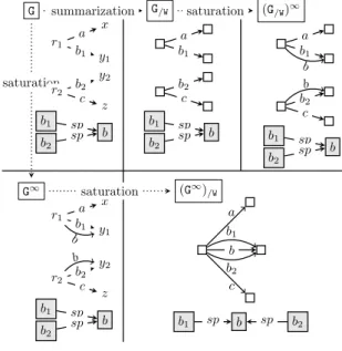
5.2. Interactions between summarization and saturation. First, does saturation commute with summarization? In other words, is (G∞)/≡strongly
isomorphic (Definition 7) to (G/≡)∞? Figure 11
shows that this is not always the case; sp denotes the standard property RDFS rdfs:subPropertyOf (Section 2.1). For a given graph G, the figure shows its weak summary G/Wand its saturation (G/W)∞, as
well as G∞ and its summary (G∞)/W. Here, satura-tion leads to b edges outgoing both r1and r2which
makes them equivalent in G∞. In contrast, sum-marization before saturation represents them sepa-rately; saturating the summary cannot unify them
6We exclude a few “standard” root types, such as rdfs:Resource in RDF Schema or OWL:Thing, from the su-pertype hierarchy, as these would not bring useful informa-tion to summary users.
y2 y1 r1 r2 z x b2 c a b1 b1 b2 b sp sp G a b1 G/W b2 c b1 b2 b sp sp a b1 b (G/W)∞ b2 c b1 b2 b sp sp b r1 x y1 a b1 b G∞ r2 y2 z b2 c b1 b2 b sp sp b b (G∞) /W b1 a b2 c b1 sp b sp b2 saturation summarization saturation saturation r2
Figure 11. Saturation and sum-marization example. (G∞)/ ≡ G∞ f1 ((G/≡)∞)/≡ l by Theorem 2 (G/≡)∞ f2 f homomorph. by Theorem 1 G f repr. fn. of summarizing G G/≡ ∞ ∞ Theorem 2 Theorem 1
Figure 12. Illustration for Theo-rem 1 and TheoTheo-rem 2.
as in (G∞)/W(recall from Section 2.1 that saturation can only add edges in a graph).
While (G∞)/≡ and (G/≡)∞ are not strongly
iso-morphic in general, we establish that they always relate as follows (see the diagram in Figure 12):
Theorem 1. (Summarization homomorphism) Let G be an RDF graph, G/≡ its summary and f the
corresponding representation function from G nodes to G/≡ nodes. Then f defines a homomorphism
from G∞ to (G/≡)∞.
Since (G/≡)∞is homomorphic to G∞, would their
summaries coincide, i.e., be strongly isomorphic? It turns out that this may hold or not depending on the RDF equivalence relation under considera-tion. When it holds, we call shortcut the follow-ing three-step transformation aimfollow-ing at obtainfollow-ing a summary strongly isomorphic to (G∞)/≡, instead
of (G∞)/≡ itself: first summarize G; then saturate
its summary; finally, summarize it again in order to build ((G/≡)∞)/≡:
Definition 8. (Shortcut) We say the shortcut holds for a given RDF node equivalence relation ≡
iff for any G, (G∞)/≡ and ((G/≡)∞)/≡ are strongly
isomorphic.
Note that from a practical viewpoint, hence for visualization, (G∞)/≡ and ((G/≡)∞)/≡ are
equiva-lent as they differ just in their data node IDs (e.g., N1, N2 etc. in Figure 1), which carry no particular meaning.
Next, we establish one of our main contributions: a sufficient condition under which for any quotient summary based on an equivalence relation ≡ as dis-cussed above (where class and property nodes are preserved by summarization), the shortcut holds. In particular, as we will demonstrate (Section 8), the existence of the shortcut can lead to computing (G∞)/≡ substantially faster by actually computing
((G/≡)∞)/≡.
Theorem 2. (Sufficient shortcut condition) Let G/≡ be a summary of G through ≡ and f the
corresponding representation function from G nodes to G/≡ nodes (see Figure 12).
If ≡ satisfies: for any RDF graph G and any pair (n1, n2) of G nodes, n1≡ n2in G∞iff f (n1) ≡ f (n2)
in (G/≡)∞, then the shortcut holds for ≡.
Figure 12 depicts the relationships between an RDF graph G, its saturation G∞and summarization (G∞)/≡ thereof, and the RDF graphs that appear
at each step of the shortcut computation. The in-tuition for the sufficient condition is the following. On any path in Figure 12, saturation adds edges to its input graph, while summarization “fuses” nodes into common representatives. On the regular path from G to (G∞)/≡, edges are added in the first step,
and nodes are fused in the second. On the short-cut (green) path, edges are added in the second step, while nodes are fused in the first and third steps. The two paths starting from G can reach l results only if G nodes fused on the shortcut path are also fused (when summarizing G∞) on the standard path. In particular, the first summarization along the shortcut path should not make wrong node fu-sions, that is, fusions not made when considering the full G∞: such a “hasty” fusion can never be cor-rected later on along the shortcut path, as neither summarization nor saturation split nodes. Thus, an erroneous fusion made in the first summariza-tion step irreversibly prevents the end of the short-cut path from being l to (G/≡)∞.
When the condition is met, summarizing G, then saturating its summary, then summarizing the graph thus obtained leads to (G∞)/≡ (up to data
node labels) without the need to saturate G. The shortcut can be faster than saturating G then sum-marizing the result, because the shortcut avoids the cost to find, store, and summarize the implicit triples derived from G; it only deals with the implicit triples derived from G/≡, which (depending on ≡)
may be much smaller than G.
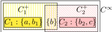
C1 : {a, b1} {b}C2: {b2, c}
C2+
C1+ C∞
Figure 13. Two source cliques from the graph in Figure 11, their saturations, and their enclosing clique C∞ in G∞.
5.3. Shortcut results. In order to establish short-cut results for our summaries, we start by investi-gating how property cliques are impacted by satu-ration.
In G∞, every G node has all the data properties it had in G, therefore two data properties belong-ing to a G clique are also in the same clique of G∞. Further, if the schema of G comprises subProperty constraints, a node may have in G∞a data property that it did not have in G. As a consequence, each G∞ clique includes one or several cliques from G, which may “fuse” by acquiring more properties due to saturation with subProperty constraints. An ex-ample is given in Figure 13, where C1+ and C2+ are the saturations of the source cliques C1, C2, while
C∞= {a, b1, b, b2, c} is a source clique of the graph
G∞(also in Figure 11).
Based on Theorem 2 and the above observations, we show:
Theorem 3. (W shortcut) The shortcut holds for ≡W.
For instance, on the graph in Figure 11, it is easy to check that applying summarization on (G/W)∞(as
prescribed by the shortcut) leads exactly to a graph strongly isomorphic to (G∞)/W.
Showing Theorem 3 is rather involved; we do it in several steps. First, based on a technical Lemma (see Appendix E) , we show:
Lemma 1. (Property relatedness in W sum-maries) Data properties are target-related (resp. source-related) in (G/W)∞ iff they are target-related
(resp. source-related) in G∞.
Based on the above Lemma and Theorem 1, we establish the next result from which Theorem 3 di-rectly follows:
Proposition 3. (Same cliques-W) G∞ and
(G/W)∞have identical source clique sets, and
identi-cal target cliques sets. Further, a node n ∈ G∞ has exactly the same source and target clique as fW(n)
in (G/W)∞.
Theorem 4. (S shortcut) The shortcut holds for ≡S.
We prove this based on counterparts of state-ments established for G/W. First we show:
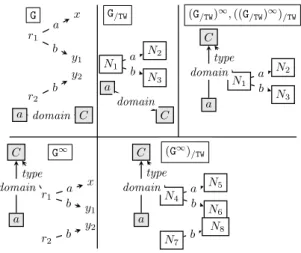
y2 y1 x r1 a b r2 b a domain C G N1 N2 N3 a b G/TW a C domain N1 N2 N3 a b C type (G/TW)∞, ((G/TW)∞)/TW a domain r1 x y1 a b C type G∞ r2 y2 b a domain N4 N5 N6 a b C type (G∞) /TW N7 N8 b a domain
Figure 14. Shortcut counter-example.
Lemma 2. (Property relatedness in S sum-maries) Data properties are target-related (resp. source-related) in (G/S)∞ iff they are target-related
(resp. source-related) in G∞.
Then, from Theorem 1 and the above Lemma, we obtain the next proposition from which Theorem 4 directly follows:
Proposition 4. (Same cliques-S) G∞ and
(G/S)∞ have identical source clique sets, and
iden-tical target clique sets. Further, a node n ∈ (G/S)∞
has exactly the same source and target clique as fS(n) in (G/S)∞.
Finally, we have:
Theorem 5. (No shortcut for ≡TW) The
short-cut does not hold for ≡TW.
We prove this by exhibiting in Figure 14 a counter-example. In G and G/TW, all data nodes are
untyped; only after saturation a node gains the type C. Thus, in G/TW, one (untyped) node represents all
data property subjects; this is exactly a “hasty fu-sion” as discussed below Theorem 2. In (G/TW)∞,
this node gains a type, and in ((G/TW)∞)/TW, it is
represented by a single node. In contrast, in G∞, r1
is typed and r2isn’t, leading to two distinct nodes
in (G∞)/TW. This is not strongly isomorphic with (G/TW)∞which, in this example, is strongly
isomor-phic to ((G/TW)∞)/TW. Thus, the shortcut does not
hold for ≡TW.
Theorem 6. (No shortcut for ≡TS) The
short-cut does not hold for ≡TS.
The graph in Figure 14 is also a shortcut counter-example for TS.
Based on Theorem 2, we have also established: Theorem 7. (Bisimilarity shortcut) The shortcut holds for the forward (≡fw), backward (≡bw), and forward-and-backward (≡fb) bisimilar-ity equivalence relations (recalled in Section 2.2).
G/fb G/S G/W (G/fb)∞ (G/S)∞ (G/W)∞ ∞ ∞ ∞ /W /S G /fb /S /W (G∞) /W (G∞)/S (G∞)/fb G∞ ∞ /fb /S /W /W /S /fb G/TW /TW G/TS /TS /TW /TS (G∞) /TW /TW (G∞) /TS /TS
Figure 15. Relations between quotient summaries.
5.4. Relationships between summaries. From the definition of weak and strong equivalence, it is easy to show that (G/S)/W= G/W, i.e., one could
com-pute G/W by first summarizing G into G/S, and then
applying weak summarization on this (typically much smaller) graph; similarly, (G/TS)/TW = G/TW.
It is also the case that (G/W)/S = G/W, i.e., strong
summarization cannot compress a weak summary further, and similarly (G/TW)/TS = G/TW. Figure 15
summarizes the main relationships between G, G∞, our summaries and bisimilarity-based ones.
6. From summaries to visualizations We now describe how to go from a quotient sum-mary to a graphical visualization such as the one illustrated in the Introduction.
6.1. Leaf and type inlining. For structurally simple graphs like our sample G shown in Fig-ure 2, quotient summaries have very few nodes and edges, and any node-link visualization method can be used. We explain here how we obtained our vi-sualizations, illustrated in our online gallery1.
To further simplify summaries, we apply leaf and type inlining, as follows. We remove type edges; in-stead, each type attached to a node in the summary is shown in the box corresponding to the node, after the node ID. Similarly, for each edge n−→ m wherea m is a leaf, we include a as an “attribute” of n, and do not render m (we say it has been “inlined” within n). A sizable part of an RDF graph’s nodes are leaves; as we will show, inlining them into their parent nodes greatly simplifies the visualization.
Figure 16 illustrates inlining for the S summary (Figure 9) of our sample graph. This summary is extremely compact, yet rich with information; pro-fessors, students, and courses are visible at a glance. Articles have been inlined within their authors as they were leaves in G/S. This simplification can also
be seen as a small loss of information: Figure 16 does not immediately suggest that Professors may have written articles together with GradStudents. However, (i) only leaf nodes are folded and (ii) af-ter a first glance, users may pursue exploration by other means (e.g., queries to check for such joint
Figure 16. Visualization result-ing from leaf and type inlinresult-ing on the sample Strong summary from Figure 9.
articles). Thus, we consider that inlining is overall beneficial, and systematically apply it on summaries before visualization.
If type-then-data summarization is used based on the most general types (Section 5.1), the most general types are shown at the top of each typed summary node (immediately under the node ID), then the actual types of the graph nodes represented by the summary node are shown one per line, under the most general types. N1, N7 and N8 in Figure 1 illustrate this.
6.2. Summary statistics. If users are interested (also) in a quantitative view of an RDF graph, our summaries can also plot a set of statistics. We de-scribe them below and illustrate them based on Fig-ure 1. For each summary node Ni, we display:
• The number of G nodes represented by Ni,
in parenthesis after “Ni” in the
correspond-ing box, e.g., “N8 (25000)”;
• For each type c such that x τ c for some x represented by Ni, the number of G nodes
represented by Ni which are of type c, e.g.,
http://db.uwaterloo.ca/~galuc/ wsdbm/ProductCategory0:807
• For each data property p such that (i) x p y for some x represented by Niand (ii) all the
objects of p triples whose subjects are rep-resented by Ni are leaves in G, the number
of such p triples, and the number of distinct targets of such triples. For instance, within N8, “bookedition (847 → 6)” denotes that there are 847 bookedition triples whose sub-jects are represented by N8, and they reach a total of 6 distinct objects (which are leaf nodes).
For each summary edge Ni a
−→ Nj where a is a
data property, the number of x a y triples in G such that x is represented by Ni and y is represented by
Nj. The label “hasGenre (58787)” on the edge from
N8 to N1 is an example of such an edge statistic. All these statistics can be gathered by our sum-mary construction algorithms (Section 7), at no ex-tra computational cost.
6.3. Visualizing very large summaries. For a very complex (e.g., encyclopedic) dataset, even the graph obtained from inlining may have too many
nodes and edges for an effective visualization. If it has several connected components (one per do-main), each of them can be viewed separately. Oth-erwise, it can be split into several, possibly over-lapping subgraphs, using any graph decomposi-tion strategy (for instance, minimize the number of times the representatives of two nodes connected in G appear in different summary subgraphs etc.) Information discovery in such graphs requires more computational and cognitive effort.
7. Summarization algorithms
We now present summarization algorithms which, given as input a graph G, construct G/W, G/S,
G/TWand G/TS. All our algorithms have an amortized
linear complexity in the size of G: they can be built in just one or two passes over the data. Our incre-mental algorithms, capable of reflecting additions to G, into its previously computed summaries, are the most involved.
7.1. Global data graph summarization. The first algorithms we present summarize only the data triples through two graph traversals: one to learn the equivalence relation7 and create the summary nodes, the second to determine the representative of each G node and, as a consequence, add triples to the summary.
We start with our global W summarization algorithm (Algorithm 1). It exploits Proposition 1, which guarantees that any data property occurs only once in the summary. To each data property p encoun-tered, it associates a summary node (integer) sp which will be the (unique) source of p in the sum-mary, and similarly a node tp target of p; these are
initially unknown, and evolve as G is traversed. Fur-ther, it uses two maps op and ip that associate to each data node n, the set of its outgoing, resp. in-coming data properties. These are filled during the first traversal of G (step 1.) Steps 2. to 2.5 ensure that for each node n having outgoing properties and possibly incoming ones, spfor all the outgoing ones
are equal, and equal also to tp for all the incoming
ones. This is performed using a function fuse which, given a set of summary nodes, picks one that will re-place all of them. In our implementation, summary nodes are assigned integer IDs, and fuse is simply min; we just need fuse to be distributive over ∪, i.e., fuse(A, (B ∪ C)) = fuse(fuse(A, B), fuse(A, C)). Symmetrically, step 3. ensures that the incom-ing properties of nodes lackincom-ing outgoincom-ing proper-ties (thus, absent from op) also have the same tar-get. In Step 4., we represent s and o based on the source/target of the property p connecting them.
7Our equivalence relations are defined based on the triples of a given graph G, thus when summarization starts, we do not know whether any two nodes are equivalent; the full equivalence relation is known only after inspecting all G triples.
global-W(G)
1. For each s p o ∈ G, add p to op(s) and to ip(o).
2. For each node n ∈ op:
2.1. Let X ← fuse{sp| p ∈ op(n)}.
If X is undefined, let X ←nextNode(); 2.2. Let Y ← fuse{tp| p ∈ ip(n)}.
If Y is undefined, let Y ←nextNode(); 2.3. Let Z ← fuse(X, Y );
2.4. For each p ∈ ip(n), let sp← Z;
2.5. For each p ∈ op(n), let tp← Z;
3. Repeat 2 to 2.5 swapping ip with op and tpwith sp;
4. For each s p o ∈ G: let fW(s) ← sp, fW(o) ←
tp;
Add fW(s) p fW(o) to G/W.
Algorithm 1: Global W summarization of a graph
The fuse operations in 2. and 3. have ensured that, while traversing G triples in 4., any data node n is always represented by the same summary node fW(n).
Our global S summarization algorithm (Algo-rithm 2) uses two maps sc and tc which store for each data node n, its source clique sc(n), and its target clique tc(n), and for each data property p, its source clique srcp and target clique trgp. Further, for each (source clique, target clique) pair encoun-tered during summarization, we store the (unique) corresponding summary node. Steps 1.-1.2. build the source and property cliques present in G and as-sociate them to every subject and object node (in sc and tc), as well as to any data property (in srcp
and trgp). For instance, on the sample graph in
Figure 2, these steps build the cliques in Table 2. Steps 2-2.2. represent the nodes and edges of G.
The correctness of algorithms global-W and global-S follows quite easily from their descriptions and the summary definitions.
7.2. Incremental data graph summarization. These algorithms are particularly suited for incre-mental summary maintenance: if new triples ∆+G are added to G, it suffices to summarize only ∆+G, based on G/≡and its representation function f≡, in
order to obtain (G ∪ ∆+G)/≡. Incremental algorithms
are considerably more complex, since various deci-sions (assigning sources/targets to properties in W, source/target cliques in S, node representatives in both) must be repeatedly revisited to reflect newly acquired information about G triples, as we shall see.
Each incremental summarization algorithm con-sists of an incremental update method, called for ev-ery data triple, which adjusts the summary’s data structures, so that at any point, the summary re-flects exactly the graph triples visited until then.
global-S(G)
1. For each s p o ∈ G:
1.1. Check if srcp, trgp, sc(s) and tc(o) are
known; those not known are initialized with {p};
1.2. If sc(s) 6= srcp, fuse them into new
clique src0p= sc(s) ∪ srcp; similarly, if tc(o) 6=
trgp, fuse them into trgp0 = tc(o) ∪ trgp. 2. For
each s p o ∈ G:
2.1. fS(s) ← the (unique) summary node
corresponding to the cliques (sc(s), tc(s)); similarly, fS(o) ← the node corresponding to
(sc(o), tc(o)) (create the nodes if needed). 2.2 Add fS(s) p fS(o) to G/S.
Algorithm 2: Global S summarization of a graph
increm-W(s p o)
1. Check if spand op are known: either both
are known (if a triple with property p has al-ready been traversed), or none;
2. Check if fW(s) and fW(o) are known; none,
one, or both may be, depending on whether s, respectively o have been previously encoun-tered;
3. Fuse sp with fW(s) (if one is unknown,
as-sign it the value of the other), and op with
fW(o);
4. Update fW(s) and fW(o), if needed;
5. Add the edge fW(s) p fW(o) to G/W.
Algorithm 3: Incremental W summarization of one triple
Algorithm 3 outlines incremental W summariza-tion. For example (see the figure below), let’s as-sume the algorithm traverses the graph G in Figure 2 starting with: p1advises p2, then p1wrote a1, then
p4teaches c2. When we summarize this third triple,
we do not know yet that p1 is equivalent to p4,
be-cause no common source of teaches and advises (e.g., p3 or p4) has been seen so far. Thus, p4 is
found not equivalent to any node visited so far, and represented separately from p1. Now assume
the fourth triple traversed is p4 advises p5: at this
point, we know that advises, wrote and teaches are in the same source clique, thus p1 ≡W p4, and
their representatives (highlighted in yellow) must be fused in the summary (Step 3.) More generally, it can be shown that ≡Wonly grows as more triples are visited, in other words: if in a subset G0 of G’s triples, two nodes n1, n2are weakly equivalent, then
![Figure 5. ∼ ioa summary [5] of the RDF graph in Figure 2.](https://thumb-eu.123doks.com/thumbv2/123doknet/12271845.321710/7.892.451.788.110.483/figure-ioa-summary-rdf-graph-figure.webp)