HAL Id: hal-00864258
https://hal.archives-ouvertes.fr/hal-00864258
Submitted on 20 Sep 2013
HAL is a multi-disciplinary open access
archive for the deposit and dissemination of
sci-entific research documents, whether they are
pub-lished or not. The documents may come from
teaching and research institutions in France or
abroad, or from public or private research centers.
L’archive ouverte pluridisciplinaire HAL, est
destinée au dépôt et à la diffusion de documents
scientifiques de niveau recherche, publiés ou non,
émanant des établissements d’enseignement et de
recherche français ou étrangers, des laboratoires
publics ou privés.
Relocation of Mobile Wireless Sensors in the Presence of
Obstacles
Saoucene Mahfoudh, Ines Khoufi, Pascale Minet, Anis Laouiti
To cite this version:
Saoucene Mahfoudh, Ines Khoufi, Pascale Minet, Anis Laouiti. Relocation of Mobile Wireless Sensors
in the Presence of Obstacles. ICT 2013 - 20th International Conference on Telecommunications, May
2013, Casablanca, Morocco. pp.1-5. �hal-00864258�
Relocation of Mobile Wireless Sensors in the
Presence of Obstacles
Saoucene Mahfoudh
∗, Ines Khoufi
†, Pascale Minet
‡, Anis Laouiti
§∗saoucene.ridene@inria.fr,†ines.khoufi@inria.fr, ‡pascale.minet@inria.fr,§anis.laouiti@it-sudparis.eu ∗†‡INRIA, Rocquencourt, 78153 Le Chesnay Cedex, France
§TELECOM SudParis, CNRS Samovar, UMR 5157, France
Abstract—In many applications (e.g military, environment monitoring), wireless sensors are randomly deployed in a given area. Unfortunately, this deployment is not efficient enough to ensure area coverage and network connectivity. Algorithms based on Virtual Forces are used to improve the random initial deployment. In this paper, we want to ensure coverage and network connectivity in a given area containing obstacles. We enhance the Distributed Virtual Forces Algorithm (DVFA) to cope with obstacles. Obstacles are characterized by prohibiting both the physical presence of sensors and the wireless communication. Performance evaluation shows that DVFA provides an efficient deployment even if obstacles exist in the considered area.
I. MOTIVATION
Wireless Sensor Networks (WSNs) have a large potential for numerous application areas like military, medical, environ-mental and industrial. A WSN is a collection of autonomous wireless nodes scattered in an area of interest. Each node has a sensing range to measure parameters of its enviromnent and a communication range to maintain connectivity with other nodes. Many research works in WSNs are interested in the deployment of sensors that ensure both coverage and network connectivity. Random deployment is simple but it is source of several problems. Indeed, we can obtain many disconnected islands and some regions can be densely covered whereas others are weakly covered.
Our objective is to redeploy wireless sensors to achieve the full area coverage and the connectivity between all sensors. In a real environment, obstacles such as trees, walls and buildings may exist and impact the deployment of wireless sensors. In fact, obstacles can prohibit the network connectiv-ity between nodes and create some uncovered holes or some accumulation of sensors in the same region. Consequently, an efficient wireless sensors deployment algorithm is required to ensure both coverage and network connectivity in the presence of obstacles.
In this paper, we focus on this problem and propose the Distributed Virtual Force Algorithm (DVFA) [5] to redeploy wireless sensors in an area where obstacles exist.
II. STATE OF THE ART
A. Decentralized network deployment
In a decentralized configuration, mobile sensors organize themselves dynamically to cover a given area. They need to be autonomous, where their movement is self-controlled based on local knowledge only. This knowledge is usually
collected from their neighborhood by means of control mes-sage exchange. A control mesmes-sage contains data such as the identification of a sensor node, its position, its speed, its residual energy. It might also include the list of its neighbors. Most of the decentralized algorithms found in the litterature [1], [3], [2], [4], rely on the principle of the forces exerted between different nodes within the sensor network.
Each pair of sensor nodes that are close enough exerts on each other repulsive or attrative forces. The intensity of the force is function of the distance between the two sensor nodes. The sensor node movement (distance to travel, direction, speed) will be then dictated by the sum of all the forces exerted on it by its neighbors. Obviously, if the sum of the forces is null the sensor node does not move. This calculation process must be run by every mobile sensor node separately and continuously as long as the node is still under the pressure of its neighbors. Nodes should stop moving once they reach a stable position, in other words a position where the sum of the exerted forces tends to zero.
In the distributed configurations, sensor nodes having dy-namic and partial network knowledge must collaborate to accomplish a same common mission (e.g. achieve maximum coverage of an area, or deployment around a specified center of interest). All the nodes must use the same strategy, as well as the same set of parameters that must be tuned in order to accelerate the convergence of the distributed algorithm and avoid possible oscillations. And of course because of the energy constraints of this kind of autonomous devices, the model should minimize the travelled distance of each node before it reaches its stable position.
B. Network deployment with obstacles
Obstacles such as walls or buildings might exist in the environment where sensors are deployed. Obstacles have two major features:
• Obstacle prohibits any physical presence of sensor. Any mobile sensor cannot cross obstacle but it can only move along the boundary. Then, the obstacle’s area is empty of sensors.
• Obstacle can prohibit wireless sensor communication. If
the line of sight between two sensors goes through the ob-stacle then the direct communication between them may be impossible. For a more detailed study of obstacles, see [14].
The presence of obstacles might cause the disruption of wireless sensor communications. Consequently, ensuring area coverage and network connectivity becomes a more complicated task.
With regard to the existing sensor deployment strategies to ensure coverage in the presence of obstacles we adopt the classification proposed by [6], namely grid based, computational geometry based and force based strategies illustrated in Figure 1.
In the grid based approach, sensors will redeploy according to a predetermined grid: triangular lattice, square or hexagonal grid (an example of square grid and hexagonal grid is illustrated in Figure 1a and 1b respectively). The triangular lattice is preferred because it requires the smallest number of sensors to achieve coverage [7]. The grid size depends on network density. Grid can be used in robotic where robot moves according to defined rules (generally along grid lines) and deploys sensors to achieve the full coverage of the considered area. To reach this goal, different strategies are proposed (spiral trajectory [8], serpentine trajectory [9], go back [10] or clockwise move around the obstacle [8]..) to define the trajectory of the robot in the given area taking into account the presence of obstacle modeled as a simple polygon of finite size.
The computational geometry based approach uses the Voronoi diagram and the Delaunay triangulation (see Figure1c). In [12], authors designed a deterministic coverage method to find the uncovered holes and place sensors efficiently for both obstacles and regions.
The virtual force based approach is based on virtual forces to move sensors. Each sensor node exerts an attractive or repulsive force on each neighboring sensor according to the distance between them in order to reach the target distance, where no force is exerted (see Figure 1d). Considering arbitrary communication range and sensing range, CPFV [11] (Connectivity-Preserved Virtual Force) is an enhanced scheme for the traditional virtual force method that guarantees network connectivity and tries to maximize the coverage ratio. This scheme divides the area into floors of common height, twice the sensing range then sensors try to stay at the central floor lines. While connectivity is guaranteed, this scheme reduces the overlaps of sensing range and then improves the global network coverage. Young and al [13] propose to apply three virtual forces: Fcoverto maximize the coverage, Fdegree
to keep the number of neighboring sensors at the degree k and Fobstacleto avoid obstacle. These authors also propose to
use the virtual force Fdamper to stop the mobile sensor from
continuous movement. These new virtual forces guide the mobile sensor to maintain connectivity, maximize coverage and avoid obstacles in a given area.
In this work, we propose the Distributed Virtual Force Algorithm to deploy mobile wireless sensors in an area containing obstacles in order to ensure coverage and connectivity.
a Square grid b Hexagonal grid c Voronoi diagram
d Virtual forces
Fig. 1: Coverage strategies
III. DISTRIBUTEDVIRTUALFORCESALGORITHM
A. DVFA principles
Distributed Virtual Forces Algorithm (DVFA) is designed in order to redeploy wireless sensors to ensure area coverage and network connectivity.
In this paper we assume the condition R ≥ 2r where R is the communication range and r is the sensing range of any sensor. This condition guarantees the network connectivity when the full coverage is ensured.
Starting from a random deployment that may produce scattered islands of connected sensors, DVFA tries to discover them and fusion them to ensure the coverage purpose. This is possible by sensors moves. Sensors moves are handled by the virtual forces principle.
DVFA is based on a periodic exchange of Hello messages between sensors. It assumes that any sensor node knows its position (e.g using a GPS). These Hello messages enable wireless sensor nodes to detect the arrival and departure of sensors in the vicinity. The Hello message informs sensors about the position of the sender as well as the list of its 1-hop neighbors. Then, at each iteration, each sensor can compute the forces exerted on it by neighbor sensors until 2-hop neighbors [5]. Let us consider two sensor nodes siand sj. Let dij be the
distance between them and Dthbe the target distance between
two neighbor sensors. Dthcan be obtained by computing the
distance between two neighbors in the optimal deployment using hexagons illustrated in Figure 1b. The force exerted by sj on si is: • Attractive if dij > Dth. We have −→ Fij = Ka(dij − Dth) (xj−xi,yj−yi) dij , where Ka is a coefficient in [0, 1); • Repulsive if dij < Dth. We have −→ Fij = Kr(Dth − dij) (xj−xi,yj−yi) dij , where Kr is a coefficient in [0, 1);
• Null if dij = Dth.
The resulting force exerted on si is equal to
− → Fi=P −
→ Fij.
The new position of sensor siwhose current position is (xi, yi)
is given by (x0i, yi0) with x0i = xi+ x-coordinate of
− → Fi and y0i = yi+y-coordinate of − →
Fi. The distance traveled at each
iteration, to reach this new position can never exceed a fixed threshold Lmax. Lmax enables to save energy by reducing oscillations in sensor moves. The Hello period must be larger than the time needed to compute DVFA and to travel the distance Lmax.
Before moving to the new position, sensor sends a Bye message including its position after its next move to enable the neighboring sensors to update their neighborhood tables and compute a more accurate value of the virtual forces exerted on them. Finally, the node moves to its new position. A new iteration starts.
B. DVFA with obstacles
Obstacles can exist in a given area and cause an inefficient deployment as it blocks any physical presence of sensors and may prevent the communication between neighboring sensors. In this work, we propose to extend DVFA to cope with obstacles in 2D. We assume that any sensor is able to detect the shape and position of any obstacle at a distance less than or equal to Lmax. We also assume that any obstacle is modeled by one rec tangular block or a juxtapostion of rectangular blocks. In this paper, we consider obstacles of various shapes: U , Z and L (See Figures 6, 9 and 11). Each node si computes the resulting force
− → Fi using
DVFA and deduces its new position. If it detects an obstacle between its current position and its new one, it recomputes its new position taking into account the presence of the obstacle that exerts a repulsive force to prevent its penetration. Figure 2 shows the force exerted by the obstacle on the node which computes its final position. We notice that the repulsive force exerted by the obstacle depends on the force −→Fi.
Fig. 2: The force exerted by the obstacle to compute node’s final position
If the new position of node computed by DVFA exceeds the obstacle, we distinguish two strategies to compute its final position:
• Strategy S1 blocks the sensor node whatever its new
position. The force exerted by the obstacle is such that
it cancels the projection of the resulting force −→Fi on the
axis orthogonal to the closest edge of the obstacle (see Figure 3). Hence, the mobile sensor moves in parallel to the edge of the obstacle.
Fig. 3: Strategy S1
• Strategy S2 blocks the sensor node only if the new
position of the sensor is within the obstacle as it is shown in Figure 2. In this case, the force exerted by the obstacle is similar to the force used in strategy S1. Otherwise, the
sensor moves around the obstacle to its new position (see Figure 4).
Fig. 4: Strategy S2
IV. PERFORMANCE EVALUATION
We have implemented the DVFA protocol as an agent in the NS2 simulator and have performed simulations for different wireless sensor networks taking into account various shapes and positions of obstacles. Simulation parameters are given in the following Table I. Using these parameters, we compute the value of Dth in the optimal hexagonal deployment. The
obtained value is Dth= 43.3m. The value of Ka and Kr are
close to those used in the literature. A. Evaluation criteria
The goal of DVFA is to obtain the maximum coverage with the redeployment of network nodes. To compute the coverage rate, we divide the network area into 500x500 unit grids. A grid is considered covered if and only if its centered point is covered by at least one sensor node. In this performance study, we will evaluate the coverage rate as a function of time in various configurations. We compare the performance results of DVFA with and without obstacles, considering different obstacles shapes and different strategies to cope with the obstacles.
TABLE I: Simulation parameters
Topology
Sensor nodes 200 randomly distributed in 2 islands of communication Sensor speed 10 m/s
Sensing range 25 m Considered area 500m x 500m Simulation
Result average of 10 simulation runs Simulation time 250s MAC Protocol IEEE 802.11b Throughput 2 Mb/s Communication range 50 m DVFA
Ka 0.001 see section III.A Kr 0.56 see section III.A Hello period 1.0 s see section III.A
B. Simulation results
An example of initial deployment is represented in Figure 5 where wireless nodes are grouped in two islands of commu-nication located at the top left and bottom right of the area.
Fig. 5: Initial deployment
Fig. 6: DVFA redeployment
Figure 6 illustrates the final deployment in the presence of a Z obstacle where the target distance between two neighbors is Dth. Figure 7 shows the evolution of the coverage rate
with time using strategy S1. DVFA with obstacles reaches a
coverage rate as good as DVFA without obstacles. Indeed, after a time of 200s (of simulated real time) the coverage rate is about 99%. These good results can be explained by the repulsive force exerted by the obstacle that obliges sensors to move along the edge of the obstacle.
Fig. 7: Coverage rate with and without obstacles In the second series of experiments, we compare the two strategies S1 and S2 for the same Z obstacle. Results are
illustrated in Figure 8. Both strategies give close coverage rates. However, strategy S2 is more realistic and easier to
implement. Strategy S1requires a moving pattern to go around
the obstacle. The distance traveled by sensors may increase significantly according to the obtacle’s shape.
Fig. 8: Coverage rate with strategies S1 and S2
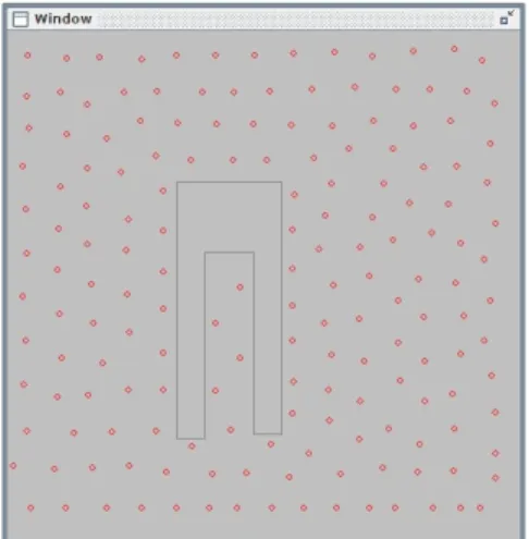
Considering the initial deployment depicted in Figure 5, we study the impact of the shape of the obstacle on the coverage rate. Figure 9 illustrates the final deployment with an U obstacle. Figure 10 compares the evolution of the coverage rate for U obstacle and Z obstacle. It appears that the coverage is slightly smaller with the U obstacle than the Z obstacle (2%). This is due to the confined area in the U shape. The U obstacles require more time to improve the coverage.
Fig. 9: Final deployment with an U obstacle
Fig. 10: Coverage rate with Z obstacle and U obstacle
In the fourth series of experiments, we consider an obstacle of shape L, as illustrated by Figure 11. The coverage rate is very closed to the one obtained with the Z obstacle in Figure 7.
Fig. 11: Final deployment with an L obstacle V. CONCLUSION
In this paper, we enhance DVFA to cope with obstacles. Our idea is to keep the simplicity of the DVFA algorithm to ensure the full coverage and network connectivity in the presence of obstacles. To achieve this, we add a repulsive force
exerted by the obstacle on any node whose new position goes through or penetrates the obstacle. Consequently, at the end of deployment, no mobile sensor node is within the obstacle. We have studied two different strategies to ensure coverage in an area containing obstacles. Both of them exhibit similar coverage rates. However strategy S1 is more realistic and
easier to implement. Strategy S2 requires a moving pattern
to allow sensor to reach its new position beyond the obstacle. Moreover, we have performed several series of experiments with different obstacle shapes. Results show that the coverage rate depends on the obstacle shape. U shape requires more time than Z shape or L shape to ensure coverage of the considered area. As a further work, we will see how to relax the condition binding the communication range and the sensing range of sensors while maintainig connectivity and maximizing coverage.
REFERENCES
[1] N. Heo, P. K. Varshney, ”A distributed self spreading algorithm for mobile wireless sensor networks”, 2003 IEEE In Wireless Communications and Networking (WCNC 2003). 2003 IEEE, Vol. 3 (2003), pp. 1597-1602 vol.3. New Orleans, LA, USA.
[2] A. Howard, M.J. Mataric, G. Sukhatme, ”Relaxation on a mesh: a formal-ism for generalized localization”, International Conference on Intelligent Robots and Systems, (IROS 2001), Wailea, Hawaii, USA.
[3] C. Safak Sahin, E. Urrea, M. Umit Uyar, M. Conner, G. Bertoli, C. Pizzo,”Design of genetic algorithms for topology control of unmanned vehicles”, International Journal of Applied Decision Sciences 2010 - Vol. 3, No.3 pp. 221 - 238.
[4] M. Garetto, M. Gribaudo, C.F. Chisserini and E. Leonardi, ”Sensor de-ployment and relocation: a unified scheme”, Journal of Computer Science and Technology, 2008.
[5] K. Mougou, S. Mahfoudh, P. Minet, A. Louiti ”Redeployment of Ran-domly Deployed Wireless Mobile Sensor Nodes” IEEE VTC2012, Quebec, Canada, September 2012.
[6] N. A. Ab. Aziz, K. Ad. Aziz and Z. W. Ismail ”Coverage startegies for wireless Sensor Networks” World academy of science, Engineering and technology 50 2009.On the
[7] K. Xu G. Takahara and H. Hassanein ”Robustness of Grid-based Deploy-ment in Wireless Sensor Networks” IWCMC 2006, Canada.
[8] C. Y. Chang, J. P. Sheu, Y. C. Chen, S. W. Chang, ”An Obstacle-Free and Power-Efficient Deployment Algorithm for Wireless Sensor Networks” IEEE Transaction on systems, man, and cybernetics, vol.39, no. 4, Jul 2009. [9] C. Y. Chang, C. T. Chang, Y. C. Chen, H. R. Chang, ”Obstacle-Resistance Deployment Algorithm for Wireless Sensor Networks” IEEE Transaction on vehicular technology, vol.58, no. 6, Jul 2009.
[10] C. Y. Chang, C. T. Chang, C. Y. Hsieh, C. C. Chen, Y. C. Chen, ”A Dead-End Free Deployment Algorithm for wireless Sensor Networks with Obstacles” in Proc. IWCMC, 2010, pp.84-88.
[11] G. Tan, S. A. Jarvis, A. M. Kermarrec, ”Connectivity-Guaranteed and Obstacle-Adaptive Deployment Schemes for Mobile Sensor Networks” IEEE Transactions on Mobile Computing (2009).
[12] T. Haisheng, W. Yuexuan, H. Xiaohong, H. Qiang-Sheng, C. M. L. Francis, ”Arbitrary Obstacles Constrained full Covrage in Wireless Sensor Networks,” WASA , 2010, pp. 1-10.
[13] Y. S. Jeong, Y. H. Han, J. J. Park, S. Y. Lee ”MSMS: mobile sensor network simulator for area coverage and obstacle avoidance based on GML” EURASIP journal on Wireless Communication and Networking 2012.
[14] J. M. Gorce, K. Jaffres-Runser and G. De La Roche, ”The Adaptive Multi-Resolution Frequency-Domain ParFlow (MR-FDPF) Method for In-door Radio Wave Propagation Simulation. Part I : Theory and Algorithms,” Inria RR 5740, May 2006.