Relative efficiency of non parametric error rate estimators in multi-group linear discriminant analysis

African Journal of Mathematics and Computer Science Research Vol. 2(10), pp. 218-224, November, 2009 Available online at http://www.academicjournals.org/AJMCSR ISSN 2006-9731

© 2009 Academic Journals

Full Length Research Paper

Relative efficiency of non parametric error rate

estimators in multi-group linear discriminant analysis

Romain Lucas Glèlè Kakaï

1

*, Dieter Pelz

2

and Rudy Palm

3

1_{Faculty of Agronomic sciences, University of Abomey-Calavi, 04 BP 1525, Cotonou, Benin.} 2_{Department of Forest Biometry, University of Freiburg, Germany.}

3_{Gembloux Agricultural University, Passage des Déportés 2. B-5030 Gembloux Belgium.}

Accepted 1 September, 2009

A Monte Carlo study was achieved to assess the relative efficiency of ten non parametric error rate estimators in 2, 3 and 5-group linear discriminant analysis. The simulation design took into account the number

p

of variables (4, 6, 10, 18) together wit the size sample

n

so that:

n/

p

= 1.5, 2.5 and 5. Three values of the overlap, e of the populations were considered (e=0.05, e=0.1, e=0.15) and their common distribution was Normal, Chi-square with 12, 8, and 4 df; the heteroscedasticity degree,

Γ

was measured by the value of the power function, 1- of the homoscedasticity test related to

Γ

(1- =0.05, 1- =0.4, 1- =0.6, 1- =0.8). For each combination of these factors, the actual error rate was empirically computed as well as the ten estimators. The efficiency parameter of the estimators was their relative error, bias and efficiency with regard to the actual error rate, empirically computed. The results showed the overall best performance e632 estimator. On the contrary,

e

0

,

epp

,

eppCV

and

eA

recorded the lowest performance in terms of mean relative error and mean relative bias. The ranks of the estimators were not influenced by the number of groups but for high values of the later, the mean relative bias of the estimators tend to zero.

Key words: Error rate, estimation, efficiency, multi-group, linear rule, simulation. INTRODUCTION

Discriminant analysis is a statistical method of allocation of unknown individual to one group, from at least two foreknown groups, by using a classification rule previously established on well-known individuals. A number of classification rules are available and the most used are linear, quadratic and logistic methods.

Many classification rules have been proposed in literature and the most common is the linear classification rule (Fisher, 1936).

Let’s suppose g p-variate populations

P

_k

(

k

=

1

,...,

g

)

, with mean vectors, k

(

k

=

1

,...,

g

)

and common covariance matrices, . The linear rule (

LR

) is a

*Corresponding author. E-mail: gleleromain@yahoo.fr. Tél: (00229) 95 84 08 00, (00229)90987810/97399077. Fax: (00229) 21 30 30 84.

Normal-based classification rule for which

F

=

N(

k

,

)

(McLachlan, 1992):

(

,

N(

,

)

)

LR

x

i k =

ln(

p

k

/

p

l

)

+

(

0

.

5

(

)

)

' 1

(

)

l k l k i

−

+

−

−

x

; (1.1)

)

;

,...

1

,

(

k

l

=

g

k

≠

l

The unknown observation vector

x

i is assign to

G

k if:

(

,

N(

,

)

)

LR

x

i k

≤

0

∀

l

=

1

,...,

g

;

l

≠

k

. In the case of data samples, LR can be established by replacing in (1.1) the parameters, k

(

k

=

1

,...,

g

)

and by their estimates,

ˆ

k

(

k

=

1

,...,

g

)

and

ˆ

k;

ˆ

is consi-

dered in (1.1) as the estimated pooled covariance matrix of the k populations.

Whatever the rule established is, it is subject to a probability of misclassifications. Then, an actual error rate is associated with any classification rule established on data samples in order to evaluate its efficiency. In practice, it is impossible to precisely determine the actual error rate, because it is only computed on the actual parameters of the populations, which are usually unknown. To solve this problem, some parametric and non parametric estimators of the actual error rate were established (McLachlan, 1992). Parametric estimators were established for two normal homoscedastic groups and estimated the actual error rate, using some para-meters related to the considered samples such as the estimated Mahalanobis distance between the two groups. On the contrary, non-parametric error rate estimators do not depend on any hypothesis of use and were based on resampling methods. For two-group discriminant analysis, many comparison studies of error rate esti-mators have been done in linear discriminant analysis, in order to deduce the ones that have the lowest errors compared with the theoretical actual error rate. A thorough review of these studies was provided by Schiavo and Hand (2000). However, in real world problems, more than two groups are often considered in discriminant analysis. This paper evaluated and com-pared by simulation technique, the efficiency of ten non parametric error rate estimators for 2, 3 and 5 groups submitted to linear discriminant analysis.

Actual error rate

The actual error rate can be defined as the theoretical proportion of misclassified observations, obtained by validating a classification rule established on data samples to any other observation taken from the same populations. This error rate is useful in practice because it gives the expected misclassification rate when a previously established rule is used.

Let’s assume two samples, E1 and E2 with

p

varia-bles and common size

n

. The mean vectors and the pooled covariance matrix are

x

₁ ,

x

₂ and

S

, respectively. Let’s also suppose that these samples are taken from normal populations, P1 and P2, with mean

vector _k(

k

=1, 2). The actual error rate specific to the group

k

,

ec

_k (

k

=1, 2) and the overall actual error rate are given by McLachlan (1975):

[

]

−

−

−

′

+

−

−

Φ

=

− − −

)

(

)'

(

)

(

)

(

2

1

)

1

(

2 1 1 2 1 2 1 1

x

x

S

S

x

x

x

x

S

x

x

1 k 1 2 k k

ec

and Kakaï et al. 219 =

=

2 1 k k k

ec

p

ec

, (2.1)

where

p

_k and

Φ

are respectively, the prior probability related to the group

k

and the cumulative function of the Normal distribution.

The relations (2.1) can only be used in two-group discriminant analysis when the linear rule is established on two normal homoscedastic populations. In the other cases, the actual error rate associated with a classi-fication rule can be empirically computed, for two groups, by determining the proportion of misclassified obser-vations when the rule is established on the samples E1

and E2 and validated on a couple of large samples, of

size 10,000 for example.

Estimation of the actual error rate

For more than two groups submitted to discriminant analysis, only non parametric estimators can be used to assess the actual error rate associated with an established rule; parametric estimators were only conceived for two-group discriminant analysis. Ten non-parametric error rate estimators were considered in the study and presented below.

Resubstitution estimator,

eA

(Smith, 1947): that is, proportion of misclassified observations when the rule was established and validated on the same samples.

Cross validation estimator,

eCV

(Lachenbruch, 1967): that is, proportion of misclassified observations when

gn

discriminant analyses were done on

gn

-1 observations by removing, at each step, one observation and by allocating the removed observation to one of the considered groups on the basis of the rule established on the

gn

-1 observations.

1

eS

and

eS

₂ Estimators (Hand, 1986):

eCV

n

n

eS

1

=

₂

2

₊

₁

and

eS

2

=

₂

2

_n

₊

n

₃

eCV

. (3.1)

epp

Estimator (Fukunaga and Kessell, 1972):

(

)

=

−

=

gn i i g i

gn

epp

1 1

)

(

),...,

(

ˆ

max

1

1

x

x

. (3.2)

The symbols

ˆ

_k

(

x

_i

)

(

k

=

1

,...,

g

) represented the posterior probability that an individual

i

, of observations

220 Afr. J. Math. Comput. Sci. Res. vector

x

i belongs to

G

k: =

=

g l l i i k i k

f

f

1

)

(

ˆ

/

)

(

ˆ

)

(

ˆ

x

x

x

;

)

(

ˆ

i k

f

x

was the value of the estimated density function at

x

i for population

G

k.

eppCV

Estimator (Fukunaga and Kessell, 1972): that is, computed by using the relation (3.2) in which the posterior probabilities,

ˆ

_k

(

x

_i

)

(

k

=

1

,...,

g

) of the observations vector

x

i was determined, using the classification rule established on

gn

-1 observations, the vector

x

i , being removed. Jackknife estimator,

eJc

(Quenouille, 1949): that is, computed by realising

gn

discriminant analyses on

gn

-1 observations. For each sample of

gn

-1 observations, the observation

i

being removed, the resubstitution estimator,

eA

_k(i) , specific to

G

_k (

k

=

1

,...,

g

), was computed. By assuming

k

A

e

, the means of

eA

_k(i): =

=

n i ki k

_n

eA

A

e

1 ()

1

_{; (3.3)} The Jackknife estimator is computed as:

(

+

−

−

)

=

= g k k k k

n

eA

e

A

eA

g

eJc

1

)

)(

1

(

1

, (3.4)

eA

_k being the resubstitution estimators specific to

G

_k and computed from the overall sample.

Ordinary bootstrap estimator,

eboot

(Efron, 1983): that is, computed on 100 bootstrap samples, a sample of size

n

being taken with replacement in each initial sample of size

n

. For each bootstrap sample, the classification rule was established and the resubstitution estimator,

eA

_kj* (k=1,...,g; j=1,...,100) specific to

G

_k was computed. The same rule was also used to compute the proportions,

*

k

r

of misclassified observations, the rule being validated on the initial sample. The bias,

b

_k

(

k

=

1

,...,

g

)

of

eA

_kj* was computed as follows:

=

−

=

100 1 * *

₎

(

100

1

j kj k k

eA

r

b

. (3.5)

The overall bootstrap estimator was computed as:

(

)

=

−

=

g k k k

b

eA

g

eboot

1

1

, (3.6) k

eA

being the resubstitution estimator specific to

G

_k

when the rule was established on the

gn

initial observations.

0

e

Estimator (Chatterjee and Chatterjee, 1983): that is, computed on 100 bootstrap samples,

t

*_i

(

i

=

1

,...,

100

)

_, taken from the initial sample

t

. For each bootstrap sam-ple, a classification rule is established and the proportion of misclassified observations of

t

, which do not belong to

*

t

i, was computed. The

e

0

estimator is the mean of the 100 proportions.

632

e

Estimator (Efron, 1983): that is, computed as follows:

0

632

.

0

368

.

0

632

eA

e

e

=

+

(3.7) SIMULATION DESIGN Discriminant model

We consider the case of 2, 3 and 5 groups submitted to linear discriminant analysis and characterized by their means and covariances matrices. In the case of 2 groups, the mean vector,

m

_k(

k

=1, 2) was so that:

1

m

= 0 ;

m

₂ =

(m

,

0

,...,

0

)'

; m ∈ IR+_.

The covariance matrix, _k (

k

=1, 2), was a diagonal matrix with

v

_k(

k

=1, 2), the vector of diagonal elements so that:

1

v

=

v

(

1

) ;

v

₂ =

v

(

) where

∈

IR+ and

(

v

)=

(

,

1

,...,

1

)'

In the case of 3 and 5 groups, the mean vectors,

m

_k and covariance matrices, _k were given below:

m1= 0 ; m2 =

(m

,

0

,...,

0

)'

; m3 =

( m

0

,

,

0

...,

0

)'

;

v

1 =

1

(

v

) ;

v

₂=

v

₃=

v

(

). For 5 groups: m1= 0; m2 =

(m

,

0

,...,

0

)'

; m3 =

( m

0

,

,

0

...,

0

)'

; m4 =

)'

0

,...

0

,

( m

−

; m5 =

(

0

,

−

m

,

0

,...,

0

)'

. 1

v

=

v

(

1

) ;

v

₂=

v

₃=

v

₄=

v

₅=

v

(

).

It was known that the linear rule is invariant under a non singular linear transformation (McLachlan, 1992). So, appropriate linear transformations applied to the simple models proposed above, will help to extend the results of the study to a large variety of real world problems.

To assess the heteroscedasticity degree of the popu-lations, a heteroscedasticity parameter

Γ

is defined for g populations submitted to discriminant analysis as:

Γ

= =

−

g k 1

ln

(| _k|/| |), (4.1)

with _k and , the covariance matrix of

G

_k and the pooled covariance matrix of the g populations respectively. For data samples, an estimated

Γˆ

can be computed by replacing _k and , respectively by

ˆ

_k and

ˆ

.

By considering the discriminant model proposed above, it can analytically be shown that the parameters

Γ

g(g = 2, 3 and 5) and (defined in section 4.1) were linked by the following relations:

(4.2)

The inverse of these functions helped to choose appropriate values of

Γ

g according to .

Population features and comparison criteria

The factors considered in the assessment of the effi-ciency of the non parametric error rate estimators were the number g of groups (g = 2, 3 and 5), the common distribution of the variables of the p-variate populations that is Normal (named N), Chi-square with 12, 8 and 4 degrees of freedom, named C(12), C(8) and C(4), respectively. The number

p

of variables was 4, 6, 10

Kakaï et al. 221

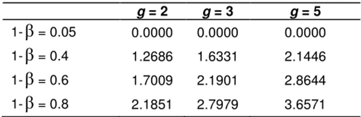
Table 1. Values of

Γ

_k according to the 4 values of 1- .

g = 2 g = 3 g = 5

1- = 0.05 0.0000 0.0000 0.0000 1- = 0.4 1.2686 1.6331 2.1446 1- = 0.6 1.7009 2.1901 2.8644 1- = 0.8 2.1851 2.7979 3.6571

18; three values of the common size sample,

n

were considered for each value of

p

:

n/

p

= 1.5;

n/

p

=2.5 and

p

n/

=5. For each number g of groups, four values of the heteroscedasticity degree,

Γ

_k (

k

=

2, 3 and 5) of the populations were chosen from established empirical power function, 1- of the homoscedasticity test related to

Γ

_k under normality case (1- =0.05: homosceda-sticity; 1- =0.4: low heteroscedasticity; 1- =0.6: average heteroscedasticity; 1- =0.8: high hetero-scedasticity. Table 1 presents for each number of groups, the mean values of

Γ

_k related to each of the four values of 1- . Three values of the overlap,

e

of the populations were considered:

e

=0.05 (low overlap);

e

=0.1 (average overlap) and

e

=0.15 (high overlap). The group-prior probabilities were considered equal and the overlap was then equal to the optimal error rate. For each of the combination of population features described above, the values of the parameter m (defined in section 4.1) were iteratively computed to obtain each of the three values of the overlap (or optimal error rate) of the populations. However, the expression (2.3) for the computation of the overlap, e was difficult to manipulate for g>2 so that we used an empirical approach to compute the overlap,

e

.

We presented below (without loss of generality), the computational method of

e

for three p-variate populations,

P

₁ ,

P

₂ and

P

₃ , of theoretical density func-tions

f

₁ ,

f

₂ and

f

₃ . In the discriminant model consi-dered in section 4.1, the differences between the means vectors were only carried by the first two variables of the populations. In such cases, the other variables did not influence the overlap,

e

of the populations. So, it can be deduced from (2.3) that, for equal group-prior probabilities:

e

=

(

)

3

222 Afr. J. Math. Comput. Sci. Res. ∈ > > ∈ > > + = 1 2 3 1 3 1 3 2 1 2 ( ) ( )and ( ) () P 1 P ) ( ) ( and ) ( ) ( 1 1 ( ) ( ) x x x x f x f x x f x f x f x f dxdy x f dxdy x f e f f ; ∈ > > ∈ > > + = 2 2 3 1 3 2 3 1 2 1 ( ) ( )and () ( ) P 2 P ) ( ) ( and ) ( ) ( 2 2 ( ) ( ) x x f x f f f x x f x f f f dxdy x f dxdy x f e x x x x ; (4.3) ∈ > > ∈ > > + = 3 3 2 1 2 3 3 1 2 1 ( ) ( ) and ( ) ( ) P 3 P ) ( ) ( and ) ( ) ( 3 3 ( ) ( ) x x f x f x f x f x x f x f f f dxdy x f dxdy x f e x x

In (4.3),

e

₁,

e

₂ and

e

₃ represented the group-conditional error rates of the Bayes rule. The used empirical approach considered these conditional error rates as the volume of solids constituted of successive elementary volumes of width,

dx

(

dx

=

x

_i+1

−

x

_i ), length,

dy

(

dy

=

y

_i+1

−

y

_i ) and height, the value of the bivariate probability density function at

dx

(dx,dy

)

. The same method was used in the case of 2 and 5 groups.

A total of 1728 combinations of the factors were considered and for each of them, 100 samples of size

gn

were generated from the g populations. For each of them, the 10 non parametric error rate estimators were computed. The actual error rate

ec

was also empirically computed for each sample by validating the established linear rule on a large sample of size 10,000g and used to calculate the Relative Error (

RE

), the Relative Bias (

RB

) and the Relative Efficiency (

RE

ff ) of each estimator:

RE

=

ec

ec

−

estimator

100

;

RB

=

ec

ec)

(estimator

100

−

; ff

RE

=

min(RE)

or)

RE(estimat

_{. (4.4)}

In (4.4), the symbol min(RE) represented the relative error of the best estimator for the considered sample. The Mean Relative Error (MRE), the Mean Relative Bias (MRB) and the Mean Relative Efficiency (MREff) related

to each estimator were computed for each of the 1728 combinations of the factors.

RESULTS

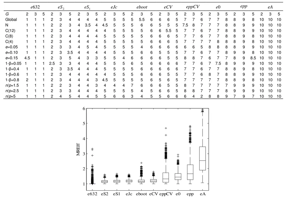
The MRE of the non-parametric estimators for each combination of the factors were replaced by ranks. For a given combination of the factors, the ranks of the error rate estimators were computed, the estimator of the lowest relative error having the rank 1. The median ranks of the estimators were calculated for each factor level as

well as their median rank for all the 1728 combinations of factors and placed in Table 2.

It can be noticed that

e

632

is the overall best estimator; the other estimator of good performance were

2

eS

and

eS

₁ . On the contrary,

e

0

,

epp

and

eA

recorded the lowest relative efficiencies. The ranks of the ten estimators for each level of population features did not globally depend on the number g of groups, except

2

eS

estimator whose relative performance slightly decreased with increased number of groups. The population features seemed not to have influenced the ranks of the estimators. However,

eboot

and

eppCV

improved their ranks for increased values of the ratio

n/

p

whereas opposite trend was observed in the case of

eJc

but also

eS

₁ and

eS

₂, especially for 5 groups. Moreover, the relative efficiency of

eppCV

and

e

632

became low with the increased overlap of the populations. The median rank of the estimators for the levels of population features did not help to analyse the quantitative difference between their performances. Boxplots of the mean relative efficiencies (MREff) of the error rate

estimators were presented in Figure 1.

This figure confirms the best performance of

e

632

, but also of

eS

₂,

eS

₁,

eJc

,

eboot

and

eCV

with how-ever, a loss of efficiency of about 28% of the latter compared to

632

e

, which is equivalent to a mean relative error of 12.8% for these estimators for 10% of relative error for

632

e

. Except the resubstitution estimator,

eA

that presented a loss of efficiency of more than 100% compared to e632, the other estimators presented losses of efficiency that vary from 28% to 70% compared to e632. As far as the dispersion of the MREff of the estimators was concerned, Figure 1 shows the very low variability of

e

632

, which maintained its best performance over the various populations features considered in the study. Estimators

eppCV

,

e

0

,

epp

and

eA

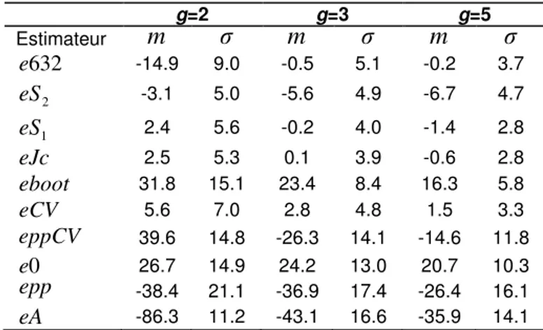
that presented the lowest performance were also the less stable.

The Mean Relative Bias (MRB) helped to appreciate the direction of the deviation of the estimators’ performance for 2, 3 and 5 groups. Table 3 shows that almost all the non parametric estimators performed well when the number of groups became more important. For 2 and 3-group discriminant analyses,

eS

₁ and

eJc

pre-sented the lowest absolute MRB (2.5% for 2 groups and 0.1 for 3 groups) whereas for 5 groups,

e

632

became the best with 0.2% of absolute MRB. The resubstitution estimator,

eA

presented the most optimistic bias whereas

e

0

presented the most pessimistic one.

Kakaï et al. 223

Table 2. Median ranks of the estimators according to the populations features.

632

e

eS

2

eS

1

eJc

eboot

eCV

eppCV

e0

epp

eA

G 2 3 5 2 3 5 2 3 5 2 3 5 2 3 5 2 3 5 2 3 5 2 3 5 2 3 5 2 3 5 Global 1 1 1 2 3 4 4 4 4 5 5 5 5 5.5 6 6 6 5 7 7 6 7 7 8 8 9 8 10 10 10 N 1 1 1 2 2 3 4 3.5 4 4.5 5 5 5 6 6 5 5 5 7.5 8 7 7 7 8 8 9 9 10 10 10 C(12) 1 1 1 2 3 4 4 4 4 4 5 5 5 5 6 6 5.5 5 7 7 6 7 7 8 8 9 9 10 10 10 C(8) 1 1 1 2 3 4 4 4 4 5 5 5 5 5 6 6 6 5 7 7 6 7 7 8 8 9 8 10 10 10 C(4) 1 1 1 2 3 4 4 4 4 5 5 5 5 5 6 6 6 5 7 7 7 7 8 8 8 9 8 10 10 10 e=0.05 1 1 1 2 3 3 4 5 4 5 5 5 5 4 6 6 6 6 6 6 5 8 8 8 8 9 9 10 10 10 e=0.10 1 1 1 2 3 3.5 4 4 4 4 5 5 5 6 6 5 5 5 7 7 6 7 7 8 9 9 8 10 10 10 e=0.15 4.5 1 1 2 3 5 4 3 3 5 5 4 6 6 6 6 5 5 8 8 7 6 7 7 8 9 8.5 10 10 10 1- =0.05 1 1 1 2.5 3 3 4 4 4 5 5 5 6 5 6 6 6 6 7 7 6 7 7.5 8 9 9 9 10 10 10 1- =0.4 1 1 1 2 3 3.5 4 4 4 5 5 5 5 6 6 6 6 6 7 7 6 7 7 8 8 9 8 10 10 10 1- =0.6 1 1 1 2 3 4 4 4 4 4 5 5 5 6 6 6 5 5 7 7 6 8 7 8 8 9 9 10 10 10 1- =0.8 2 1 1 2 3 4 4 4 3 4.5 5 5 5 5 6 5 6 5 7 7 7 7 7 8 8 9 8 10 10 10 n/p=1.5 1 1 1 2 2 3 4 4 3 4 4 4 7 6 6 6 5 5 8 7 7 7 7 7 9 9 9 10 10 10 n/p=2.5 1 1 1 2 3 3 4 4 4 5 5 5 5 4 5 6 6 5 8 8 7 7 7 8 9 9 9 10 10 10 n/p=5 1 1 1 2 4 5 4 4 5 5 6 6 3 4 5 5 6 6 6 4 2 8 8 9 7 9 7 10 10 10

e632 eS2 eS1 eJc eboot eCV eppCV e0 epp eA 1 2 3 4 5 6 M R Ef f

224 Afr. J. Math. Comput. Sci. Res.

Table 3. Mean and standard deviation of the MRB of the error rate

estimators. g=2 g=3 g=5 Estimateur

m

m

m

632 e -14.9 9.0 -0.5 5.1 -0.2 3.7 2

eS

-3.1 5.0 -5.6 4.9 -6.7 4.7 1

eS

2.4 5.6 -0.2 4.0 -1.4 2.8

eJc

2.5 5.3 0.1 3.9 -0.6 2.8

eboot

31.8 15.1 23.4 8.4 16.3 5.8

eCV

5.6 7.0 2.8 4.8 1.5 3.3

eppCV

39.6 14.8 -26.3 14.1 -14.6 11.8 0 e 26.7 14.9 24.2 13.0 20.7 10.3

epp

_{-38.4 21.1 -36.9 17.4 -26.4 16.1}

eA

-86.3 11.2 -43.1 16.6 -35.9 14.1

DISCUSSION AND CONCLUSION

The estimation of the actual error rate for practical use is one of the relevant topics in discriminant studies and a synthesis of the various estimators of the actual error rate was provided in McLachlan (1992). Most studies have been done to compare in two group-discriminant analysis the performance of the error rate estimators, especially associated with the linear classification rule and a synthesis of them was done by Schiavo and Hand (2000). The originality of our study is that the relative efficiency of non parametric error rate estimators can be analysed in multi-group discriminant analysis. The obtained results helped to point out the overall best efficiency of e632 irrespective of the number of the considered groups. For two-group linear discriminant analysis many studies came almost to the same conclusions (Glèlè Kakaï and Palm, 2009; Wehberg and Schumacher, 2004; Glèlè Kakaï et al., 2003). Other studies pointed out the efficiency of this estimator for non linear classification rules. Jain et al. (1987), using multivariate normal distributions in nearest neighbour discriminant analysis, found that e632 outperformed all the other estimators (

eCV

,

eboot

,

e

0

). However, we noticed from the present study that for high overlap of the populations in the case of two groups, the performance of this estimator decreased. Fitzmaurice et al. (1991), using two-group discriminant analysis concluded that e632 became less reliable as the true actual error rate increased above 0.35, but more reliable as the true error rate decreased. Other estimators that performed well in the present study were

eS

₁ ,

eS

₂ and

eJc

. On contrary,

0

e

,

epp

,

eppCV

and

eA

recorded the lowest perfor-mance, in most of the cases considered in the study.

The ranks of estimators were less influenced by the populations’ features, probably due to the fact that they were all based on resampling methods that do not neces-

sitate conditions of use. However, the number of groups had a high impact on the performance of the estimators. The later became more efficient as the number of group increased.

The highest positive relative bias was obtained by

eA

whereas

e

0

has the highest and negative relative bias. These results have been already obtained by Wehberg and Schumacher (2004), Chatterjee and Chatterjee (1983) and Chernick and Murthy (1985) who qualified eA and

e

0

as the optimist and pessimist estimators, respectively.

ACKNOWLEDGEMENTS

This work was supported by the Alexander-Von-Humboldt Foundation (AvH) and the Third World Academy of Sciences (TWAS).

REFERENCES

Chatterjee S, Chatterjee S (1983). Estimation of misclassification probabilities by bootstrap methods. Communication in Statistics – Simulation and Computation. 12: 645-656.

Chernick MR, Murthy VK (1985). Properties of bootstrap samples. Am. J. Math. Manage. Sci.5:161-170.

Efron B (1983). Estimating the error of a prediction rule: improvement on cross-validation. J. Am. Stat. Assoc. 78: 316-331.

Fitzmaurice GM, Krzanowski WJ, Hand DJ (1991). A Monte Carlo study of the 632 bootstrap estimator of error rate. J. Class. 8: 239-250. Fukunaga K, Kessell DL (1972). Application of optimum error reject

function. IEEE Trans. Infor. Theor.18: 814-817.

Glèlè Kakaï R., Palm. R. (2006). Methodological contribution to control heteroscedasticity in discriminant analysis studies. Glob. J. Pure. Appl. Sci. 12 (1) : 107-110.

Glèlè Kakaï R, Palm R (2009). Empirical comparison of error rate estimators in logistic discriminant analysis. J. Stat. Comput. Simul. 79(2): 111-120.

Glèlè Kakaï R, Piraux F, Fonton N, Palm R (2003). Comparaison empirique des estimateurs de taux d’erreur en analyse discriminante. Revue de Statistique Appliquée. 51(2): 91-104. Hand DJ (1986). Recent advances in error rate estimations. Pattern

Recog. Lett. 4: 335-346.

Jain AK, Dubes RC, Chen C (1987). Bootstrap techniques for error rate estimation. IEEE Transactions on Pattern Analysis and Machine Intelligence. 9: 628-633.

Lachenbruch PA (1967). An almost unbiased method of obtaining confidence intervals for the probability of misclassification in discriminant analysis. Biometrics. 23: 639-645.

McLachlan GJ (1975). Confidence intervals for the conditional probability of misallocation in discriminant analysis. Biometrics. 31: 161-167.

McLachlan GJ (1992). Discriminant analysis and statistical pattern recognition. Wiley,New York.

Quenouille MH (1949). Approximate tests of correlation in time series. J. R. Stat. Soc. (Serie B).11: 18-84.

Schiavo RA, Hand DJ (2000). Ten more years of error rate research. Int. Stat. Rev. 68: 295-310.

Smith CAB (1947). Some examples of discrimination. Ann Eugen. 13: 272-282.

Wehberg S, Schumacher M (2004). A comparison of Nonparametric Error Rate Estimation Methods in Classification Problems. Biom. J. 46: 35-47.