Public pension wealth and household asset holdings: new evidence from Belgium

(1)

1

Public pension wealth and household asset holdings: New evidence from Belgium

Mathieu Lefebvre BETA, University of Strasbourg

Sergio Perelman

HEC-University of Liège and CREPP

Abstract

It has been long suggested that public pension wealth may crowd out household savings. However, there remains controversy about the extent of this displacement effect. In this paper we use an original microsimulation model based on retrospective survey data collected through the third wave of the Survey of Health, Ageing and Retirement in Europe (SHARE) to estimate the displacement effect of public pension wealth on other wealth in Belgium. Combining this rich dataset with an accurate estimation of the individual pension entitlements allows us to circumvent some of the main measurement errors problems faced by previous studies. We estimate that an extra euro of public pension wealth is associated with about 14-25 cent decline in households’ non-pension wealth.

JEL codes: D91, H55, E21, J14.

Keywords: public pension wealth, saving, microsimulation, displacement effect.

Corresponding author: Mathieu Lefebvre, 61 avenue de la forêt Noire, 67085 Strasbourg, France Tel: 0033 3 68 85 21 71, Email: Mathieu.lefebvre@unistra.fr

Acknowledgments: The authors would like to thank the editor and one anonymous referee for very helpful comments. They would like to thank also participants of seminars at GATE-CNRS, Antwerp University and the Belgian SHARE users’ workshop 2017. The financial support from the Belgian Science Policy Office (BELSPO) research project CRESUS is gratefully acknowledged. This paper uses data from SHARE Waves 2 and 3 (SHARELIFE) (10.6103/SHARE.w2.260, 10.6103/SHARE.w3.100, 10.6103), see Börsch-Supan et al. (2013) for methodological details. The SHARE data collection has been primarily funded by the European Commission through FP5 (QLK6-CT-2001-00360), FP6 (SHARE-I3: RII-CT-2006-062193, COMPARE: CIT5-CT-2005-028857, SHARELIFE: CIT4-CT-2006-028812) and FP7 (SHARE-PREP: N°211909, SHARE-LEAP: N°227822, SHARE M4: N°261982). Additional funding from the German Ministry of Education and Research, the U.S. National Institute on Aging (U01_AG09740-13S2, P01_AG005842, P01_AG08291, P30_AG12815, R21_AG025169, Y1-AG-4553-01, IAG_BSR06-11, OGHA_04-064) and from various national funding sources is gratefully acknowledged (see www.share-project.org).

(2)

2

Public pension wealth and household asset holdings: New evidence from Belgium

1. Introduction

Given the important demographic challenges that most developed countries are facing, it has been long suggested that they should reform their social security systems. Especially it is often argued that public pension generosity should be reduced in order to cut budgetary spending but also to induce higher labor force participation at older ages. While such reforms may have an impact at different level, it has also been suggested that pension benefits may actually crowd out household savings such that changes in public pension legislation and generosity could have important welfare effects (Alessie et al, 2013).

If there exists important substitutability between pension wealth and household savings, downsizing reforms of social security generosity should induce households to save more. If a decrease in pension benefits is not followed by an increase in household savings then the available resources at retirement will be reduced. Understanding the effect of public pension reforms on private saving is then of great importance, especially when, as in most developed countries, reforms of the pension systems are being considered.

In this paper we present new estimates of the displacement effect of public pensions on household wealth using data for Belgium collected by SHARE. Following Alessie et al (2013), we rely on the retrospective nature of the data from the third wave of the survey (SHARELIFE) which contains information on the entire career of older workers and retirees. These data are used to construct a measure of the present value of past earnings using the entire job history of each respondent and the information on the first wage earned in each job. The novelty of our approach come from the use of an original microsimulation model (Jousten and Lefebvre, 2013; Jousten et al, 2016) to accurately compute expected pension wealth for those who are not

(3)

3

retired. Most of previous studies instead had to rely on proxy measures and Alessie et al (2013) used subjective information on individuals expected replacement rate to compute expected pension wealth.

We believe that the microsimulation allows us to tackle some of the measurement issues. Especially the measurement errors in measures of lifetime earnings and pension wealth when they are not observed. Alessie et al (2013) point the fact that these two measurement errors can be positively correlated with each other; which can lead to a spurious partial correlation between pension wealth and household savings. By using a microsimulation, the calculation of the pension benefit takes into account the actual rules of the social security administration but also relies on the non-linearity of the pension formula. This is particularly important in Belgium where there are floors and ceilings applied both to lifetime incomes and pension amounts. And there are also specific rules for the computation of pension benefits for individuals who, during their working career, were subject to different public pension schemes. In addition, the microsimulation allows us to calculate the pension entitlements for any individual. This means we can then estimate the displacement effect both for men and women (for whom data are often scarce) as well as at the household level.

Several authors have tried to estimate empirically the relationship between pension wealth and private wealth and their results are not conclusive. In his seminal paper, Feldstein (1974) using time-series aggregate saving rates indicated a displacement effect of pension wealth on household savings of about -40 cents per dollar of pension benefits. Since then many papers have used microeconomic data sets (mainly cross-sectional household studies) to investigate the level of the displacement effect, in the US and in Europe. The results go from an offset close to zero to an offset close to 100% of non-pension wealth with respect to each unit of pension

(4)

4

wealth1_.

The wide range of estimates is due to the variety of empirical methodologies across studies. It reflects also the difficulty to correctly identify and estimate the relationship between the provision of pension benefits and household savings. Indeed the presence of unobserved heterogeneity makes it difficult to identify the effect of different levels of pension wealth on different saving behavior. Particularly Gale (1998) shows that regressing non-pension wealth on pension wealth and other cash earning variables provide biased downward crowd-out estimates. He stresses the importance to adjusting pension wealth for the age of the individual. Because of unobserved differences in saving behavior, there is likely positive correlation between wealth and retirement age. He suggests removing the bias by applying an adjustment factor to pension wealth that takes into account the age of the individual, the so-called Gale’s Q.

As pointed above another important issue concerns the difficulty to obtain an accurate measure of lifetime earnings and pension wealth as well as an accurate measure of private wealth. The problem is that most household surveys do not provide measures of lifetime earnings so that most of studies rely on proxy measures for lifetime earnings which makes difficult to obtain an accurate measure of pension wealth. Recently, Engelhart and Kumar (2011), using data on older workers from the US Health and Retirement Study, adopt an instrumental variable approach to account for the measurement error in pension wealth and circumvent these difficulties. Hurd et al (2012) aggregate cross-country data by education and marital status to tackle problems with

1_{Among others, see Feldstein and Pellechio (1979), Kotlikof (1979), Hubbard (1986), Gale (1998) for the US;}

Dicks-Mireaux and King (1984) for Canada; Attanasio and Rowhedder (2003) for the UK; Jappelli (1995), Attanasio and Brugiavini (2003) for Italy; Alessie et al (1997) for the Netherlands; Klump and Kim (2010) for Germany; Blanchet et al (2016) for France; Lachowska and Myck (2015) for Poland; Hurd et al (2012), Alessie et al (2013) for cross-country analysis.

(5)

5

omitted variables and measurement errors. The problem is that even when they are observed, both present value of past and future earnings and pension wealth are measured with errors which can bias the estimates of the displacement effect.

Using retrospective data from the Survey on Health, Ageing and Retirement in Europe (SHARE), Alessie et al (2013) propose a restricted model for which they can sign the impact of correlated measurement errors on the estimators. They provide “lower bound” estimates using a sample of retirees for whom they know lifetime income and pension wealth come from two independent series of surveys questions. While these two variables are possibly measured with errors, the correlation between these measurement errors is likely to be small.

As indicated before, our estimation for Belgium is also based on SHARE retrospective data, but relies on a detailed microsimulation model to compute pension wealth. We find evidence of a modest displacement effect of 14% to 25 % of public pensions on private wealth depending on the econometric specification. The estimated effect is significantly different from zero and -1. These results are different than those found by Alessie et al (2013) with their full sample of SHARE countries. However our results are much in line with the lower bounds they obtained for a subsample of retirees for whom the effect of measurement errors is likely to be small.

In a robustness section we show that the difference seems to be directly related to the estimation of the pension wealth that in our case is obtained taken into account all the social security rules and for which we can expect the correlation between the measurement errors to be reduced. It is worth to add that our results depend on the availability of a detailed microsimulation model of pension rights which is difficult to be undertaken for several countries. A notable exception has been the International Social Security project of the NBER which has shown the usefulness of such a method in a comparative framework (see i.e. Gruber and Wise, 2004 and 2007).

The rest of the paper is organized as follows. Section 2 outlines the institutional background of the Belgian pension schemes. Section 3 presents a simple life-cycle framework that will guide

(6)

6

the empirical specification. We then present in Section 4 our data as well as the variables and the microsimulation we use. Section 5 presents the results, including robustness checks, and Section 6 concludes.

2. Institutional framework

The Belgian public retirement system is characterized by three large sectoral schemes, one for the private sector wage-earners, one for the public sector and one for the self-employed2_{. The}

main system is the wage-earners public pension scheme. Individuals are eligible to full benefits at the age of 65 but it allows voluntary retirement from age 60. The pension benefit corresponds to 75% of average lifetime earnings for one-earner couples and to 60% for others. There are floors and ceilings for earnings taken into account, fully updated for inflation but only partially for real wages growth. A full career corresponds to 45 years of earnings or assimilated periods. Indeed a peculiar feature of the system is that period of one’s life spent on replacement income (such as unemployment or disability) fully counts as years worked in the computation of the retirement benefits. For any such periods, wages from previous periods at work are inserted into individuals’ records file. Benefits are shielded against inflation through an automatic price adjustment and are subject to an earning test.3

The system for self-employed is very similar to the wage-earners. Full public pension benefits are available at age 65 with a complete earnings history of 45 years, as in the private sector scheme. Benefits are based on average earnings but for the years before 1984, a lump-sum amount is taken into account. However, in practice, wage-earners pension benefits are in

2_{A good review of the various Belgian public pension schemes can be found in Dellis et al (2004) and Jousten et}

al (2012). The main features of these schemes kept unchanged over several decades. The only exception was the increase of women normal age of retirement in 1997, from 60 to 65 to reach that of men, with a transition period going to 2009.

3_{Minimum pension benefits and pensions paid to oldest pensioners are also updated regularly to take into account}

(7)

7

average near 50% higher that self-employed benefits.4 The main reason explaining this gap is

that professional earnings entering in the computation of self-employed pensions are only partially considered. More precisely, earnings are multiplied by a fraction which corresponds to the ratio between self-employed and wage-earners payroll taxes rates (0.541 and 0.663 for earnings above or below the 31,820€ threshold in 2016, respectively (INASTI-RSVZ, 2017)).

Civil servants face compulsory retirement at the latest at age 65 but it is possible to opt for early retirement. Public sector pensions are based on the income earned during the last five years before retirement. Benefits are equal to 75%, at maximum, of the average wages over the last five years. The system also applies floors and ceilings which are much more generous than in the private sector. Public pensions are indexed on average wages in the public sector, which make them much more advantageous for higher-income individuals. In average, 28.296€ is the average annual amount of before tax civil-servant pensions in 2015. That is more than double of wage-earner pensions (PDOS-SDPSP, 2016).

Overall it is possible to accumulate rights in several schemes and to obtain a kind of a mixed pension. This case is frequent and then each scheme accounts for a part of the total pension benefits. Nevertheless, Belgian public pension benefits reflect generosity differences across schemes and are highly dispersed. As a direct consequence, public pension wealth is also unequally distributed across individuals and households, and in this paper we try to estimate how, and to which degree, pension rights are substitute for wealth accumulation.

3. Theoretical framework and empirical specification

We follow Engelhardt and Kumar (2011) and Alessie et al (2013) who consider a simple life-cycle model formulated by Gale (1998). Especially we follow Alessie et al (2013) who derive

4_{Average annual pension benefits for pensioners with wage-earner and self-employed exclusive careers were}

14,549€ and 9,990€, respectively (own computations based on pension beneficiaries statistics from ONP-RVP (2016).

(8)

8

the equation of interest from a simple discrete-time counterpart of the model. We assume that an individual lives from period 1 to period T and retirement occurs at time R. Utility is derived from consumption and is assumed to be isoelastic and exhibits constant relative risk aversion (CRRA). The consumer maximizes lifetime utility:

max (1 + 𝜌) 𝐶

1 − 𝛾 (1)

subject to the intertemporal budget constraint

(1 + 𝑟) 𝐶 = (1 + 𝑟) 𝑌 = (1 + 𝑟) 𝐸 + (1 + 𝑟) 𝐵 (2)

where 𝐶 and 𝑌 denote respectively consumption and income at time 𝜏 wherein 𝐸 is labor-market earnings and 𝐵 is public pension benefits; r is the constant real interest rate, 𝜌 is the

discount rate and 𝛾 is the coefficient of relative risk aversion.

Maximization of (1) subject to (2) implies:

𝐶 = 𝐶 1 + 𝑟 1 + 𝜌 (3) 𝐶 =∑ (1 + 𝑟) (𝐸 + 𝐵 ) ∑ 𝜆 (4) where 𝜆 = (1 + 𝑟) 1 + 𝑟 1 + 𝜌

(9)

9

Because we are interested in the impact of public pension wealth on wealth accumulation, we can express non pension wealth at a given age t, 𝐴 , as the cumulative difference between income and consumption and substituting (3) and (4), we obtain:

𝐴 = (1 + 𝑟) (𝑌 − 𝐶 ) = (1 + 𝑟) 𝑌 − 𝑄 (1 + 𝑟) 𝑌 (5)

Where 𝑄 =_∑∑ is the Gale’s Q, which when 𝜆 ≠ 0, takes into account the time the

consumer has had since the introduction of the pension to adjust the lifetime consumption stream (Gale, 1998). Finally, using equation (2), equation (5) can be rewritten

𝐴 = (1 + 𝑟) 𝑦 − 𝑄 (1 + 𝑟) 𝐸 − 𝑄 (1 + 𝑟) 𝐵 ₍₆₎

where 𝑃 which denotes the Gales-Q-adjusted pension wealth and 𝐼 is the adjusted lifetime income. Based on equation (6), our empirical strategy is to estimate the following regression:

𝐴 = 𝛽 + 𝛽 𝐼 + 𝛽 𝑃 + 𝑋 𝛾 + 𝜀 (7)

where 𝑋 is a vector of individual characteristics that may affect savings. Indeed there are factors that are not taken into account in the theoretical model that may affect the relationship between wealth and the flow of earning and pensions. In equation (7), the primary variable of interest is 𝑃 and 𝛽 measures the impact of an additional euro of pension wealth on non-pension wealth.

4. Data

The empirical analysis uses data from the Survey of Health, Ageing and Retirement in Europe (SHARE). The survey is a cross-national panel database of micro data on health, socio-economic status and social and family networks of European individuals aged 50 and over conducted since 2004-05. It covers a broad range of variables of special interest for this study

(10)

10

such as information on employment, income, real and financial assets and the household context. The first wave of collection was in 2004/05 and there are now five waves available. Our sample of analysis is based on individuals aged between 55 and 85 in wave 2 (2006/07) in Belgium5_.

The third wave of data from SHARE, known as SHARELIFE (collected in 2008-09), asked all previous respondents (waves 1 and 2) and their partners to provide information not on their current situation but on their entire life–histories. This provides retrospective information on childhood, health, living and professional career. Thanks to the data from SHARELIFE we are able to reconstruct the individual’s career history. SHARELIFE asks the respondents to provide start and end dates of each paid job they had, the characteristics of the job, as well as the first monthly wage. For those who are still employed at the time of the interview, the last monthly wage is asked and for those who are already retired the last monthly wage in the main job is asked. All these amounts are after taxes, as are the amount in the wave 2 of SHARE.

This information is used to construct a panel with one observation per year for each individual, from the first job until the interview year. These data are used to calculate the various income flows entering 𝐼 . The wage path is obtained using linear interpolation between the years for which we have wage information; that is between the different wages declared along the career and the last wage of the main job or the current wage of the employed. For years spent under replacement income (i.e. unemployment, disability, sickness …), we use actual rules applied in Belgium to calculate the benefit given occupation, earnings and family status6_{. Once computed}

in this way the complete career path, the amounts are converted in Euros of the interview year.

5_{There are two reasons for using only the second wave of the survey. First we need to concentrate on waves that}

are earlier to the third wave, SHARELIFE. Second in the first wave the wages and pensions were elicited before taxes but after taxes in the second wave.

6_{Fortunately, rules of calculation of unemployment and disability benefits have not changed much during the last}

(11)

11

In the paper we use a constant annual interest rate (r) of 0.03, as in Alessie et al (2013) and compounded labor income is obtained starting from the year of the first job for the retirees. Future labor income is calculated for the employed assuming constant real wages. Retirement is assumed to start in the year that the individuals declare as their expected retirement age or the statutory retirement age (65 in Belgium) if they did not specify their expectations. All future incomes are weighted by the individual probability of survival using life tables from the Human Mortality Database (2015)7_.

Public pension benefits are obtained through two channels. For those who are already retired, the level of benefits is the one declared in the survey. For those still employed, we use a microsimulation developed for Belgium on the basis of SHARE data (see Jousten and Lefebvre, 2013; Jousten et al, 2016). This allows us to calculate precise value of the entitlement of each individual in the survey given the actual rules applied in Belgium. Pension wealth, 𝑃 , is calculated applying survival probabilities from the Human Mortality Database and assuming constant real benefits as well as discount rate (ρ) of 0.03. The Gales-adjustment factor, Q, is obtained with 𝜆 = 0.03.

The non-pension wealth, 𝐴 , is available in wave 2 at the household level. We use household net worth and its decomposition into net real wealth and net financial wealth. In SHARE data, missing values for individual and household level economic information are replaced by five imputed values for each missing ones (see Christelis, 2011). This is the case of wealth variables so that in all estimations below we use multiple imputations techniques (see Rubin, 1987). The net real wealth is the sum of the value of the main residence minus any mortgage, the value of other real estate, the value of own share of businesses and the value of own cars. The net financial wealth is the sum of gross financial assets minus (non-mortgage) debts.

(12)

12

Finally we include a set of explanatory variables, 𝑋 , to capture individual differences. In the following regressions we use age, gender, marital status, education level, self-declared health, number of children and spouse.

Our sample of analysis is based on individuals in wave 2 (2006/07) of SHARE in Belgium and for whom we have information in SHARELIFE. This amounts to 2,340 observations. We concentrate on individuals aged between 55 and 85 (1531 observations) and we exclude those who have never worked or for whom we do not have enough career information in order to construct the wage path (449 observations). We keep those who had a short career since the Belgium system does not penalize short career and applies fictitious wages to period under replacement income (see Section 2). We end up with a sample of 1,082 observations.

Our sample is rather large compared to previous studies using SHARE in a cross-country analysis because the microsimulation allows our sample not being too much affected by missing values and erroneous answers. Furthermore, it is even more valuable at the time of calculating the pension entitlement. Alessie et al (2013) calculated the pension entitlement of those still working by multiplying the expected replacement rate by the current salary. The microsimulation developed for Belgium allows us to obtain much more accurate measures. As an example, when we compare the average annual pension benefit according to the two methods, we obtain diverging results both in terms of average and standard deviation. Individuals would systematically overestimate their forthcoming pension8.

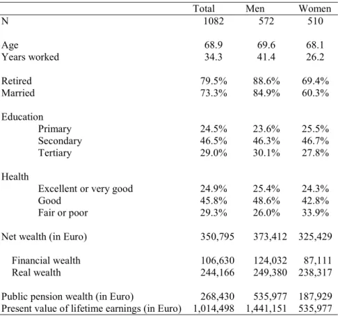
Table 1 presents descriptive statistics for the sample. It is well balanced between men and women and the average age is about 69 years old. The length of working career is about 34 years and women have shorter career than men. Almost 80% of the sample is retired and

8_{In our sample, the pension benefit obtained though the use of the expected replacement rate is on average €14.325}

(13)

13

surprisingly this number rises to 88.6% for men while it is only 69.4% for women. Looking at the proportion that is married, we observe that only 60.3% of women are married while 84.9% of men are. Thus women in our sample are more active than men and this likely comes from our sample making constraint in which we have excluded individuals who have never worked. In the female population, it is a kind of all or nothing career decision. Those who were married and never worked, particularly women, are thus not represented in our sample. This also explains why in our sample we have more single active women than single men. Table 1 also presents the total net wealth and shows that the main part of the wealth is non-financial, especially for women. In table 1 we also find the non-adjusted value of pension wealth (that is before Gale Q-adjustment) and lifetime income.

Insert Table 1

5. Results

Table 2 presents the estimation of 𝛽 and 𝛽 (following the model represented in equation (7)) for the Ordinary Least Squares (OLS) estimators but also using robust regression and median regression techniques to limit the impact of outliers, as in Gale (1998) and in Alessie et al (2013). As explained in Section 4, due to multiple imputations for missing variables of our dependent variables, the estimations are based on the imputed data and coefficients and standard errors are adjusted for the variability between imputations, see Rubin (1987) and Little and Rubin (2002)9_{. Each regression includes age, age squared, marital status, gender, the number}

of children, education and health as controls 10_.

9_{SHARE presents five different imputations for the net wealth. Practically, regression estimations are executed on}

each of the five imputed variables to obtain five sets of coefficients and standard errors. These five estimates are then combined to obtain a set of inferential statistics. We have also estimated the same regressions without multiple imputations but clustering standard errors for repeated information within the household and it does not change much our results. Significance is identical. Results are available upon requests.

(14)

14

The results indicate a displacement effect between 14% and 24% and this effect is significantly different from 0 and 100% whatever the regression. Robust and median regressions display similar results although much lower than OLS estimates. This means that an additional euro of pension wealth decreases the net wealth by 14 to 24 cents. Interestingly, the lifetime income,

𝐼 , displays a positive and significant effect on savings. In all specifications, except OLS11_{, the}

coefficient of lifetime income is bigger in absolute value than pension wealth. Thus the effect of pension wealth on household’s private savings is lower than the effect of income. Whereas they are not presented here, some of the control variables display significant effects. Being married and highly educated results in higher wealth but having a bad health decreases the amount of accumulated wealth.

Insert Table 2

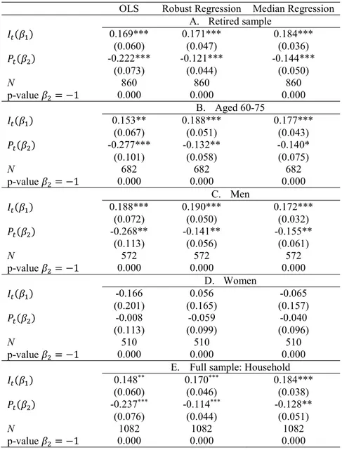
These results are much in line with the lower bounds presented by Alessie et al (2013) using the same source of data but many more countries. However as in order to check the robustness of our results, we estimate the model on a subsample of retirees. For this particular subsample, if there are measurement errors in 𝐼 and 𝑃 , they are likely to be uncorrelated since the two variables are obtained from a different set of questions in SHARE. The panel A in Table 3 presents the estimation for the retirees only. We do not find qualitatively different results than those obtained with the full sample which tend to confirm the accurateness of results presented in Table 2.

Our sample consists mainly of retirees (860 over 1,082 observations) which is not surprising given the very low labor force participation of older workers in Belgium. Since the retirement decision might be endogenous, it could lead to endogenous sample selection. Thus we also estimate the displacement effect on a subsample that is based on the age of the individuals rather

11_{The difference shows the importance of controlling for outliers and measurement errors in the dependent}

(15)

15

than on their retirement status. Panel B in Table 3 displays the results when we restrict our sample to those aged between 60 and 75. That is that we do not select the sample based on retirement status but simply using an age criterion that is close to the average age of retirement in Belgium. Again the results are similar which makes us confident that our microsimulation allows us to avoid part of the measurement errors in the calculation of pension wealth and above all the correlation between the measurement errors in 𝐼 and 𝑃 .

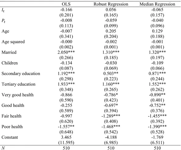
In Table 3, we also estimate the model separately for men and women since they may have very different career history12_{. We have seen in Table 1 than the women have a shorter career, a}

lower lifetime earnings and then a smaller pension wealth than men. Indeed Panel C and D in Table 3 show different displacement effects for men and women. Depending on the model, the effect is between 1.5 and 3 times higher for men than it is for women. Interestingly no regression gives significant effects of income and pension wealth for women. This would conclude that there is no displacement effect for women.

Insert Table 3

However the dependent variable, the total non-pension wealth, is measured at the household level while the public pension wealth is measured at the individual level. In couples, a secondary earner could also build up pension rights. This may be particularly relevant for women who suffer from lower pension wealth. It seems then interesting to consider the sum of pension wealth at the household level since not considering the pension wealth of the partner might also explain why no evidence of crowding-out effect is found for women. Panel E in Table 3 presents the results when we introduce the household pension wealth as an explaining factors of the household non-pension wealth. We still control for individual characteristics as

12_{Women may had broken careers due to children particularly. However our microsimulation of retirement benefits}

(16)

16

in previous regressions. Interestingly, the results are not much impacted and we find similar displacement effect13_.

6. Robustness tests and sensitivity analysis

One important aspect of our estimation is concerned with the measurement errors. Even if there is no correlated measurement error between I and P, there is still a possibility to have measurement error in P, especially for those who are already retired. This may causes an attenuation bias. As exposed above, Alessie et al (2013) used the same SHARE data for a series of countries. They approximated the pension benefits by the individual expectation and they obtained counterintuitive results when they estimated the same model as ours. They push forward the effect of the correlation of measurement errors between the lifecycle income and the pension wealth to explain their results and they show that under the validity of the lifecycle model, by imposing that 𝛽 = 1, they are able to sign the bias associated with the measurement error problem. Their estimation of the displacement effect is still biased but it has the same sign as the true value. Our results exposed above do not seem to be affected by such a problem since we do not find counterintuitive results, especially regarding the sign of the coefficients associated to our variables of interest. This tends to show that the use of full microsimulation model reduce the effects of the measurement errors.

However for sake of comparison, we also estimated the displacement effect using the same pension wealth obtained through the use of the expected replacement rate. This is done in a complete specification as presented above and in a constrained linear regression model. In addition, we present the same constrained model when we use our pension wealth obtained

13_{We could have also presented regression in which we introduce only household level explaining variables. The}

problem is that we do not have much of these to control for. We have tried several specifications (with the size of the household, the average age of the family members and the global income) and it usually gives similar results with a displacement effect around 18%. The results are available upon request.

(17)

17

through the microsimulation model. The results in Table 4 show that indeed when we use their approach to estimate P, we obtain counterintuitive results with 𝐼 being negative and significant and 𝑃 not significant. Once we constraint 𝛽 to be equal to one, we obtain a significant displacement effect but it is much bigger and close to the one obtained in Alessie et al (2013). When we run the same constraint regression with our definition of pension wealth, we still obtain a high displacement effect. These results show the importance of correctly measuring the flow of income from the work career and the pension system. Itappears that our strategy to rely on full microsimulation model allows to circumvent part of the problems related to the measurement errors.

Insert Table 4

In Table 5, we perform a series of additional robustness tests. First we make the distinction between financial and non-financial wealth. Financial wealth, because of its narrowed nature and because it is more dependent on contemporaneous situation, may be unable to detect crowding-out effects, as pension wealth is accumulated over a long period (Alessie et al, 2013; Gale, 1998). However Hurd et al (2012) argued that since financial wealth is more liquid it can then be easily displaced by pension wealth. Our results are in accordance with Gale (1998) and we find a smaller offset when we use a narrowed definition of wealth.

Insert Table 5

Finally, in Table 6, we test for the addition of other covariates that might be relevant in determining non-pension wealth. Since our results so far are qualitatively identical we run these last regressions for the full sample and present only median regressions. First individuals may have different tastes for saving or, saying differently, have different risk preferences. Risk averse individuals are likely to delay retirement age and save more for retirement than risk lovers. We introduce self-declared individual risk preferences taken from a question in

(18)

18

SHARE14_{. Vieider et al (2015) have shown that self-declared measure of risk preferences are}

good measures of the true risk preferences. We introduce a dummy variable equal to 1 if the individual is risk averse. We also control for the partner situation and add in column 2 a dummy variable equal to 1 if the partner is still working and if his/her level of education is higher than 12 years of education in total. Following Alessie et al (2013) we control for whether the individual has ever received inheritances or gifts worth more than 5,000 Euros as well as for the amount received. In Column (1), (2) and (3), our results show that the displacement effect is still in the same range as in Table 2 and significantly different from 0.

Finally, we go one more step forward in identifying different response of household wealth to pensions benefit according to two specific dimensions: education and marital status. As shown in previous works (see Gale, 1998; Engelhardt and Kumar, 2011; Alessie et al, 2013), the displacement effect can be different according to the level of education. Especially, the question of financial literacy (expected to be highly correlated to the level of education) may be important in explaining the various plans for retirement (Solomon, 1975; Bernheim and Garrett, 1996; Bernheim, 1998; Haurin et al, 1996 and Laibson et al, 1998). There can be substantial variation across individuals in the displacement of pensions to saving, with the bulk of crowd-out occurring in the upper levels of education. In table 6, we split our sample according to education and report the estimate for the low and high level of education15_{. We find that the}

displacement effect is not significantly different from zero for the less educated individuals.

14_{The question is « Which of the statements on the card comes closest to the amount of financial risk that you are}

willing to take when you save or make investments?: 1. Take substantial financial risks expecting to earn substantial returns; 2. Take above average financial risks expecting to earn above average returns; 3. Take average financial risks expecting to earn average returns, or 4. Not willing to take any financial risks”. We only consider as risk averse those individuals who selected answer 4.

(19)

19

This tends to confirm previous results that show that less educated people would be less financially literate and thus less able to correctly plan for retirement.

In Table 6, we also look at the differentiated displacement effect according to the marital status. The last columns show that there is no significant displacement effect for the non-married individuals but a significant one for the married. Section 2 has shown how being married or not may affect the pension benefit calculation. Especially the married people can claim for a higher replacement rate if there is only one-earner in the couple making the much more affected by a potential reduction of their benefits. Furthermore, given the larger size of married household compared to non-married ones, a reduction of pensions may be more harmful and then trigger savings reaction.

Insert Table 6 7. Conclusion

This paper provides new evidence about the displacement effect of public pensions on household wealth. We use an original microsimulation model developed to calculate public pension entitlements in Belgium that is based on SHARE data. Using current (wave 2) and retrospective information on lifetime earnings (SHARELIFE) from the SHARE data, we are able to provide convincing estimates of pension wealth both for working and retired individuals.

Our results suggest a displacement effect of roughly 20% (depending on the retained specification) for every additional euro of public pension wealth. This level confirmed lower bounds obtain by previous works when trying to get rid of measurement errors issues (see Alessie et al, 2013; Hurd et al, 2012; Attanasio and Brugiavini, 2003). It is also much lower than previous results obtained with US data (Feldstein, 1974; Attanasio and Rohwedder, 2003; Gale, 1998). These estimates indicate that pension wealth in Belgium is a small but imperfect substitute for household savings. It contradicts the basic prediction of a life-cycle model. We

(20)

20

also show that the displacement effect is much lower (and not significant) for women which was expected given their low labor force participation. Also, we find a similar effect if we take households’ variables instead of individuals’ ones.

The implications of the results are important on a methodological ground where they show that it is important obtain accurate measures of pension wealth and present value of past and future earnings. They are also important for the debate on pension reforms and especially the impact that such reforms might have on the retired welfare. Belgium, like other European countries, is in the process of deeply reforming its pension system. The last reforms are heading to an increase of the mandatory age of retirement but also to a reduction of generosity. Our results show that there is a crowding out effect of public pensions on household’s savings such that people when entitled to pension benefits decrease their savings. This means that any reforms, if not anticipated, could have impact on the individual welfare. If a reduction in public pension benefit is not followed by a (high enough) increase of savings, this means that the individuals do not save enough to keep a standard of living as high as current retired people. In order to avoid such situation, reforms which would affect individuals’ pension rights must be announced several years in advance. In this way, people will have the opportunity to adjust wealth accumulation for retirement. Alternatively one can think of incentive programs towards saving that would compensate the loss of future revenue.

(21)

21

References

Alessie, R. J. M., Kapteyn, A. and Klijn, F. (1997), “Mandatory pensions and personal savings in the Netherlands”. De Economist, 145, 291-324.

Alessie, R., Angelini, V. and van Santen, P. (2013), “Pension wealth and household savings in Europe: Evidence from SHARELIFE”, European Economic Review, 63(C), 308-328.

Attanasio, O. and Brugiavini, A. (2003), “Social security and households’ saving”. The Quarterly Journal of Economics, 118 (3), 1075–1119.

Attanasio, O. and Rohwedder, S. (2003), “Pension Wealth and Household Saving: Evidence from Pension Reforms in the United Kingdom”, American Economic Review, 93(5), 1499-1521.

Bernheim, B. D. (1998), “Financial literacy, education, and retirement saving”. In O. S. Mitchell and S. J. Schieber (Eds.), Living with defined contribution pensions University of Pennsylvania, 38-68.

Bernheim, B. D., & Garrett, D. M. (1996), “The determinants and consequences of financial education in the workplace: Evidence from a survey of households”, NBER Working Paper No. 5667, Cambridge, MA.

Blanchet, T., Dubois Y., Marino A. and Roger M. (2016), “Patrimoine privé et retraite en France", PSE Working Papers 2016-03.

Christelis, D. (2011), “Imputation of missing data in waves 1 and 2 of SHARE”, SHARE Working Paper Series 01-2011.

Dellis A., Desmet, R., Jousten, A. and Perelman S. (2004), “Micro-Modeling of Retirement in Belgium”, in J. Gruber and D. Wise (Eds.), Social Security Programs and Retirement around the World: Micro-Estimation, NBER and The University of Chicago Press, 41-98.

Dicks-Mireaux, L. and King, M. (1984), “Pension wealth and household savings: Tests of robustness”, Journal of Public Economics, 23 (1-2), 115-139.

Engelhardt, G. and Kumar, A. (2011), “Pensions and household wealth accumulation”. Journal of Human Resources, 46 (1), 203–236.

(22)

22

Feldstein, M. (1974), “Social security, induced retirement, and aggregate capital accumulation”, Journal of Political Economy, 82 (5), 905–926.

Feldstein, M. and Pellechio, A. (1979), “Social security and household wealth accumulation: New microeconometric evidence”, Review of Economics and Statistics, 61 (3), 361–368.

Gale,W. (1998), “The effects of pensions on household wealth: reevaluation of theory and evidence”, Journal of Political Economy, 106 (4), 706–723.

Gruber, J. and D. Wise (2004), “Social security programs and retirement around the World: Microestimation”, University of Chicago Press and NBER.

Gruber, J. and D. Wise (2007), “Social security programs and retirement around the World: Fiscal implications of reforms”, University of Chicago Press and NBER.

Haurin, D. R., Hendershott, P. H. and Wachter, S. M. (1996), “Wealth accumulation and housing choices of young households: An exploratory investigation”, Journal of Housing Research, 7 (1), 33-57.

Hubbard, G. (1986), “Pension wealth and individual saving: Some new evidence”, Journal of Money, Credit and Banking, 18 (2), pp. 167–178.

Human Mortality Database (2015) University of California, Berkeley (USA), and Max Planck Institute for Demographic Research (Germany). Available at www.mortality.org or www.humanmortality.de (data downloaded on September 2015).

Hurd, M., Michaud, P. C., Rohwedder, S. (2012), “The displacement effect of public pensions on the accumulation of ﬁnancial assets”, Fiscal Studies, 33(1), 107-128.

INASTI-RSVZ (2017), Social Security Self-employed Entrepreneurs, Brussels, http://www.inasti.be/fr/pensions

Jappelli, T. (1995), “Does Social Security reduce the accumulation of Private Wealth? Evidence from Italian Survey Data”, Ricerche Economiche, 49, 1-31.

Jousten A. and Lefebvre, M. (2013), “Retirement Incentives in Belgium: Estimations and Simulations Using SHARE Data”, De Economist, 161(3), 253-276.

(23)

23

Jousten, A., Perelman, S., Segismondi, F. and Tarantchenko, E. (2012), “Accrued Pension Rights in Belgium: Micro-Simulation of Reforms”, International Journal of Microsimulation, 5(2), 22-39.

Jousten, A., Lefebvre, M. and Perelman, S. (2016), “Health Status, Disability, and Retirement Incentives in Belgium", in D. Wise (Ed.), Social Security Programs and Retirement around the World: Disability Insurance Programs and Retirement, NBER and The University of Chicago Press, 179-209.

Klump, R. and Kim S. (2010), “The Effects of Public Pensions on Private Wealth: Evidence on the German Savings Puzzle”, Applied Economics, 42 (15), 917-1926.

Kotlikoff, L. (1979), “Social security and equilibrium capital intensity”, The Quarterly Journal of Economics, 93, 233-253.

Lachowska, M. and Myck, M. (2015), “The Effect of Public Pension Wealth on Saving and Expenditure”, Upjohn Institute Working Paper No. 15-223.

Laibson, D., Repetto, A. and Tobacman, J. (1998), “Self-control and saving for retirement”, Brookings Papers on Economic Activity, 1998 (1), 91 – 196.

Little, R., Rubin, D. (2002), Statistical Analysis with Missing Data, 2nd Edition, John Wiley, New York.

ONP-RVP (2016), Statistiques annuelle des bénéficiaires de prestations 2016, Office Nationale des Pensions, Brussels

http://www.onprvp.fgov.be/RVPONPPublications/FR/Statistics/Annual2016/FR_Statistique_ 2016.pdf

PDOS-SDPSP (2016), Service des Pensions du Secteur Public, Rapport annuel 2015, Brussels

http://pdos-sdpsp.fgov.be/fr/pdf/publications/sdpsp_rapportannuel_2015.pdf

Rubin, D. (1987), Multiple Imputation for Nonresponse in Surveys, New York, John Wiley.

Solomon, L. C. (1975), “The relation between schooling and savings behavior: An example of the indirect effects of education”, in F. T. Juster (Ed.), Education, income and human behavior, New York: McGraw-Hill. 253-293.

(24)

24

Vieider, F. M., Lefebvre, M., Bouchouicha, R., Chmura, T., Hakimov, R., Krawczyk, M. and Martinsson, P. (2015), “Common components of risk and undertainty attitudes across contexts and domains: Evidence from 30 countries”, Journal of the European Economic Association, 13, 421–452.

(25)

25 Table 1: Sample descriptive statistics

Total Men Women

N 1082 572 510 Age 68.9 69.6 68.1 Years worked 34.3 41.4 26.2 Retired 79.5% 88.6% 69.4% Married 73.3% 84.9% 60.3% Education Primary 24.5% 23.6% 25.5% Secondary 46.5% 46.3% 46.7% Tertiary 29.0% 30.1% 27.8% Health

Excellent or very good 24.9% 25.4% 24.3%

Good 45.8% 48.6% 42.8%

Fair or poor 29.3% 26.0% 33.9%

Net wealth (in Euro) 350,795 373,412 325,429

Financial wealth 106,630 124,032 87,111

Real wealth 244,166 249,380 238,317

Public pension wealth (in Euro) 268,430 535,977 187,929

Present value of lifetime earnings (in Euro) 1,014,498 1,441,151 535,977

Table 2: Effect of public pension wealth on net non-pension wealth – Full sample

OLS Robust Regression Median Regression

𝐼 (𝛽 ) 0.172*** 0.188*** 0.182*** (0.062) (0.047) (0.040) 𝑃 (𝛽 ) -0.238*** -0.127*** -0.143*** (0.067) (0.042) (0.050) N 1082 1082 1082 p-value 𝛽 = −1 0.000 0.000 0.000

Note: Robust standard errors in parentheses. *_{p < 0.1,}**_{p < 0.05,}***_{p < 0.01. Each}

regression includes age, age squared, marital status, gender, the number of children, education and health as controls, detailed results are available in the Appendix (Table A1).

(26)

26

Table 3: Effect of public pension wealth on net non-pension wealth – Subsamples and households

A. Retired sample 𝐼 (𝛽 ) 0.169*** 0.171*** 0.184*** (0.060) (0.047) (0.036) 𝑃 (𝛽 ) -0.222*** -0.121*** -0.144*** (0.073) (0.044) (0.050) N 860 860 860 p-value 𝛽 = −1 0.000 0.000 0.000 B. Aged 60-75 𝐼 (𝛽 ) 0.153** 0.188*** 0.177*** (0.067) (0.051) (0.043) 𝑃 (𝛽 ) -0.277*** -0.132** -0.140* (0.101) (0.058) (0.075) N 682 682 682 p-value 𝛽 = −1 0.000 0.000 0.000 C. Men 𝐼 (𝛽 ) 0.188*** 0.190*** 0.172*** (0.072) (0.050) (0.032) 𝑃 (𝛽 ) -0.268** -0.141** -0.155** (0.113) (0.056) (0.061) N 572 572 572 p-value 𝛽 = −1 0.000 0.000 0.000 D. Women 𝐼 (𝛽 ) -0.166 0.056 -0.065 (0.201) (0.165) (0.157) 𝑃 (𝛽 ) -0.008 -0.059 -0.040 (0.113) (0.099) (0.096) N 510 510 510 p-value 𝛽 = −1 0.000 0.000 0.000

E. Full sample: Household

𝐼 (𝛽 ) 0.148** _0.170*** _0.184*** (0.060) (0.046) (0.038) 𝑃 (𝛽 ) -0.237*** -0.114*** -0.128** (0.076) (0.044) (0.051) N 1082 1082 1082 p-value 𝛽 = −1 0.000 0.000 0.000

Note: Robust standard errors in parentheses. *_{p < 0.1,}**_{p < 0.05,}***_{p <}

0.01. Each regression includes age, age squared, marital status, gender, the number of children, education and health as controls, detailed results are available in the Appendix (Tables A2 to A6).

(27)

27

Table 4: Effect of public pension wealth (median regression) based on expected replacement rate + constrained linear regression Expected replacement rate Microsimulation 𝛽 ≠ 1 𝛽 = 1 𝛽 = 1 𝐼 (𝛽 ) -0.018** ₁ ₁ (0.007) 𝑃 (𝛽 ) -0.070 -0.600*** _-0.599*** (0.046) (0.063) (0.063) N 1056 1056 1082 p-value 𝛽 = −1 0.000 0.000 0.000

Note: Robust standard errors in parentheses. *_{p < 0.1,}**_{p < 0.05,}***_{p <}

0.01. Each regression includes age, age squared, marital status, gender, the number of children, education and health as controls, detailed results are available in the Appendix (Tables A7).

Table 5: Effect of public pension wealth on net financial and real wealth – Full sample

OLS Robust regression Median regression

Financial

wealth financial wealth Not Financial wealth financial Not wealth

Financial

wealth Financial Not wealth 𝐼 (𝛽 ) 0.063 0.109*** 0.041*** 0.145*** 0.040*** 0.155*** (0.061) (0.036) (0.013) (0.034) (0.012) (0.025) 𝑃 (𝛽 ) -0.052 -0.186*** -0.023* -0.101*** -0.028** -0.099*** (0.051) (0.041) (0.014) (0.030) (0.014) (0.032) N 1082 1082 1082 1082 1082 1082 p-value 𝛽 = −1 0.000 0.000 0.000 0.000 0.000 0.000

Note: Robust standard errors in parentheses. *_{p < 0.1,}**_{p < 0.05,}***_{p < 0.01. Each regression includes age, age}

squared, marital status, gender, the number of children, education and health as controls, detailed results are available in the Appendix (Table A8).

Table 6: Effect of public pension wealth on net non-pension wealth – Adding covariates and interactions (Median regressions)

(1) (2) (3) (4) (5) (6) (7)

Risk

aversion characteristics Partner’s Inheritances educated Low educated High Married married Not

𝐼 (𝛽 ) 0.173*** 0.181*** 0.185*** 0.248 0.176*** 0.195** _0.102 (0.038) (0.041) (0.037) (0.231) (0.049) (0.079) (0.156) 𝑃 (𝛽 ) -0.144*** -0.144*** -0.138*** -0.178 -0.207** -0.148** _-0.018 (0.054) (0.052) (0.049) (0.120) (0.106) (0.067) (0.112) N 1082 1082 1082 265 314 794 288 p-value 𝛽 = −1 0.000 0.000 0.000 0.000 0.000 0.000 0.000

Note: Robust standard errors in parentheses. *_{p < 0.1,}**_{p < 0.05,}***_{p < 0.01. Each regression}

includes age, age squared, marital status, gender, the number of children, education and health as controls, detailed results are available in the Appendix (Table A9).

(28)

28

Appendix

Table A1: Effect of public pension wealth on net non-pension wealth – Full sample

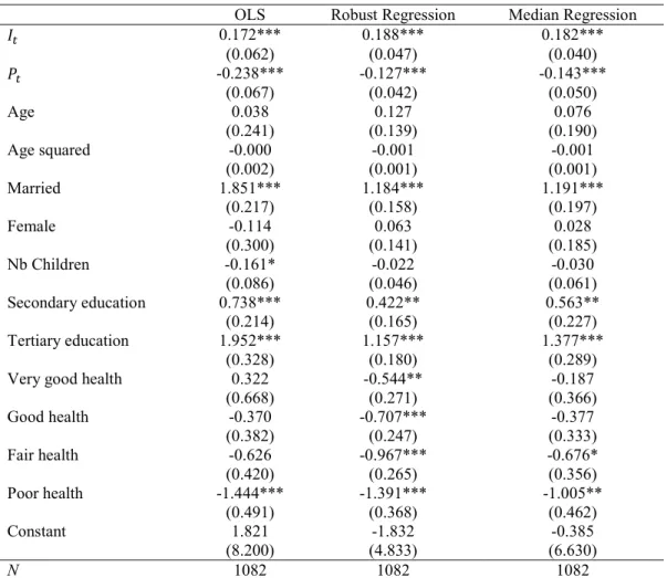
𝐼 0.172*** 0.188*** 0.182*** (0.062) (0.047) (0.040) 𝑃 -0.238*** -0.127*** -0.143*** (0.067) (0.042) (0.050) Age 0.038 0.127 0.076 (0.241) (0.139) (0.190) Age squared -0.000 -0.001 -0.001 (0.002) (0.001) (0.001) Married 1.851*** 1.184*** 1.191*** (0.217) (0.158) (0.197) Female -0.114 0.063 0.028 (0.300) (0.141) (0.185) Nb Children -0.161* -0.022 -0.030 (0.086) (0.046) (0.061) Secondary education 0.738*** 0.422** 0.563** (0.214) (0.165) (0.227) Tertiary education 1.952*** 1.157*** 1.377*** (0.328) (0.180) (0.289)

Very good health 0.322 -0.544** -0.187

(0.668) (0.271) (0.366) Good health -0.370 -0.707*** -0.377 (0.382) (0.247) (0.333) Fair health -0.626 -0.967*** -0.676* (0.420) (0.265) (0.356) Poor health -1.444*** -1.391*** -1.005** (0.491) (0.368) (0.462) Constant 1.821 -1.832 -0.385 (8.200) (4.833) (6.630) N 1082 1082 1082

Note: Robust standard errors in parentheses. In median regression, standard errors are based on 1,000 bootstrap replications. *_{p < 0.1,}**_{p < 0.05,}***_{p < 0.01.}

(29)

29

Table A2: Effect of public pension wealth on net non-pension wealth – Retired sample

𝐼 0.169*** 0.171*** 0.184*** (0.060) (0.047) (0.036) 𝑃 -0.222*** -0.121*** -0.144*** (0.073) (0.044) (0.050) Age -0.023 0.145 0.072 (0.276) (0.164) (0.215) Age squared 0.000 -0.001 -0.001 (0.002) (0.001) (0.002) Married 1.747*** 1.144*** 1.226*** (0.240) (0.167) (0.211) Female -0.246 -0.007 0.032 (0.329) (0.151) (0.202) Nb Children -0.184* -0.040 -0.048 (0.108) (0.054) (0.065) Secondary education 0.669*** 0.372* 0.589** (0.232) (0.191) (0.247) Tertiary education 1.827*** 1.113*** 1.356*** (0.372) (0.192) (0.253)

Very good health 0.658 -0.532* -0.112

(0.744) (0.301) (0.379) Good health -0.012 -0.630** -0.247 (0.364) (0.274) (0.338) Fair health -0.369 -0.892*** -0.581 (0.408) (0.300) (0.355) Poor health -1.034** -1.185*** -0.667 (0.491) (0.420) (0.519) Constant 3.660 -2.451 -0.597 (9.509) (5.768) (7.486) N 892 892 892

(30)

30

Table A3: Effect of public pension wealth on net non-pension wealth – Aged 60-75

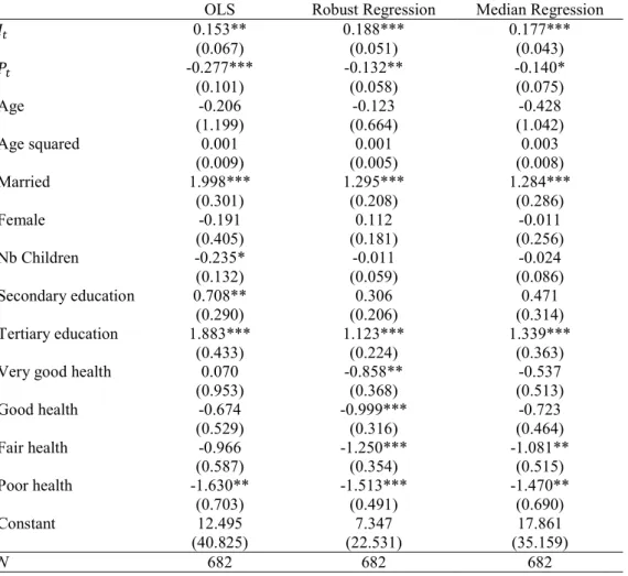
𝐼 0.153** 0.188*** 0.177*** (0.067) (0.051) (0.043) 𝑃 -0.277*** -0.132** -0.140* (0.101) (0.058) (0.075) Age -0.206 -0.123 -0.428 (1.199) (0.664) (1.042) Age squared 0.001 0.001 0.003 (0.009) (0.005) (0.008) Married 1.998*** 1.295*** 1.284*** (0.301) (0.208) (0.286) Female -0.191 0.112 -0.011 (0.405) (0.181) (0.256) Nb Children -0.235* -0.011 -0.024 (0.132) (0.059) (0.086) Secondary education 0.708** 0.306 0.471 (0.290) (0.206) (0.314) Tertiary education 1.883*** 1.123*** 1.339*** (0.433) (0.224) (0.363)

Very good health 0.070 -0.858** -0.537

(0.953) (0.368) (0.513) Good health -0.674 -0.999*** -0.723 (0.529) (0.316) (0.464) Fair health -0.966 -1.250*** -1.081** (0.587) (0.354) (0.515) Poor health -1.630** -1.513*** -1.470** (0.703) (0.491) (0.690) Constant 12.495 7.347 17.861 (40.825) (22.531) (35.159) N 682 682 682

(31)

31

Table A4: Effect of public pension wealth on net non-pension wealth – Men

𝐼 0.188*** 0.190*** 0.172*** (0.072) (0.050) (0.032) 𝑃 -0.268** -0.141** -0.155** (0.113) (0.056) (0.061) Age 0.081 0.085 0.164 (0.310) (0.200) (0.263) Age squared -0.001 -0.001 -0.001 (0.002) (0.001) (0.002) Married 1.500*** 0.963*** 1.025*** (0.348) (0.285) (0.286) Children -0.190 -0.022 0.004 (0.146) (0.063) (0.065) Secondary education 0.417 0.426* 0.449* (0.305) (0.239) (0.264) Tertiary education 2.086*** 1.286*** 1.467*** (0.571) (0.265) (0.296)

Very good health 1.400 -0.350 0.100

(1.131) (0.371) (0.452) Good health -0.516 -0.746** -0.352 (0.488) (0.336) (0.408) Fair health -0.371 -0.676* -0.297 (0.529) (0.356) (0.468) Poor health -1.477** -1.394*** -1.005* (0.637) (0.517) (0.571) Constant 0.395 -0.401 -3.392 (10.719) (7.000) (9.227) N 572 572 572

(32)

32

Table A5: Effect of public pension wealth on net non-pension wealth – Women

𝐼 -0.166 0.056 -0.065 (0.201) (0.165) (0.157) 𝑃 -0.008 -0.059 -0.040 (0.113) (0.099) (0.096) Age -0.007 0.205 0.129 (0.341) (0.204) (0.188) Age squared -0.000 -0.002 -0.001 (0.002) (0.001) (0.001) Married 2.050*** 1.310*** 1.320*** (0.266) (0.185) (0.197) Children -0.134 -0.030 -0.109 (0.087) (0.069) (0.066) Secondary education 1.192*** 0.503** 0.871*** (0.298) (0.223) (0.244) Tertiary education 1.933*** 1.160*** 1.552*** (0.348) (0.265) (0.262)

Very good health -0.866 -0.786* -0.890**

(0.590) (0.423) (0.401) Good health -0.255 -0.697* -0.752** (0.589) (0.394) (0.376) Fair health -0.997 -1.289*** -1.455*** (0.620) (0.408) (0.392) Poor health -1.557** -1.468*** -1.390*** (0.648) (0.542) (0.528) Constant 3.465 -4.188 -1.769 (11.595) (6.985) (6.511) N 510 510 510

(33)

33

Table A6: Effect of total public pension wealth at the household level

𝐼 -0.166 0.056 -0.065 (0.201) (0.165) (0.157) 𝑃 -0.008 -0.059 -0.040 (0.113) (0.099) (0.096) Age -0.007 0.205 0.129 (0.341) (0.204) (0.188) Age squared -0.000 -0.002 -0.001 (0.002) (0.001) (0.001) Married 2.050*** 1.310*** 1.320*** (0.266) (0.185) (0.197) Children -0.134 -0.030 -0.109 (0.087) (0.069) (0.066) Secondary education 1.192*** 0.503** 0.871*** (0.298) (0.223) (0.244) Tertiary education 1.933*** 1.160*** 1.552*** (0.348) (0.265) (0.262)

Very good health -0.866 -0.786* -0.890**

(0.590) (0.423) (0.401) Good health -0.255 -0.697* -0.752** (0.589) (0.394) (0.376) Fair health -0.997 -1.289*** -1.455*** (0.620) (0.408) (0.392) Poor health -1.557** -1.468*** -1.390*** (0.648) (0.542) (0.528) Constant 3.465 -4.188 -1.769 (11.595) (6.985) (6.511) N 510 510 510

(34)

34

Table A7: Expected replacement rate based pension wealth + constrained regression Expected

replacement rate Microsimulation

𝛽 ≠ 1 𝛽 = 1 𝛽 = 1 𝐼 -0.018** ₁ ₁ (0.007) 𝑃 -0.070 -0.600*** _-0.599*** (0.046) (0.063) (0.063) Age 0.070 -0.082 -0.060 (0.186) (0.244) (0.244) Age squared -0.001 0.001 0.000 (0.001) (0.002) (0.002) Married 1.170*** _1.901*** _1.922*** (0.196) (0.230) (0.229) Female -0.005 0.509* _0.520* (0.183) (0.299) (0.296) Nb Children -0.031 -0.163* _-0.157* (0.059) (0.091) (0.089) Secondary education 0.525** _0.613*** _0.582*** (0.242) (0.219) (0.220) Tertiary education 1.314*** _1.432*** _1.409*** (0.298) (0.329) (0.329)

Very good health -0.133 0.514 0.534

(0.345) (0.685) (0.683) Good health -0.332 -0.110 -0.125 (0.327) (0.398) (0.397) Fair health -0.642* _-0.594 _-0.587 (0.360) (0.457) (0.458) Poor health -0.995** _-1.323** _-1.328** (0.474) (0.518) (0.518) Constant -0.101 4.437 3.653 (6.478) (8.335) (8.313) N 1082 572 1082

(35)

35

Table A8: Effect of public pension wealth on net financial and real wealth – Full sample

OLS Robust regression Median regression

Financial

wealth Real wealth Financial wealth wealth Real Financial wealth wealth Real

𝐼 0.063 0.109*** 0.041*** 0.145*** 0.040*** 0.155*** (0.061) (0.036) (0.013) (0.034) (0.012) (0.025) 𝑃 -0.052 -0.186*** -0.023* -0.101*** -0.028** -0.099*** (0.051) (0.041) (0.014) (0.030) (0.014) (0.032) Age -0.217 0.255* -0.040 0.128 -0.083* 0.217* (0.165) (0.140) (0.042) (0.099) (0.046) (0.126) Age squared 0.001 -0.002* 0.000 -0.001 0.001* -0.002* (0.001) (0.001) (0.000) (0.001) (0.000) (0.001) Married 0.676*** 1.175*** 0.171*** 0.855*** 0.208*** 0.841*** (0.131) (0.148) (0.040) (0.108) (0.050) (0.138) Female -0.237 0.123 -0.030 0.121 -0.028 0.103 (0.208) (0.194) (0.039) (0.100) (0.041) (0.121) Nb Children -0.107 -0.054 -0.003 -0.018 -0.011 -0.011 (0.072) (0.042) (0.018) (0.031) (0.017) (0.036) Secondary education 0.222** 0.516*** 0.087* 0.277** 0.071* 0.363*** (0.109) (0.158) (0.047) (0.109) (0.043) (0.133) Tertiary education 1.009*** 0.943*** 0.205*** 0.757*** 0.336*** 0.839*** (0.272) (0.169) (0.059) (0.126) (0.069) (0.162)

Very good health 0.710 -0.388 0.070 -0.439** 0.101 -0.232

(0.559) (0.338) (0.082) (0.191) (0.130) (0.237) Good health 0.200 -0.570** 0.031 -0.603*** 0.065 -0.417* (0.199) (0.279) (0.075) (0.175) (0.093) (0.215) Fair health 0.145 -0.771*** -0.010 -0.740*** 0.009 -0.586** (0.228) (0.291) (0.074) (0.189) (0.084) (0.233) Poor health -0.227 -1.217*** -0.115 -1.008*** -0.092 -0.743** (0.291) (0.317) (0.100) (0.261) (0.104) (0.312) Constant 8.205 -6.384 1.721 -2.552 3.289** -5.842 (5.475) (4.893) (1.458) (3.417) (1.642) (4.316) N 1082 1082 1082 1082 1082 1082

(36)

36

Table A9: Effect of public pension wealth on net non-pension wealth – Adding covariates and interactions (Median regressions)

(1) (2) (3) (4) (5) (6) (7)

Risk

aversion characteristics Partner’s Inheritances educated Low educated High Married married Not

𝐼 0.173*** 0.181*** 0.185*** 0.248 0.176*** 0.195** _0.102 (0.038) (0.041) (0.037) (0.231) (0.049) (0.079) (0.156) 𝑃 -0.144*** -0.144*** -0.138*** -0.178 -0.207 -0.148** _-0.018 (0.054) (0.052) (0.049) (0.120) (0.131) (0.067) (0.112) Age 0.080 0.056 0.057 0.108 -0.158 0.161 0.365 (0.195) (0.199) (0.180) (0.303) (0.508) (0.240) (0.310) Age squared -0.001 -0.001 -0.001 -0.001 0.001 -0.001 -0.003 (0.001) (0.001) (0.001) (0.002) (0.004) (0.002) (0.002) Married 0.821*** 1.213*** 1.198*** 1.129*** 1.712*** - - (0.221) (0.201) (0.184) (0.260) (0.605) Female -0.121 0.002 0.061 -0.191 -0.198 0.100 -0.423 (0.209) (0.187) (0.173) (0.325) (0.482) (0.224) (0.370) Nb Children -0.026 -0.033 -0.023 -0.125 -0.074 -0.054 -0.030 (0.055) (0.061) (0.059) (0.078) (0.160) (0.074) (0.089) Secondary education 0.532** 0.547** 0.547** - - 0.529* _0.704** (0.215) (0.234) (0.218) (0.283) (0.312) Tertiary education 1.167*** 1.357*** 1.293*** - - 1.473*** _1.156*** (0.231) (0.280) (0.244) (0.327) (0.418) Very good health -0.488 -0.184 -0.198 -0.147 -1.363* -0.103 -0.912 (0.344) (0.378) (0.350) (0.659) (0.812) (0.411) (0.699) Good health -0.661** -0.387 -0.390 -0.184 -1.524* -0.321 -1.123* (0.308) (0.343) (0.319) (0.546) (0.785) (0.371) (0.637) Fair health -0.902*** -0.692* -0.685** -0.445 -1.874** -0.563 -1.546** (0.333) (0.364) (0.346) (0.562) (0.858) (0.432) (0.635) Poor health -1.314*** -1.035** -0.964** -0.827 -2.156* -1.123* _-1.855** (0.455) (0.476) (0.438) (0.704) (1.173) (0.595) (0.740) Risk averse -0.868*** - - - - (0.179) Partner work - 0.201 - - - - - (0.591) Partner education - 0.427 - - - - - (0.365) Inheritances - - 0.604 - - - - (0.381) Constant 0.408 -0.122 0.194 -1.658 9.999 -2.104 -10.036 (6.808) (6.952) (6.240) (10.726) (17.527) (8.265) (10.795) N 1082 1082 1082 265 314 794 288

Note: Robust standard errors in parentheses. Standard errors are based on 1,000 bootstrap replications. *_{p <}