Département de génie civil
LES EFFETS DU CHANGEMENT CLIMATIQUE SUR LA PLUIE MAXIMALE PROBABLE ET LA CRUE MAXIMALE PROBABLE AU QUÉBEC
CLIMATE CHANGE IMPACT ON PROBABLE
MAXIMUM PRECIPITATION AND PROBABLE
MAXIMUM FLOOD IN QUÉBEC
Thèse de Doctorat Spécialité: génie civil
Hassan ROUHANI
Jury: Robert LECONTE (directeur)
Faisal HOSSAIN (University of Washington) Norman JONES (Bishop’s University)
Jay LACEY (Université de Sherbrooke)
iii
Quand la température atmosphérique à la surface a des augmentations en raison du réchauffement climatique mondial, la capacité des niveaux atmosphériques inférieurs à contenir de la vapeur d’eau s’élève. Ceci peut influencer les précipitations et les inondations. C’est pourquoi le réchauffement mondial conduit au changement climatique. Les précipitations extrêmes et les inondations extrêmes peuvent potentiellement subir des changements, à savoir, la précipitation maximale probable (PMP) et la crue maximale probable (CMP). Cette recherche vise à analyser les influences du changement climatique sur la PMP et la CMP dans trois bassins versants avec différentes conditions climatiques à travers la province de Québec, Canada. Les bassins versants sont situés dans le sud, le centre et le nord du Québec. Ils ont été sélectionnés d’une manière qui reflète la diversité du climat à travers le Québec.
Afin d'étudier les conditions du changement climatique, les sorties du modèle régional canadien du climat (MRCC) ont été utilisées. Cette base de données couvre un horizon de temps à partir de 1961 jusqu'à 2100. Les données comprennent la précipitation quotidienne, la température, l'humidité spécifique et l’énergie potentielle de convection disponible (EPCD). Ces données ont été utilisées pour estimer la PMP. La méthode de l’Organisation Météorologique Mondiale (OMM) a été adaptée pour estimer les valeurs de la PMP dans des conditions de changements climatiques. L'eau précipitable centennale (W100) a été choisie comme une limite supérieure de l'eau précipitable pour déterminer le rapport de maximisation. Les séries chronologiques pour estimer W100 ont été établies à partir de valeurs annuelles maximales d'eau précipitable qui sont associées à des valeurs de variables atmosphériques similaires à l'événement qui doit être maximisé. Les variables atmosphériques utilisées dans cette recherche sont la température atmosphérique à la surface et l'EPCD. Cette méthode ne nécessite pas de fixer une limite supérieure au rapport de maximisation et est donc plus propice à la détermination de la PMP dans un contexte des changements climatiques.
La PMP résultante a été utilisée pour forcer un modèle hydrologique distribué afin d’estimer la CMP. Les valeurs de la PMP et de la CMP ont été estimées en trois horizons de temps: le passé récent, les futurs proches (2030) et lointains (2070). Dans les régions où la fonte des neiges joue un rôle clé dans le cycle hydrologique annuel, les crues printanières en climat actuel correspondent habituellement au débit maximum annuel. La PMP et la CMP ont cependant été analysées séparément en deux saisons: l'été-automne (sans neige) et l'hiver-printemps (accumulation et fonte de neige) pour évaluer l’impact des changements climatiques sur la saisonnalité de ces événements extrêmes. La plus grande valeur obtenue a été identifiée comme la PMP / CMP annuelle. La CMP d’été-automne a été estimée par l'insertion de la PMP pour chaque jour de l'horizon de temps de simulation. Par conséquent, toutes les conditions possibles d'humidité du sol avant l’événement de la PMP ont été incluses. En conséquence, une distribution des valeurs de CMP basées sur différentes conditions initiales (niveaux d'humidité du sol) a été obtenue. La CMP d’hiver-printemps a été estimée en insérant la valeur de PMP à la fin d'une période de fonte et une accumulation de neige extrême.
Nos résultats montrent que dans le sud et le nord du Québec, la CMP a toujours lieu à la fin de la saison hiver-printemps lorsque l’accumulation de neige est maximale. Aussi, la PMP et la CMP au sud du Québec devraient diminuer, mais la tendance au centre et au nord du Québec serait inversée. Dans le centre et le nord, la CMP augmente de 22 et 21%, respectivement, à la fin du 21e siècle alors que pour la même période, CMP aurait une réduction de 13% dans le
iv
sud du Québec. La CMP annuelle de ces bassins versants se produit dans la saison hiver-printemps dans trois horizons temporels.
Mot- clés : PMP, CMP, changements climatiques, Québec.
ABSTRACT
As atmospheric temperatures at the Earth’s surface increase due to global warming, the capacity of lower atmospheric levels to hold water vapor rises and thus, precipitations and floods will be influenced. In turn, extreme precipitation and flood events are subject to potential modifications under climate change, namely, Probable Maximum Precipitation (PMP) and Probable Maximum Flood (PMF). This research aims at analyzing climate change influences on PMP and PMF in three watersheds with different climatic conditions across the province of Québec, Canada. The watersheds are located in the south, center and north of the province. They have been selected in a manner which reflects climate diversity across Québec. In order to study climate change conditions, the data output of the Canadian Regional Climate Model (CRCM) was used. This database covers a time horizon from 1961 up to 2100 and includes daily precipitation, temperature, specific humidity and Convective Available Potential Energy (CAPE). These data were used to estimate PMP. The World Meteorological Organization (WMO) method was adapted to estimate PMP values under climate change conditions. The 100-year return period precipitable water (W100) was selected as an upper limit of precipitable water in establishing maximization ratio. The time series for estimating W100 was established from annual maximum precipitable water values that have similar atmospheric variables of the event to be maximized. The atmospheric variables used in this research were atmospheric temperature at the Earth’s surface and CAPE. This method does not require setting any upper bound limit to the maximization ratio and is therefore more amenable to calculate the PMP in a climate change context.
The PMP was used to run a distributed hydrological model to estimate PMF. PMP and PMF values were estimated in three 45-year time horizons: recent past (centered on 1985), near future (2030) and far future (2070). In regions where snowmelt plays a key role in the annual hydrological cycle, winter-spring flooding could be the major discharge. Consequently, PMP and PMF were separately analyzed in two seasons: summer-fall (snow-free) and winter-spring (snow accumulation and melt). The largest value obtained was identified as the all-season PMP/PMF. Summer-fall PMF was estimated by inserting the PMP in each day of the simulated time horizon. Therefore, all soil moisture conditions prior to PMP occurrence were included. Accordingly, a distribution of PMF values based on different initial conditions (soil wetness levels) was obtained. Winter-spring PMF was estimated by inserting the PMP value at the end of a warm melting period and for an extreme snow accumulation.
Our results show that the PMF of three watersheds would occur in the winter-spring season in current and future climate projections. Furthermore, all-season PMP and PMF in southern Québec would decrease, but trends in central and northern of Québec would be reversed and the PMP and PMF would increase in projected climate conditions. In the center and north of Québec, the PMF would increase by 25 and 23% respectively, at the end of the 21st century. For the same period, PMF would have a reduction of 25% in the south of Québec. Of the three watersheds, the PMF always occurs at the end of winter-spring season when the snow accumulation is the greatest.
v
REMERCIEMENTS
My utmost gratitude goes to the director of this research, Professor Robert Leconte. I would like to thank him for his support, for motivating me during these years and for trusting me in my research. His professional advice has helped me not only in my research career, but also in other aspects of my life.
In addition to my advisor, I would like to thank the jury members of my research proposal, Professor Jay Lacey, Professor Norman Jones and Professor Faisal Hossain for their valuable comments.
I would like to thank Dr. Trudel, Dr. Haguma and all of my fellow researchers in Le Groupe de Recherche sur l'EAU de l'Université de Sherbrooke (GREAUS) for their insightful scientific discussions.
I also wish to thank the Ouranos consortium for providing the required data of this research. I express my deep gratitude to my family, who has always been concerned about me and my life. I thank my kind parents for their support, my beloved sister and her family for motivating and encouraging me and my dear brother for inspiration and scientific discussions. I also thank my precious in-laws for their wonderful reassurance and support.
Finally, I would like to thank Leila, my wife, from the bottom of my heart, for her patience, for her patience and for her patience.
vi
TABLE DES MATIÈRES
RÉSUMÉ ... iii
REMERCIEMENTS ... v
TABLE DES MATIÈRES ... vi
LISTE DES FIGURES ... viii
LISTE DES TABLEAUX ... x
LISTE DES SYMBOLES ... xi
LISTE DES ACRONYMES ... xii
CHAPITRE 1 Introduction ... 1
1.1 Why are PMP and PMF important? ... 2
1.1.1 Use of PMP and PMF in Canada ... 2
1.1.2 Use of PMP and PMF in the USA ... 3
1.1.3 Impacts of climate change on PMP and PMF ... 4
1.2 Research question ... 5
1.3 Thesis plan ... 6
CHAPITRE 2 Literature review ... 7
2.1 PMP ... 8
2.1.1 PMP estimation using statistical methods ... 8
2.1.2 PMP estimation using deterministic approaches ... 9
2.1.3 PMP estimation using numerical methods ... 14
2.1.4 PMP and climate change ... 16
2.2 Probable Maximum Flood (PMF) ... 19
2.2.1 Approaches to estimate PMF ... 20
2.2.2 PMF under climate change conditions ... 21
2.3 Summary ... 23 CHAPITRE 3 Methodology ... 24 3.1 Research assumptions ... 26 3.2 Watersheds ... 28 3.2.1 Chaudière watershed ... 28 3.2.2 Moisie watershed ... 29
3.2.3 Great Whale watershed ... 31
3.3 Data ... 32
3.3.1 Climate model selection ... 34
3.3.2 Validity of the CRCM output data over the study sites ... 36
3.4 PMP estimation method ... 43
3.5 Hydrological model ... 49
3.6 Hydrological model calibration and validation ... 50
3.7 PMF estimation ... 53 CHAPITRE 4 Paper 1 ... 59 4.1 Abstract ... 60 4.2 Introduction ... 60 4.3 Methodology ... 63 4.3.1 Data ... 63 4.3.2 Watersheds ... 65 4.3.3 PMP approach... 68 4.4 Results ... 73
vii 4.5 Discussion ... 78 4.6 Conclusion ... 84 CHAPITRE 5 Paper 2 ... 85 5.1 Abstract ... 86 5.2 Introduction ... 86
5.3 Probable Maximum Flood (PMF) and climate change impacts ... 88
5.4 Methodology ... 90 5.4.1 Watersheds ... 90 5.4.2 Data ... 93 5.4.3 Hydrological modeling ... 95 5.4.4 PMP ... 97 5.4.5 PMF ... 100 5.5 Results ... 102
5.5.1 Climate change projection ... 102
5.5.2 Summer-Fall floods ... 103
5.5.3 Winter-Spring floods ... 106
5.6 Discussion ... 109
5.7 Conclusion ... 114
CHAPITRE 6 Discussion ... 116
6.1 What was the idea of the thesis? ... 117
6.2 CRCM vs. observation ... 117
6.3 What is uncertainty of the results? ... 120
CHAPITRE 7 Conclusion ... 121
7.1 Contribution ... 122
7.2 Recommendation for future work... 124
Appendix ... 126
viii
LISTE DES FIGURES
Figure ( 2-1): An imaginary atmospheric control volume ... 10
Figure ( 2-2): subdivision of the province of Québec into regions according to origin of storms [CEHQ and SNC-Lavalin, 2003]. Climatological regions are also shown in the figure... 12
Figure ( 2-3): Trend of maximum precipitable water in southern Québec in the month of August from 1960 to 2100 [Rousseau et al., 2014] ... 17
Figure ( 3-1): General flow-chart of methodology used in this research. ... 25
Figure ( 3-2): The geographical situation of watersheds under study in this research. ... 30
Figure ( 3-3): Monthly average hydrographs for the three watersheds of this study. ... 32
Figure ( 3-4): Earth’s atmosphere system showing an atmospheric circulation [Stull, 2000]. .. 33
Figure ( 3-5): Global average of surface warming for different scenarios. Shading denotes ±1 of standard deviation of models annual average. The orange line is a reference, for which the concentration is kept constant. The grey bars at the right indicate the best estimate (solid line in each bar) and the likely range for SRES scenarios [IPCC, 2007]. ... 35
Figure ( 3-6): Three watersheds with CRCM tiles covering the area of interest. Upper left: Chaudière, upper right: Moisie, bottom: Great Whale. ... 36
Figure ( 3-7): comparison between CRCM output and observation data at three watersheds: bottom: Chaudière, middle: Moisie and top: Great Whale ... 38
Figure ( 3-8): comparison of normalized root mean square error of precipitation between aft and afx in each pixel of watersheds ... 38
Figure ( 3-9): Bias removal performance at Chaudière watershed for the recent past time horizon. ○, □ and ◊ represent biased data, bias removed afx data and observation, respectively. ... 40
Figure ( 3-10): Trend in maximum precipitable water for the month of August in one CRCM tile of each study watershed ... 42
Figure ( 3-11): Convective lifting process. P and T represent pressure and temperature, respectively [Stull, 2000]. ... 46
Figure ( 3-12): The relation between CAPE and depth of large precipitation events at Chaudière watershed. Vertical axis is CAPE in [kj/kg] and horizontal axis is rainfall depth in [cm]. Each box describes a large (as described in the text) precipitation event, and each dot represent a CRCM tile (as depicted in the Figure ( 3-6)). ... 47
Figure ( 3-13): Result of calibration at Chaudière. ... 52
Figure ( 3-14): Result of calibration at Moisie. ... 52
Figure ( 3-15): Result of calibration at Great Whale. ... 53
Figure ( 3-16): Generalized isohyetal map of a PMP [WMO, 2009] ... 57
Figure ( 4-1): Location of the three watersheds in this study in the province of Québec, Canada. ... 66
Figure ( 4-2): Three watersheds with CRCM tiles covering the area of interest. Upper left: Chaudière, upper right: Moisie, bottom: Great Whale. ... 72
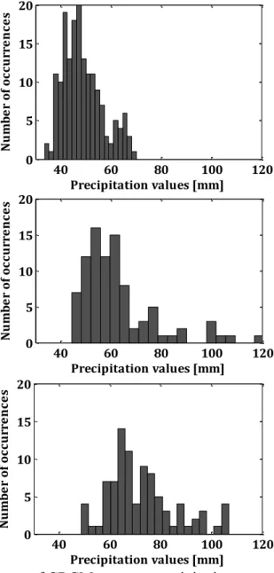
Figure ( 4-3): Histograms of CRCM extreme precipitation events which were used in maximization process of PMP estimation in each tile of three watersheds, upper: Great Whale, middle: Moisie and bottom: Chaudière. ... 74
Figure ( 4-4): Probability plot of annual maximum precipitable water using the traditional method and the new approach at three watersheds, upper: Great Whale, middle: Moisie and bottom: Chaudière. “◊”, “” and “” represent temperature-CAPE filter, temperature filter and traditional approaches, respectively. ... 75
ix
Figure ( 4-5): Variation of the maximization ratio (left column) and PMP (right column) in the watersheds calculated from the maximization ratios obtained from left panels (no upper limit modifications was imposed), top: Great Whale, center: Moisie, down: Chaudière. ... 76 Figure ( 4-6): Example of temperature drop during a CRCM rainstorm event in the Chaudière watershed. ... 80 Figure ( 4-7): Spatial distribution of maximization ratio, the events produced PMP and PMP values at three watersheds. ... 82 Figure ( 5-1): Location of the three watersheds in this study in the province of Québec, Canada. ... 91 Figure ( 5-2): Average (mean of daily values between 1960-2005) hydrograph for the three watersheds in the study. ... 93 Figure ( 5-3): Observed and simulated average hydrographs for the 1980-1991 time period for the Chaudière watershed. ... 97 Figure ( 5-4): Study watersheds with CRCM tiles covering the area of interest. Upper left: Chaudière, upper right: Moisie, bottom: Great Whale. ... 100 Figure ( 5-5): Rate of precipitation regime change to temperature regime change. “○”, “□” and “◊” represent Chaudière, Moisie and Great Whale, respectively. Solid/hollow symbols
represent near/far future. ΔP/P is mean daily seasonal precipitation difference between future and control period over control period. ΔT is mean daily seasonal temperature difference between future and control period. ... 103 Figure ( 5-6): Empirical cumulative distribution function of PMF values in the Great Whale watershed for the 2070 horizon. ... 104 Figure ( 5-7): Annual maximum SWE values from which SWE100 is calculated in each time horizon for the Great Whale watershed. ... 108
x
LISTE DES TABLEAUX
Table ( 2-1): PMP conversion factors in the region A,G [CEHQ and SNC-Lavalin, 2003]. Grey
boxes: spring, white boxes: summer-fall ... 12
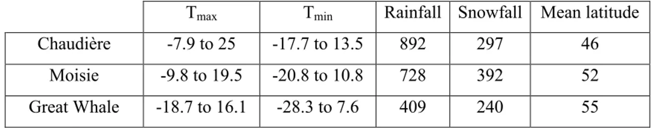
Table ( 3-1): Average latitude, daily maximum and minimum temperature for the coldest and warmest month (oC) and total annual snowfall and rainfall (mm) at three watersheds (1981-2010) time horizon. ... 31
Table ( 3-2): comparison between observed and CRCM simulated 100-year precipitable water values at Sept-Îles weather station [Chow and Jones, 1994]. ... 41
Table ( 3-3): comparing the largest events (mm) simulated by CRCM (aft and afx) averaged over the watersheds versus observational data (NLWIS) ... 42
Table ( 3-4): comparing the number of events exceeding 25 mm (averaged over the watershed) produced by CRCM (afx) versus observation. ... 43
Table ( 3-5): Summer-fall and spring description in Québec based on geographical situations. ... 49
Table ( 3-6): Summary of considerations that led to selecting the SWAT model. ... 50
Table ( 4-1): Physiographic and hydrographic characteristics of the watersheds. ... 67
Table ( 4-2): Climate characteristics of the watersheds. ... 68
Table ( 4-3): Summer-fall description in Québec based on geographical locations. ... 71
Table ( 4-4): Mean and standard deviation of precipitation events at three watersheds. ... 73
Table ( 4-5): Median and variability of maximization ratios for the three watersheds. Trad stands for traditional method, T-filter and TC-filter represent temperature and temperature-CAPE filter methods, respectively. ... 77
Table ( 4-6): Median and 95th percentile of PMP (mm) for three watersheds estimated using three methods. In parentheses, the maximization ratio of the traditional method was not allowed to exceed 2. ... 78
Table ( 5-1): Physiographic and climatic conditions (including 100-year return period rainfall and flood) of the watersheds under study [CEHQ, 2015b; Environment Canada, 2015]. ... 92
Table ( 5-2): Nash-Sutcliffe for the watersheds under study. ... 96
Table ( 5-3): Summer-fall and winter-spring description for Québec based on geographical location. ... 99
Table ( 5-4): Summer-fall PMF and PMP for three watersheds and three time horizons. JJ stands for June-July, AS for August-September and ON for October-November. ... 104
Table ( 5-5): Winter-spring PMF (m3/s), PMP (mm) and SWE100 (mm) for three watersheds and three time horizons. DJ stands for December-January, FM for February-March and AM for April-May. ... 106
Table ( 5-6): Mean of T100 (oC) time series during melting period for three watersheds and three time horizons. ... 108
Table ( 5-7): Comparison between results from this study and results for an adjacent watershed. ... 110
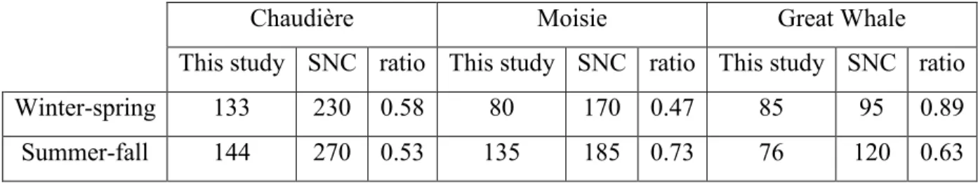
Table ( 5-8): Comparison between results from this study and from SNC [CEHQ and SNC-Lavalin, 2004]. ... 111
Table ( 5-9): Extreme events (mm) and maximization ratio in each time horizon producing PMP before being maximized in the three watersheds. ... 114
xi
LISTE DES SYMBOLES
Symbol Definition
100 100-year return period event
E Total energy
F Wind speed
Ft Transposition adjustment factor
g Gravitational acceleration
h Altitude
k Shape parameter of statistical distribution
K Frequency factor
m mass
P Pressure
pw Saturation vapor pressure
Q Specific humidity Qm Modeled runoff Qo Observed runoff r Maximization ratio s Scaling factor S Standard deviation t Time T Temperature U Internal energy W Precipitable water
Mean of annual maximum values
λ Scale parameter of statistical distribution
ψ Location parameter of statistical distribution
xii
LISTE DES ACRONYMES
Acronym Definition
CAPE Convective Available Potential Energy CGCM Canadian Global Coupled Model CLASS Canadian LAnd Surface Scheme CRCM Canadian Regional Climate Model
DDF Degree-Day Factor
GW Great Whale
GCM General Circulation Model GEV General Extreme Value
GHG Greenhouse gas
IDF Intensity-Duration-Curve
IPCC Inter-governmental Panel on Climate Change
LAM Limited Area Model
LFC Level of Free Convection LOCI Local Intensity
LULC Land use land cover
NLWIS The National Land and Water Information Service NS Nash-Sutcliffe criterion
PDF Probable Density Function PDS Partial Duration Series PMF Probable Maximum Flood PMP Probable Maximum Precipitation
PMS Probable Maximum Storm
Pobs Observed Precipitation RCM Regional Climate Model
RH Relative Humidity
SAT Saturation
SCHADEX Simulation Climato-Hydrologique pour l’Appréciation des Débits EXtrêmes SWAT Soil Water Assessment Tool
SWE Snow Water Equivalent Tmax Maximum Daily Temperature Tmin Maximum Daily Temperature USA United States of America
WDT Wet Day Threshold
WMF Wind Maximization Factor
1
1.1 Why are PMP and PMF important?
1.1.1
Use of PMP and PMF in CanadaThe Probable Maximum Flood (PMF) is defined as the largest flood that can reasonably occur [Ely and Peters, 1984]. This extreme flood theoretically happens when critical meteorological conditions occur simultaneously along with severe hydrological conditions. The PMF is typically computed using a hydrological model forced with critical meteorological conditions. In the province of Québec, for example, PMF can be the result of an extreme rainfall event over saturated soil or of a combination of an extreme precipitation event and an extreme snowpack during the spring melt season. The extreme rainfall event chosen is typically the Probable Maximum Precipitation, or PMP. According to the World Meteorological Organization (WMO), the PMP is defined as “the greatest depth of precipitation for a given
duration meteorologically possible for a design watershed or a given storm area at a particular location at a particular time of year, with no allowance made for long-term climatic trends” [WMO, 2009].
PMP in the province of Québec, Canada, has been estimated for different watersheds since 1960’s [Perrier, 1968]. Since then, a number of studies developed and applied methods to estimate PMP and PMF e.g. [Beauchamp et al., 2013; Debs et al., 1999; Hydro-Québec and
SNC-Shawinigan, 1992]. Among the studies that estimated PMP values in the Québec
watersheds, one of the most comprehensive is a report produced by SNC-Lavalin, an engineering firm, in collaboration with the Centre d’expertise hydrique du Québec1 (CEHQ), a provincial agency part of the Ministère du Développement durable, de l’Environnement et de la Lutte contre les changements climatiques (MDDELCC) [CEHQ and SNC-Lavalin, 2003]. CEHQ’s mission is to manage the Québec water regime securely, equitably and in a sustainable development perspective. In that report, PMP values were estimated over most of the Québec territory using the moisture maximization approach recommended by WMO [WMO, 1986]. In this method, PMP values are estimated by scaling large observed events. The scaling process includes raising atmospheric moisture of a large observed storm towards an upper bound. A proxy of atmospheric moisture is surface dew point temperature and an upper bound to this can be the maximum value recorded at location and time of PMP estimation.
1 Following a restructuring process in 2016, the various units of the CEHQ have been incorporated into the
PMP and PMF are important to calculate because they are used in designing hydraulic structures, such as dams and spillways. For example, the government of Québec enforced the Dam Safety Act in 2002 [Gouvernement du Québec, 2015a]. According to this Act, dam owners are responsible for assuring the safety of the dams. This Act also defines design criteria for dams. Large dams whose failure results in death or severe financial loss must be constructed based on the PMF. It is interesting to note that the Dam Safety Act was created following the so-called Saguenay Flood, which occurred in 1996 in the Saguenay region of Québec. The flood caused 800 million CAD of damage and 10 deaths [Milbrandt and Yau, 2001]. The flood was 8 times larger than the 100-year return period flood. It was triggered by an extreme summer precipitation in a region where there were some deficiencies in the maintenance of hydraulic structures. Furthermore, a reservoir breach worsened these conditions [Lapointe et al., 1998]. The Saguenay Flood also prompted the Québec Government to create the CEHQ.
It is also worth mentioning that other Canadian provinces follow similar PMP and PMF estimation practices as well. PMP and PMF values are estimated for regional hydraulic structures safety in other Canadian provinces, such as British Colombia (BC), Alberta, Saskatchewan [Abrahamson and Pentland, 2010; Hopkinson, 1999; Verschuren and Wojtiw, 1980]. In all these studies, PMP and PMF values are being estimated following the WMO approach using available observed record of storms and atmospheric moisture in the weather stations.
1.1.2
Use of PMP and PMF in the USAUse of PMF as a dam design criterion has a long history in the USA. Back in 1938, the maximum flood flow was recommended for designing of dams whose failure could cause risk of life [National Resources Committee, 1938]. Later, following a Task Force on Spillway Design Floods in 1956, a paper was published that endorsed the same suggestion [Snyder, 1964]. This approach was then used in numerous literature see [Bureau of Reclamation, 1987] and led to producing documents upon request of various federal agencies to provide PMP/PMF for different regions of the USA. Examples are the documents produced by National Weather Service for estimating PMP in California, Alaska, US East of the 105th Meridian, among others [Corrigan, 1999; Francis and John, 1983; Schreiner and Riedel, 1978]. Despite the extensive use of this concept, there has been some controversy on use of
this method. While some researchers recommend of securing dams with PMFs, there are oppositions to this idea [Graham, 2000]. The main issue lies in fortifying existing dams as they have not been built using PMF values. On one hand, there are researchers/practitioners who believe in maximum safety without assigning a dollar value to los of life. Others recommend that the focus be on the careful investigation of safety issues along with consideration for economic resources, including groups that believe that retrofit ting dams is wasteful e.g. [Resendiz-Carillo and Lave, 1987].
In spite of these arguments, PMF still serves as a design standard; however, some improvements in the estimation methods have been suggested. Recently, taking advantage of numerical weather models, a more physically based approach to estimate PMP, and in turn, PMF was developed [Abbs, 1999; Ohara et al., 2011; Stratz and Hossain, 2014]. This approach also allows studying PMP under regional land use and land cover changes [Yigzaw et
al., 2012; Yigzaw et al., 2013]. As well, a number of studies focused on the potential influence
of global climate change on PMP e.g. [Kunkel et al., 2013], and PMF e.g. [Beauchamp et al., 2013] accordingly.
1.1.3
Impacts of climate change on PMP and PMFThe province of Québec possesses significant amounts of freshwater. There are indications that global warming has affected the regional climate and, more specifically, the precipitation and temperature regimes across the province. For example, annual mean temperature in areas of Québec has increased by 1.8 oC over the last 50 years [Yagouti et al., 2008]. Moreover, projections of maximum summer-fall discharge under climate change conditions in northern Québec indicate that floods would most likely follow an increasing trend. As it is expected, the trend for larger floods would be more significant [CEHQ, 2015a]. A study by Mailhot et al. (2010), based on statistical analyses of climate model outputs, reported that annual maximum daily rainfall in future climate conditions across Canada (including Québec) would intensify [Mailhot et al., 2010]. In southern Québec, for example, the study shows that the return period for short duration rainfall events (2 hours and 6 hours) would halve in future climates [Mailhot et al., 2007].
Recent research report that summer-fall PMP in southern/central Québec would increase/decrease in transition from the recent past to the near future (2001-2040) [Beauchamp
change conditions [Beauchamp et al., 2013; Rousseau et al., 2014], it is necessary for dam owners to make sure that existing structures are also secure for future climate conditions. As well, new structures must be designed based on hydrological extremes taking into account future climate conditions.
A number of approaches have been proposed to investigate climate change impacts on PMP. One such approach is to extrapolate the observed trends of climatic variables into the future and to analyze the potential impacts on PMP e.g. [Clark, 1987]. This approach, however, does not allow capturing the possible non-linear behavior of the extrapolated variable. Another method of studying PMP in a changing climate is by using climate models outputs. These models produce future climate projections based on possible greenhouse gas (GHG) emission scenarios. Output of these models are becoming more and more available and therefore, can be used to study climate change effects on PMP e.g. [Beauchamp et al., 2013]. Finally, numerical weather models have been recently used to investigate the impacts of anthropogenic activities on the local and regional climate, and more specifically on extreme precipitation events such as the PMP. Anthropogenic activities include land use and land cover (LULC) changes such as irrigation and reservoirs [Yigzaw et al., 2012]. Although these studies can be considered as climate change impact studies, using climate models to study the combined influence of LULC and anthropogenic greenhouse gas (GHG) emissions on PMP in a way similar as with weather models remains a challenging task.
1.2 Research question
Québec will likely be facing climate change conditions [Vescovi et al., 2009]. This may influence the regime of extreme precipitation and floods across Québec. Considering that Québec takes advantage of water resources with different usages and because of numerous hydraulic structures already installed across the province, a reevaluation of safety and security of the dams is necessary. Therefore, in this study, the influence of future climate change conditions on the PMP and PMF in different regions of Québec will be analyzed. The influence of climate change on the hydrological regime of watersheds is site-specific; consequently, three different watersheds were selected for study. These watersheds are located in the southern, northern and central areas of Québec and each are characterized by different climatic regimes and physiographic characteristics. This will allow for the investigation of the influence of climate change conditions at different latitudes with diverse watershed climatic
and physiographic characteristics. Accordingly, the main objectives of this research can be stated as:
I) to develop and test a method to investigate the impact of climate change on daily PMP
II) using the approach in I), to investigate the influence of climate change on the summer-fall and winter-spring daily PMP and corresponding PMF of northern watersheds where snow accumulation and melt play a significant role in the overall hydrological regime.
1.3 Thesis plan
A literature review on state-of-the-art research in PMP, PMF and climate change impacts on hydrological regimes is presented in Chapter 2.
The proposed methodology for computing PMP and PMF is explained in Chapter 3. The methodology covers a description of the data used, a presentation of the watersheds, the approach for estimating PMP and the hydrological modeling steps in this research. Finally, the techniques which were utilized in estimating summer-fall and winter-spring PMF estimations are outlined.
Two research articles based on the findings of this research are presented in Chapters 4 and 5. The first article (Chapter 4) contains the results of the methodology that was developed for estimating PMP in the context of climate change. The second article (Chapter 5) presents and analyses the results of investigating the influence of climate change on PMF using the PMP approach developed in this thesis. Further analyses and discussions follow in Chapter 6. Lastly, concluding remarks from the results of this thesis as well as suggestions for further work are outlined.
7
This section outlines past research studies devoted to analyses of PMP and PMF and also for assessing the potential influence of climate change on precipitation and flooding. In this section, the concepts of PMP and PMF are introduced along with their calculation methods.
2.1 PMP
The concept of PMP, which is introduced in Chapter 1, does not consider a return period. Although the risk of occurrence always remains [Koutsoyiannis, 2004], the probability of occurrence of exceeding an event is theoretically nil [Dumas, 2006]. PMP, as the greatest
depth of precipitation [WMO, 2009], implies maximizing precipitation events. Hence, a
maximization method should be applied in order to obtain PMP. There are three main methods for deriving PMP from datasets of precipitation, and which are introduced in the following sections.
2.1.1
PMP estimation using statistical methods
Following statistical analyses on thousands of weather stations mostly located in the USA, Hershfield suggested in the 1960’s adapting the following frequency equation for PMP estimation, which was originally proposed by Chow for analyzing flood events [Chow, 1951]:
(2-1)
In equation ( 2-1), X is the magnitude of a hydrological event (e.g. rainfall) of a given duration at a particular probability level, is the mean of the time series of annual maxima, K is a frequency factor and is the standard deviation of the series [Hershfield, 1981]. In order to estimate PMP from equation ( 2-1), Hershfield adjusted the K factor to produce a precipitation event for which the return period is theoretically infinite.
WMO recommends this PMP estimation approach for small size watersheds. This approach has been used frequently because of its simplicity and ease of calculation (e.g. [Jothityangkoon et al., 2013; Rezacova et al., 2005]). To some extent, most of the recent PMP estimations using this approach have modified the original method of Hershfield. For instance, in Czech Republic [Rezacova et al., 2005], Spain [Casas et al., 2011], Malaysia [Desa et al., 2001] and India [Rakhecha and Clark, 2000], the Hershfield approach was used to estimate PMP but frequency factors used in the estimations were not the original frequency factors recommended by Hershfield, as these values were retrieved from observations mostly located in the USA. Instead, they used K factors more adapted to these countries.
A main advantage of statistical approaches such as Hershfield’s method is their ease of application. However, a disadvantage of such approaches is that the K value of equation ( 2-1) is sensitive to record length [Koutsoyiannis, 1999]. Therefore, PMPs are subject to change as historical records become more complete. Another drawback of statistical approaches is that they are not physically based; in other words, they do not consider the physics behind extreme rainfall generation. A physically based approach should be more amenable to generate realistic extreme rainfall events. Finally, this method is not easily amenable to climate change impact studies as they depend heavily on climate models daily precipitation output which as well known to show biases.
This method has been used in a number of studies to estimate PMP under future climate conditions e.g. [Afrooz et al., 2015; Jothityangkoon et al., 2013]. However, it should be noted that statistical PMP estimation methods rely on observed observations. Therefore, the use of such approaches to estimate PMP in a future climate relies exclusively on simulated precipitation, e.g. from climate models, and therefore do not explicitly include information on the physics of extreme rainfall events.
2.1.2 PMP
estimation
using
deterministic
approaches
The purpose of maximizing a rainstorm event is to achieve the largest possible depth of rainfall. Unlike the statistical method, the deterministic method (sometimes called moisture maximization approach as well) is based on the physical phenomena which take place upon extreme precipitation. The idea of this method is to maximize extreme observed rainfall events. In other words, large storms are selected and, subsequently, maximized according to their characteristics. Therefore, the logic behind the deterministic approach is in estimating the potential upper bound of the precipitation amount by maximizing the atmospheric moisture, which is related to storm formation and development [Rakhecha and Singh, 2009]. The concept of PMP estimation using moisture maximization method can be visualized through the mass balance equation applied to an imaginary atmospheric control volume [Chen and
Bradley, 2003], as seen in Figure ( 2-1). In the PMP process, it is assumed that the winds
remain favorable (in terms of feeding the storm with precipitable water) to the storm and the added water vapor will completely condense. To estimate an upper bound for atmospheric moisture (precipitable water), it is assumed that the atmosphere is saturated and condensation
takes place under pseudo-adiabatic conditions [Rakhecha and Singh, 2009]. These assumptions allows precipitable water estimation using surface dew point temperature.
Therefore, PMP values from moisture maximization method can be estimated using equation ( 2-2):
( 2-2)
In equation ( 2-2) which originally was proposed by WMO, Pobs is the observed precipitation of a large storm in mm, Wmax is the maximum precipitable water at the same particular time of year in kg/m2 in the same location, Wstorm is the precipitable water of the observed storm and r is the moisture maximization ratio. Precipitable water is the amount of water from condensation of all water vapor in an atmospheric column of unit cross section [AMS, 2016]. Recently, instead of selecting the maximum precipitable water retrieved from meteorological observations, the 100-year return period precipitable water was used for Wmax in equation ( 2-2), e.g. [Beauchamp et al., 2013; Dumas, 2006; Rousseau et al., 2014]. This because for PMP estimations with short duration of data (say, less than 50 years [WMO, 1986]), the maximum observed precipitable water may not be representative of the “true” maximum value. Consequently, a precipitable water of a specified return period, e.g. 100-year, should be used instead [WMO, 2009]. Precipitable water estimation using data of different atmospheric levels has been considered as the most accurate approach [Chen and Bradley, 2006; Schreiner
PMP Pobs Wobs
Wmax
Moisture coming to control volume Moisture coming to control volume
and Riedel, 1978]. It has been reported that precipitable water estimation extracted from
surface dew point resulted in overestimations of up to 7 % [Chen and Bradley, 2006]. However, because of its availability, dew point temperature is widely used as a proxy for atmospheric moisture estimation/maximization.
Since development of this concept in the 1930’s and 1940’s [Myers, 1967], the deterministic method has been used for PMP estimations throughout the world for calculating the PMF of large dams where no risk of failure can be accepted. In the USA, it was used to estimate PMP across the country and values are recorded in the hydrometeorological the reports (HMR) produced by the National Weather Service (NWS) e.g. [Hansen et al., 1988; Schreiner and
Riedel, 1978]. The HMRs provide PMP estimates available through graphs and tables. The
HMRs have served many years and are still being used as reference for hydraulic/hydrologic design purposes. In these reports, PMP values were mainly estimated though the moisture maximization method taking advantage of surface dew point temperature. It is also worth to note that not all the states in the USA use PMP/PMF as the design criteria. For instance, the design storm criterion for dam-building in Florida is the PMP; but in Missouri it is 0.75 PMP. The design criterion varies according to watershed hydrological/hydraulic regime and dam size [Hossain et al., 2012].
Similar practice has been in use in Canada since the 1960’s, see section 1.1.1. In the province of Québec, a series of reports co-produced by CEHQ and SNC-Lavalin (usually referred to as SNC reports) upon request of Government of Québec, provided PMP values of the southern half (up to latitude 55o) of the province, where most of the Québec residents live. The reports are based on the observational data collected from weather station networks in the province and upon requirement, from adjacent Canadian provinces. Dew point temperature was mainly used as a precipitable water proxy. According to the origin of the severe storms, the reports subdivide the province into 4 major sub zones [CEHQ and SNC-Lavalin, 2003] as can be seen Figure ( 2-2). Storms in each region are assumed to have similar dynamics. The province has also been subdivided into distinct climatological regions, see Fig. (2-2). Spring and summer-fall 24-hour PMP values were calculated using the WMO approach with major storms taken from the different climatological regions. The PMP values are considered representative of a 25 km2 area. Geographical maps of the 24-hour spring and summer- fall PMPs are provided in the reports, see for example Figure (2-3). PMP values of different durations (6-72 hours) and
areas (25-100000 km2) can be obtained using conversion factors for each major sub-zones, see Table (2-1).
Table (2-1): PMP conversion factors in the region A,G [CEHQ and SNC-Lavalin, 2003]. Grey
boxes: spring, white boxes: summer-fall Surface (km2) Duration (hour) 25.9 250 1000 5000 25000 100000 6 0.67 0.5 0.65 0.47 0.61 0.45 0.53 0.41 0.42 0.32 0.26 0.18 12 0.91 0.78 0.81 0.76 0.74 0.72 0.66 0.61 0.51 0.44 0.35 0.24 24 1 1 0.93 0.93 0.89 0.88 0.81 0.79 0.64 0.65 0.42 0.42 48 1.08 1.18 1.02 1.13 0.96 1.08 0.87 0.98 0.68 0.79 0.46 0.54 72 1.09 1.25 1.03 1.23 0.98 1.17 0.88 1.02 0.7 0.81 0.47 0.57
Figure (2-2): subdivision of the province of Québec into regions according to origin of storms
Despite the broadly usages of PMP estimation using the moisture maximization method and its modifications and improvements, the method has been criticized as being insufficiently physical as it assumes a linear relationship between precipitation and water holding capacity of the atmosphere (see equation ( 2-2)). This idea comes from an approximation of the continuity equation of water vapor for an atmospheric control volume (see Figure ( 2-1)), which shows that precipitation is proportional to wind convergence and precipitable water [Micovic et al., 2015]. The linearity assumption results from assuming fixed wind convergence while increasing atmospheric moisture availability. Chen and Bradley (2003) found that for large spatial scales, the linearity assumption would hold, while for small spatial scale the relationships of precipitation to precipitable water were non-linear. On one hand, PMP cannot be observed or validated, on the other hand, it is important that PMP should neither be underestimated in order to ensure the security of residents around the hydraulic/hydrologic structures, nor should it be overestimated, which results in overdesign and waste of economic resources [Rousseau et al., 2014]. Limiting the risk of underestimation is probably best achieved by selecting the observed largest storms in the region where PMP is to be estimated. If data in adjacent regions where the PMP is to be estimated are available, it is recommended to include these data in the analysis as it will increase the pool of extreme events from which PMP is to be estimated, and therefore to increase the chance of capturing the real largest event [WMO, 2009]. The similarity of meteorological conditions and transferability of the storms should be carefully considered.
In order to avoid overestimation, it is recommended that the maximization ratio (r) in equation ( 2-2) should not exceed a certain limit [Miller, 1984; Schreiner and Riedel, 1978; WMO, 2009]. Initially, it was stated that if PMP is larger than 150% (r = 1.5) of the original maximized event, it should be compared to estimates of PMP in adjacent watersheds to ensure consistency [Schreiner and Riedel, 1978]. Later, it was explained that the basic idea behind limiting the maximization ratio was in keeping the original dynamics and atmospheric characteristics of that storm [Miller, 1984]. This is because adding excessive moisture to a rainfall event can alter its dynamics [Miller, 1984]. This was also brought up by Jakob et al. (2009), who mentioned that the assumed linear relation between precipitation and precipitable water is valid only for small amounts of additional precipitable water. Hence, there should be a confining upper bound for the maximization ratio. Miller (1984), suggested a maximization
ratio of 1.5 for non-orographic regions, but for orographic regions a value of 1.7 was suggested because the data in those regions were less available. A value of 1.8 was suggested for Southern Australia which was the largest maximization ratio observed in the summer [Minty et al., 1996]. Moreover, it was reported that large maximization ratios are more frequent in non-summer events, when the storms are not saturated in all atmospheric levels [Minty et al., 1996]. A limit of 2 was later proposed for tropical storms in Australia, which was the second largest maximization ratio obtained [Walland et al., 2003]. This limit was adopted in other studies. For instance, it was concluded that the proposed approach for PMP estimation by Rousseau et al. (2014) was reliable because the maximization ratios derived by this approach did not frequently exceed the limit of 2. The studies cited above suggested subjective, yet not completely arbitrary, limits to the maximization ratio. The question of subjective limits to the maximization ratio was raised previously Jakob et al. (2009), but it is yet to be resolved. Although the limit appears to be site specific and time dependent, a sound scientific background is missing. If this limit truly has a physical background, we postulate that it should be based on climate variables. We believe that PMP estimation would be improved if the maximization ratio could be established with no need to impose an upper limit to the ratio. This statement goes in the same line as Micovic et al. (2015), who mentioned that ‘Removing arbitrary limits to moisture maximization does not seem unreasonable’.
Finally, Micovic et al. (2015) identified sources of uncertainty in estimating PMP and developed a methodology for assessing uncertainties for a PMP estimate. The method for moisture maximization was found to be an important variable which influence the PMP value. More specifically, they stated that persisting dew points and upper-air soundings (radiosondes) may provide unreliable measures because atmospheric moisture changes during a storm both in time and also along the vertical atmospheric column. They also mentioned that the ideal moisture availability parameter for PMP studies would be moisture information taken over the entire air column.
2.1.3
PMP
estimation
using
numerical
methods
The idea of using numerical weather models to estimate design rainfalls goes back to the 1990’s when National Research Council (NRC) suggested it [NRC, 1994]. Perhaps one of the first studies that analyzed and estimated a design rainfall was by Abbs (1999). In that study, the validity of conventional assumptions in the moisture maximization method of PMP
estimation was analyzed. According to the results of that research, the linearity between precipitation and precipitable water was not valid for the studied storms. The advantage of this method lies in its capacity to simulate complex atmospheric processes upon a rainfall [Abbs, 1999]. More recently, a PMP estimation approach has been developed based on utilizing numerical atmospheric models [Ohara et al., 2011]. Similar to the deterministic approach, large events are selected in the maximization process. Then, hydrometeorological conditions precluding these storms are used as input to a numerical atmospheric model. The model is then forced to maintain the most favorable conditions which bring the largest depths of rainfall. These conditions can be obtained in several ways. For instance, the relative humidity can be kept at saturation conditions, the atmospheric conditions can be spatially moved to hit the entire watershed or the set of atmospheric conditions which yield the largest rainfall rate can remain unchanged while it rains. This approach was tried on American River Watershed (California) in the USA, and produced promising results [Ohara et al., 2011]. The main advantage of this approach is its independency from the usual assumptions in the deterministic PMP estimation, such as linearity between precipitation and precipitable water. Moreover, since the atmospheric model directly simulates an extreme precipitation event, results are deemed more reliable than scaling a large rainfall with a factor. The results also indicated a significantly smaller maximized event than with the traditional PMP approach [Ohara et al., 2011], yet larger than the largest observed storm.
A numerical atmospheric model was also used for simulating changes in PMP under a changed land use and land cover (LULC) e.g.[Hossain et al., 2012; Stratz and Hossain, 2014;
Woldemichael et al., 2012; Yigzaw et al., 2012]. It was found that changing LULC can have
significant contribution on extreme precipitation. For example, using a numerical weather model, Woldemichael et al. (2012) studied the influence of some possible LULC changes, such as impoundments (reservoirs) and irrigation, on extreme precipitation. They found that both LULC types affected extreme precipitation but that the impact of irrigation was more pronounced than reservoir size in terms of influencing extreme precipitation values.
The influence of LULC change on PMP values, and consequently on PMF, was further discussed in a research by Yigzaw et al., (2012). In that research, 4 scenarios were analyzed: pre-dam, current conditions, non-irrigation and double-sized reservoir. Through a numerical model, these scenarios were used to estimate corresponding PMP value which was later used
to estimate PMF [Yigzaw et al., 2012]. Results revealed that construction of a dam and associated reservoir affected PMP and resulting PMF. It was also found that there would be a decrease of PMP and associated PMF by comparing the irrigation (current conditions) to the non-irrigation scenario.
Stratz and Hossain (2014) further confirmed the importance of LULC, namely irrigation and reservoirs, on changes in PMP. A weather model was used to simulate the regional atmospheric conditions under these different LULC. They investigated the Upper American Watershed and the Owyhee River Watershed located in Western USA. Depending on the watershed and LULC (irrigation, reservoir), PMP values would increase by up to 12%. The irrigation modification scenario was the most influential scenario on changing PMP values. This helped clarifying the role of LULC in PMP and on the importance of re-evaluating PMP as water resources infrastructure in the US is aging.
2.1.4
PMP
and
climate
change
A number of studies on observed climate data have reported trends in variables related to extreme precipitation. For example, Jakob et al. (2009), using observational records over the last four decades, obtained that precipitable water exhibited an increasing trend in extreme values (90th percentiles) in most of Australia. A recent study reported that annual falling of very heavy (1st percentile) daily precipitation increased in the USA in 1958-2011time horizon [Groisman et al., 2013]. It endorsed the previous findings about increasing probability of intense precipitation events for many extratropical regions including the USA [Groisman et
al., 2005]. Similar results were found in Canada as well. For instance, maximum 10-day
precipitation totals shows a significant trend for 1895-2007, with a majority of stations scattered across the country showing a positive trend [Qian et al. 2010].
These recent observed trends brought a growing concern that as the climate is changing, PMP will also change. Recent investigations using climate models support such concern. One of the pioneering researchers in climate change studies was Robert Clark, who studied potential climate change influence on key variables for PMP estimates, namely, maximum moisture, maximum inflow winds and precipitation efficiency [Clark, 1987]. Clark reported that the maximum moisture would increase as atmospheric temperature increases and would thus result in an increase in PMP values by at least 10% due to climate change.
Following Clark’s work, a number of studies were performed to investigate the impact of climate change on PMP. A majority of these research investigations were based on deterministic approaches, such as the WMO moisture maximization method, to compute PMP. For example, using a global climate model (GCM), Jakob et al. (2009) studied precipitable water in future decades over Australia and potential changes of PMP under climate change conditions. The ability of their model to reproduce precipitable water values was verified by comparing observed and modeled data. According to their results, maximum precipitable water values would increase in the future. Precipitation efficiency showed very few significant changes. Extreme rainfall events would show diverse trends depending on the season of study, location and time horizon. Their study concluded that a clear statement which attributes a trend to PMP was not yet available.
More recently, Kunkel et al. (2013) studied the climate change impact on PMP values at the global scale. More specifically, maximum precipitable water, upward and horizontal motion (representative of precipitation efficiency) and extreme precipitation values were studied using projected climate data. According to their results, there would be a substantial increase in future water vapor concentration for the continental US during the 21st century. On the other hand, other factors influencing PMP, such as vertical motion and horizontal wind speed, would not show either an increasing or decreasing trend in a comparable magnitude as maximum water vapor. In light of these results, Kunkel et al. (2013) concluded that the most probable scenario for PMP in future climate conditions would follow an increasing trend. A projected increase in the 21st century of precipitable water has also been obtained in the Province of Quebec using the Canadian Regional Climate Model (CRCM) [Rousseau et al., 2014]. Figure ( 2-3) below shows an example of such output.
Figure (2-3): Trend of maximum precipitable water in southern Québec in the month of
It should be noted that the WMO, in its more recent definition of PMP (WMO, 2009) presented in Chapter 1, added a caveat that there is “no allowance made for long-term climatic
trends”. Strictly speaking, if the maximum annual precipitable water should follow an
increasing trend, as it has been reported by numerical climate models, then Wmax in equation ( 2-2) would be changing in the future, which contradicts WMO’s definition of PMP.
A number of studies have attempted to relax the stationarity definition of the WMO approach for computing PMP in a changing climate according to equation ( 2-2). For example, Rousseau et al. (2014), in analyzing the influence of climate change on PMP in southern Québec, calculated Wmax in this equation as W100, the 100-year return period precipitable water obtained from precipitable water times series calculated from vertical atmospheric moisture profiles produced by the CRCM. One of the statistical models used to calculate W100 was the Generalized extreme value distribution (GEV). In their analysis, they had the location parameter of the GEV to change as time advances. Katz et al. (2002) and Khalik et al (2006) suggested taking the distribution parameters as a function of time in order to consider the non-stationarity in hydrometeorological analyses. Two Canadian watersheds were investigated using three climate projections. Climate data were divided into two seasons: spring and summer-fall. According to their findings, PMP values would be subject to changes in future and the direction of this change (increase or decrease) depends on the season, climate model used and geographical location of watersheds under study. Rousseau et al.’s work followed the one by Beauchamp et al. (2013), who first introduced the concept of W100 to calculate PMP using the WMO’s approach. In their work, Beauchamp et al. (2013), used the CRCM to analyze summer-fall PMP and PMF in a Canadian watershed. In their research, the maximum precipitable water was taken as the lesser value between W100 and the value corresponding to atmospheric saturation (relative humidity of 100%). They found that PMP values of 24-, 48- and 72-hour precipitation duration would be increasing from 1961-2000 to 2071-2100.
Recently, Lagos-Zuniga and Vargas (2014) proposed a method to estimate PMP contributing area for application in the orographic zones of Chile. The method is based on estimating atmospheric lapse rates for severe storms and establishing zeros isotherm elevation bands. Their method was used to estimate PMF values in current and future climate conditions. According to their findings, PMP and PMF values would subject to increase in future
[Lagos-Zúñiga and Vargas M, 2014]. The rate of increasing would vary along with the climate model
used to estimate PMP values.
In another attempt to consider potential non-stationarity in a climate change, the stationarity assumption in PMP estimation through moisture maximization approach was relaxed by Stratz and Hossain (2014) who analyzed the conditions under which the stationarity does not hold anymore. These non-stationarity conditions included those related to LULC change, such as changes in irrigation and reservoirs (see section 2.1.3) and climate change. For climate change impacts, they extrapolated observed dew point trends to the future so that non-stationarity in maximum precipitable water can be taken into account . The method was applied to the Holston River Watershed, located in the Eastern USA. According to their results, non-stationary climate forcings will affect PMP. More specifically, they obtained that a 2oF rise in the average dew point would result in an increase of 10% of future PMP.
Finally, it should be noted that influence of LULC change on future climate has been investigated in few studies. For example, Jonko et al. (2010) embedded a LULC in a climate model to study the influence of both GHG emissions and LULC both on the future climate [Jonko et al., 2010]. That study confirmed the influence of LULC on large scale atmospheric patterns.
2.2 Probable Maximum Flood (PMF)
As the PMP is likely to change under a changing climate, the PMF will be subject to changes as well in a direction which is not well understood. For example, as future temperature is increasing, soil moisture will be either increasing or decreasing depending on the direction and on the magnitude of the changes of precipitation. Because soil moisture can significantly influences the magnitude of a flood [Beauchamp et al., 2013], change in future PMF cannot be univocally linked to changes in PMP. Other compounding factors in estimating future PMF include possible LULC changes in future. Impacts of LULC changes are not unidirectional and can result in increasing or decreasing the future climatic variables. For example, a climate modelling experiment by Narisma and Pitman (2006) revealed that reforestation in Australia can counteract future climate warming by up to 40%. It is therefore imperative to assess how PMF will be affected by changes in PMP consecutive to climate change. The following paragraphs are devoted to this issue.
2.2.1 Approaches
to
estimate
PMF
The accepted state-of-the-art approach for calculating PMF is by using a calibrated hydrological model forced with extreme hydrometeorological conditions. For example, Debs et al. (1999) proposed a methodology for calculating the PMF in a watersheds dominated by snowmelt regimes. The approach basically consists in forcing a hydrological model with a combination of extreme precipitation, snow depth and critical temperature sequence. Applied to the Ste-Marguerite watershed located in the province of Québec, they concluded that the combination which yielded the most significant PMF was by forcing the hydrological model with a PMP and with the 100-year maximum snow water equivalent in the watershed derived from observational records. The idea was to produce a critical, yet, ‘reasonable’, flood, which was achieved by avoiding two very unlikely events to occur simultaneously, such as PMP and probable maximum snow accumulation (PMSA). Similar approaches were also proposed by [CEHQ and SNC-Lavalin, 2004; Chow and Jones, 1994; Rousseau et al., 2012].
Establishing the proper initial conditions is critical in generating the PMF. These conditions depend on the hydrological processes involved in the flood generating mechanism. There are two scenarios which can expose a watershed to an extreme flood. An extreme rainfall is the first scenario. A combination of an extreme rainfall with an extreme snowmelt event is another potential scenario [Debs et al., 1999]. Generally, rainfall which results in a flash flood occurs in smaller watersheds as they quickly respond to the precipitation. These events are more likely to occur in the summer when the atmosphere contains significant amounts of water vapor. For those events, establishing the ‘right’ soil moisture conditions is important as watershed saturation directly affects flood magnitude. One approach consists in saturating the watershed prior to the PMP event. For example, Rousseau et al. (2012) forced a hydrological model with a ½ PMP storm occurring six days before the main PMP. Instead of establishing a single soil moisture state, Beauchamp et al (2013) explored the effect of varying soil moisture conditions on the resulting PMF. The possible soil moisture states were established by running a hydrological model over a historical temperature and precipitation time sequence spanning 30 years. This approach allowed establishing a PMF distribution as a function of soil moisture, rather than obtaining a single PMF value. Another approach similar to Beauchamp et al.’s was developed by Électricité de France (SCHADEX method). In this method extreme floods are estimated by a semi-continuous event based approach. Rainy events are replaced by synthetic
storms (up to extreme values) randomly drawn from the distribution of rainfall events on that day. Therefore, no setting for antecedent conditions is required [Paquet et al., 2013].
In regions where snowmelt plays a key role in annual precipitation, floods may stem from a combination of rainfall and snowmelt or even just a thaw event [Acar, 2009; Minville et al., 2010]. In the province of Québec, largest floods can occur either in spring or in summer-fall [CEHQ and SNC-Lavalin, 2004]. For the spring scenario, a rapid snow melt is associated with a sever rainfall. Therefore for those watersheds subjected to rainfall and spring melt events, an exhaustive analysis of PMP, extreme snow accumulation and a combination of these events should be conducted. Hence, choosing the right scenario of PMF depends on the sensitivity of the watershed to flood characteristics such as volume and peak flow, as well as on the hydraulic structure under security (dams, spillways etc.). In some cases, peak flow may suffice for designing hydraulic structures such as spillway. However, for designing a dam, a full hydrograph will be required [Bureau of Reclamation, 1987]. Since it is not known whether it is the PMP with an extreme snowpack or the PMSA with an extreme rainfall that produces the most critical conditions in a given watershed, both scenarios should be analyzed [Debs et al., 1999].
2.2.2 PMF
under
climate change conditions
Assessing the impacts of climate change on extreme floods, including PMF, was the object of a number of studies [Chernet et al., 2013; Condon et al., 2015; Lagos-Zúñiga and Vargas M, 2014; Milly et al., 2002; Tofiq and Güven, 2015]. A majority of these studies employed climate change projections produced by GCMs and/or RCMs to conduct either flood frequency analyses of discharge values obtained from daily weather variables to obtain extreme flood events for large return periods, or to calculate future PMP and force the extreme event into a calibrated hydrological model. For example, Milly et al., (2002) performed an investigation on 100-year return period floods based on observational datasets on 29 watersheds around the world. They found an increasing trend on this extreme flood in the second half of the 20th century [Milly et al., 2002]. This conclusion was further confirmed by numerical simulations based on anthropogenic climate change effects. The model suggested that the increasing trend will continue. More recently, Tofiq and Güven (2015), investigated how future climate would affect the inflow design flood of a dam located in Iraq. The study
used projected downscaled daily inflow from GCMs in comparative to the historical peak inflows. Flood frequency analysis based on both historical and statistically downscaled GCM precipitation data was used to obtain the new design flood values for 10 to 10000 years return periods. Analysis of the future projections of flood frequency analysis revealed a general tendency toward or decreasing, in the magnitude of the design flood [Tofiq and Güven, 2015]. They also found that the acceptable distributions change in transition from historical period towards projected mode. Finally, they recommended using multiple climate models in order to include other possible scenarios as well.
Lagos-Zuniga and Vargas M. (2014) estimated future PMF with a simple rainfall-runoff model in an Andean watershed of Chile with snow dominated regime of hydrology. In their study, the PMP was estimated from both historical data and output from a GCM using deterministic approach [Lagos-Zúñiga and Vargas M, 2014]. The PMF was then estimated using a Snyder synthetic hydrograph [Snyder, 1938]. According to their findings, PMF might be subject to increase of up to 175%.
PMF studies involving forcing a physically-based hydrological model with a PMP derived from numerical weather or climate models include those by Beauchamp et al. (2013), Chernet et al. (2013), Jothityangkoon et al. (2013). For instance, Beauchamp et al. (2013) used a climate model output to estimate PMP values in projected mode and used this PMP to run a hydrological model to estimate PMF in a watershed located in Central Québec. They concluded that depending on the duration of PMP and the time horizon of study, the PMF values could have either increasing or decreasing trends which can be attributed, at least in part, to soil moisture conditions. Chernet et al. (2013) investigated inflow design flood in a changing climate in Norway through two approaches. They analyzed flood frequencies in current and future climate. They also compared current PMF values with PMF values in future climate [Chernet et al., 2013]. The results showed future increasing of PMF. Jothityangkoon et al. (2013) used a distributed rainfall-runoff model to generate revised PMF of the Upper Ping River Basin in Thailand. According to their results, a 5% increase of PMP could increase the PMF by 7.5% [Jothityangkoon et al., 2013].
Finally, a number of studies were conducted on investigating how LULC would alter the PMF. For instance, Jothityangkoon et al. (2013) forced a hydrological model with a PMP and