O
pen
A
rchive
T
OULOUSE
A
rchive
O
uverte (
OATAO
)
This is an author-deposited version published in :
http://oatao.univ-toulouse.fr/
Eprints ID : 19773
To link to this article : DOI:10.2514/1.J056502
URL :
https://doi.org/10.2514/1.J056502
To cite this version : Merk, Malte and Polifke, Wolfgang and
Gaudron, Renaud and Gatti, Marco and Mirat, Clément and Schuller,
Thierry
Measurement and Simulation of Combustion Noise and
Dynamics of a Confined Swirl Flame.
(2018) AIAA Journal, vol. 56
(n° 5). pp. 1930-1942. ISSN 0001-1452
Any correspondence concerning this service should be sent to the repository
administrator:
[email protected]
OATAO is an open access repository that collects the work of Toulouse researchers and
makes it freely available over the web where possible.
Measurement and Simulation of Combustion Noise and Dynamics
of a Confined Swirl Flame
Malte Merk∗and Wolfgang Polifke†
Technical University of Munich, 85747 Garching, Germany and
Renaud Gaudron,‡Marco Gatti,‡Clément Mirat,§and Thierry Schuller¶ Université Paris Saclay, 92295 Châtenay-Malabry, France
DOI: 10.2514/1.J056502
The combustion noise produced by a confined, turbulent, premixed swirl burner is predicted with large-eddy simulation of compressible, reacting flow. Characteristics-based state-space boundary conditions are coupled to the large-eddy simulation to impose precisely and independently from each other magnitude and phase of the acoustic reflection coefficients at the boundaries of the computational domain. The coupling approach proves to be accurate and flexible in regard to the estimation of sound pressure spectra in a confined swirl combustor for different operating conditions. The predicted sound pressure levels and its spectral distributions are compared to measurements. Excellent qualitative and quantitative agreement is achieved not only for a stable configuration but also for configurations that exhibit a thermoacoustic instability. This indicates that the flow and flame dynamics are reasonably well reproduced by the simulations.
Nomenclature
A, B, C, D = system matrices !
c = mean speed of sound, m∕s f, g = characteristic waves p0 = pressure fluctuation, Pa
SPL = sound pressure level, dB St = Strouhal number u0 = velocity fluctuation, m∕s x = state vector ! ρ = mean density, kg∕m3 Subscripts ax = axial d = downstream in = inlet out = outlet u = upstream r = radial θ = circumferential I. Introduction
C
OMBUSTION noise is an undesirable but unavoidable byproduct of turbulent combustion. In many industrial applications such as aeronautical engines or stationary gas turbines, high levels ofcombustion noise are reached (e.g., for aeronautical engines, combustion noise constitutes a significant contribution to the overall sound emission from a plane at approach and cutback conditions [1]). Besides harmful effects and annoyance to those being exposed to noise emissions, high levels of combustion noise may lead to structural excitations or even trigger thermoacoustic instabilities [2]. As a consequence, combustion noise is an ongoing research topic.
One distinguishes direct from indirect combustion noise. Direct combustion noise is generated by fluctuations of heat release rate in turbulent flow. These heat release rate fluctuations in turn cause unsteady expansion of the gases across the flame brush that generates acoustic pressure fluctuations. The generation of direct combustion noise is hence an inherent mechanism of turbulent flames, which should thus be regarded as a distributed monopole source [3–5]. Indirect combustion noise refers to the generation of acoustic pressure fluctuations due to an acceleration of entropy inhomogeneities in the flowfield (e.g., at a choked outlet of a gas turbine combustor [6]). The present study only focuses on direct combustion noise and the sound pressure spectra arising thereof.
When it comes to the estimation of the spectral sound pressure distribution resulting from a turbulent flame, there are characteristic differences between open and confined configurations. In open configurations, which have been widely studied [1,3,5,7], the sound pressure spectrum is strongly correlated with the spectrum of the combustion noise source of the flame [8,9]. Analytical studies suggest that, in the low-frequency region, the magnitude of the combustion noise source spectrum increases toward a peak frequency and then decays in the high-frequency region. Accordingly, the sound pressure distributions of unconfined flames show similar behavior and do not exhibit pronounced peaks. This is confirmed by systematic measurements for unconfined jet flames [10,11] and slit flames [12]. The sound pressure spectra measured therein are of broadband nature with a peak frequency that scales linearly with the flame length and with the inverse of the injection velocity. Rajaram and Lieuwen [10] formulate in their work a Strouhal number scaling of the peak frequency based on the mean upstream convective velocity and the characteristic flame length, which is defined as “the distance between the axial locations where the transversely integrated intensity of the variance image crosses 25% of the maximum value” [10]. Winkler et al. [13] propose the distance between the burner exit plane and the maximum heat release as characteristic flame length.
The decrease of magnitude in the combustion noise source spectrum at higher frequencies was derived analytically by Clavin and Siggia [14]. Based on a Kolmogorov turbulence spectrum, a decay rate proportional to f−2.5is predicted.
In most engineering applications, however, combustion takes place in a cavity with highly reflecting boundaries. In confined setups, the broadband acoustic pressure fluctuations emitted by the flame may excite the acoustic modes of the combustor. Resonant amplification may lead to distinct tonal peaks in the spectral sound pressure distribution [15–17]. Enhanced coupling between the unsteady heat release of the flame and the acoustic field may even lead to a self-amplifying feedback resulting in the occurrence of a thermoacoustic instability [4]. Therefore, an increasing number of studies was conducted on confined setups recently [15,18–25].
Because unsteadiness due to turbulence needs to be taken into account, large-eddy simulation (LES) appears as the natural tool to model combustion noise from first principles. LES may be used either in an LES/computational aeroacoustics (CAA) approach or in a direct approach. In the LES/CAA approach, the noise source is computed via LES, but propagation and reflection of acoustic of waves within the numerical domain are evaluated by an acoustic solver using an acoustic analogy. Effectively, the noise source is decoupled from the acoustic propagation. For unconfined setups, this methodology is successfully demonstrated by, for example, Flemming et al. [26] and Bui et al. [27], whereas Silva et al. [23] computed the sound pressure spectrum within a confined swirl combustor by means of a LES/CAA approach. In the compressible LES of the source region, the intrinsic thermoacoustic feedback [28–30] is inherently taken into account, meaning that effects of acoustic waves on the upstream flowfield and thus on the combustion dynamics are captured. This is not the case in an incompressible LES. However, any effects on the source region from outside the source region (i.e., the part resolved from the acoustic solver) are not modeled. Indeed, Silva et al. [23] found that their LES/CAA approach fails as soon as the interaction between flame and cavity acoustics is strong. The absence of source coupling also prohibits the use of a LES/CAA approach for describing thermoacoustic instabilities. The two-way coupling between flame dynamics and cavity acoustics, which cannot be captured by an LES/CAA approach, is necessary for the correct prediction of a self-excited instability [31].
For situations in which a significant coupling between flame and acoustics needs to be considered, the direct approach may be preferred. It resolves the combustion noise generation as well as the acoustic propagation within the LES, such that the respective acoustic pressure fluctuations may be extracted directly from the LES. By means of this approach, the mutual influence of flame and acoustics is resolved inherently. Using a direct approach, Silva et al. [23] and Kings et al. [24] achieved a qualitative agreement with experimental data for the sound pressure spectra in confined swirling flames, wherein only stable working conditions were considered. However, in both studies, the amplitude level in the numerically computed sound pressure spectra are overpredicted compared to acoustic pressure measurements made on the combustion chamber walls. Lourier et al. [32] simulated the sound pressure spectrum of a laboratory swirl combustor featuring a thermoacoustic instability. The peak frequency of the sound pressure spectrum is accurately reproduced, but the measured sound pressure level amplitudes are also overpredicted in these simulations. Tran et al. [33,34] showed that the sound pressure field of a confined swirling flame is very sensitive to the reflection coefficient of the premixer, and this may in turn be used to control the fluctuating pressure distribution. The main objective of the current study is to determine the sound pressure spectra of a confined laboratory swirl combustor by means of LES with a direct approach. Because of the newly introduced coupling of the LES to characteristics-based state-space boundary conditions (CBSBCs), the analysis can easily be conducted for stable and unstable working conditions. The sound pressure spectra of one stable, one intermittently unstable, and one fully unstable working condition are investigated. The triggering of the thermoacoustic instability is reproduced only by according changes in the boundary conditions. Simulation results are compared to sound pressure spectra measured at the three operating conditions.
The instrumented experimental setup, the operating conditions, and the acoustic boundary conditions of the system are described in the next section. The corresponding numerical model is then presented in Sec. III. Focus is put on the modeling approach of the acoustic boundary conditions. It is shown that the boundary
conditions have a significant influence on the predicted sound pressure field in the configurations investigated. The validity of the numerical model is then challenged in Sec. IV. Velocity profiles are compared between simulations and measurements as well as mean and phase-averaged images of the mean reaction zone submitted to a harmonic flow modulation. Additionally, the generated sound pressure spectrum for a nonreflective LES setup is tested against the analytical prediction of Clavin and Siggia [14]. Last, the numerically computed sound pressure spectra for the three configurations investigated are compared to measured sound pressure spectra.
II. Experimental Setup
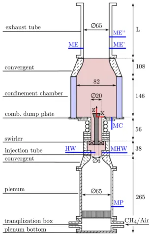
The investigated test rig is a confined premixed swirl combustor sketched in Fig. 1 and located at EM2C laboratory. The shaded pink area indicates the domain resolved by the LES. Additionally, the microphone locations (MP, MC, ME, ME’, ME”), the position of the hot-wire probe (HW), and the associated microphone (MHW) are shown.
A methane/air mixture is well premixed before it is injected in a tranquilization box, upstream of the plenum. The flow is then laminarized by a perforated plate followed by a honeycomb structure. It then passes through a first convergent (contraction ratio: 8.73) that generates a top-hat velocity profile at the inlet of the LES domain. Up to this position, the upstream parts including the plenum and the contraction have an acoustic equivalent length of 265 mm. A hot-wire probe is used to measure the velocity at the outlet of the convergent, where the diameter is 22 mm. The flow in this section is laminar with a top-hat axial velocity profile. After being pushed through a radial swirler, the fuel/air mixture enters the combustion chamber, which has a square cross section of 82 mm. The resulting turbulent, swirled-stabilized flame is V-shaped, anchored at a cylindrical bluff body that is topped by a cone. The combustion products are exhausted through a water-cooled convergent (contraction ratio: 2.03) with a square-to-round cross section, and an exhaust tube of variable length can be added optionally. The numerical LES domain, highlighted in red in Fig. 1, ends at the outlet of the exhaust convergent.
Fig. 1 Sketch of the EM2C turbulent swirl combustor for configuration B. Dimensions are given in millimeters.
A. Operating Conditions
Experiments are all presented for the same flow operating condition. A perfectly premixed methane/air mixture with an equivalence ratio of ϕ ! 0.82 and a thermal power of Pth! 5.5 kW is considered. In the
injection tube of diameter D ! 22 mm, the resulting bulk flow velocity is ub! 5.4 m∕s, yielding a Reynolds number of
approximately Re ! ubD∕ν ≃ 7000. Note that the flow remains
laminar in this section. Relative fluctuations of the velocity are less than 2% in the boundary layer and much lower within the core flow. The flow temperature in this section is equal to 300 K. The mean combustor exit velocity and Mach Number are ue! 2.8 m∕s and Ma ! 0.0043,
respectively. The thermoacoustic state of the combustor is modified by varying the exhaust tube length shown in Fig. 1. Three configurations are investigated and are designated by A, B, and C in the remainder of this study.
Without any exhaust tube (configuration A), the system is stable, and no distinct tone emerges from the pressure spectrum. The flame features in this case turbulent fluctuations without any detectable low-frequency self-sustained coherent motion.
Adding an exhaust tube of L ! 220 mm length on top of the exhaust convergent provokes a mild thermoacoustic instability with intermittent bursts and synchronized pressure oscillations at a frequency f ! 205 Hz (configuration B). The temperature of the gases in the exhaust tube is on average approximately T ! 1080 K. If the exhaust tube length is further increased to L ! 440 mm, the instability grows in amplitude and reaches a stable limit cycle with a fixed oscillation amplitude p0! 840 Pa in the combustion chamber
and an oscillation frequency equal to f ! 185 Hz (configuration C). In this case, the average temperature of the gases within the exhaust tube drops to approximately T ! 1000 K due to the larger heat transfer to the surrounding. A summary of the three configurations investigated is given in Table 1.
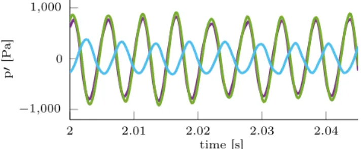
The instability at f ! 185 Hz is coupled to the 3/4 wave mode of the system. Figure 2 shows that the signal recorded by the microphone located in the plenum (MP, blue) is almost out of phase with respect to the signals measured by the microphones located in the confinement chamber (MC, green) and in the exhaust tube (ME, purple). Simulations carried out with a low-order thermoacoustic model of the combustor yields the same frequency and structure of the acoustic field.
B. Diagnostics
The thermoacoustic state of the combustor is characterized by the hot-wire probe HW and the microphone MHW placed in front of the hot wire, as sketched in the Fig. 1. The hot wire measures the velocity signal in the tube of 22 mm diameter before the swirler, where the flow is laminar with a top-hat velocity profile. A microphone MP is flush-mounted, before the convergent. A second microphone MC is mounted on a water-cooled wave guide that is itself connected to the backplate of the combustion chamber. Three additional microphones, which are also mounted on water-cooled wave guides, can be inserted on the exhaust tube to measure the combustor outlet reflection coefficient Rout using the three-microphone method [35]. All the
microphones are connected to preamplifiers (Brüel & Kjaer Type 4938-A-011) and then connected to a conditioning amplifier (Brüel & Kjaer Type 2690). All microphones are first calibrated with a known sound source (94 dB, 1000 Hz).
All signals are sampled at a frequency fs! 8192 Hz and recorded
for a duration of 4 s. This corresponds to around 1000 natural instability cycles for configuration C, of which a few are illustrated in Fig. 2.
Optical access in the confinement chamber is granted through the use of quartz walls, which are transparent for both the visible and
close ultraviolet wavelengths. OH"images of the average turbulent
flame structure and phase-conditioned images of the flame submitted to external acoustic forcing are recorded with an intensified charge-coupled device (ICCD) camera mounted with an interferometric filter centered on 310 nm with a 10 nm bandwidth. Abel deconvolutions are then performed on these images. Laser Doppler velocimetry is also used to analyze the flow at the swirling injector outlet in the absence of combustion. The three velocity components (axial, radial, and circumferential) velocities are measured by seeding the flow with small oil droplets of 2 μm in diameter. Velocity measurements are made 3 mm above the combustion chamber backplate.
C. Acoustic Boundary Conditions
Reflection of acoustic waves at the upstream and downstream terminations of the combustor needs to be considered to determine the sound pressure level (SPL) and the spectral content of the acoustic pressure field. At the bottom of the plenum, the test rig is terminated by a metallic thick rigid wall. This boundary is accordingly assumed to be fully reflective without any phase shift and the reflection coefficient is Rin! 1. The same plenum system with the same
components up to the injection tube before the hot-wire probe (HW) was already used in previous analysis of self-sustained combustion instabilities [36–38]. In these studies, it was also assumed that the bottom of the burner was a perfectly reflecting rigid plate and that the grid and honeycomb structure were transparent to sound waves. The excellent match in these references between model predictions and measurements for the different acoustic pressure and velocity signals strongly suggests that these assumptions are correct.
On the downstream side, the combustor exhaust is open to the atmosphere, and a fraction of the sound is radiated out of the combustor. The reflection coefficient Routat the downstream end is
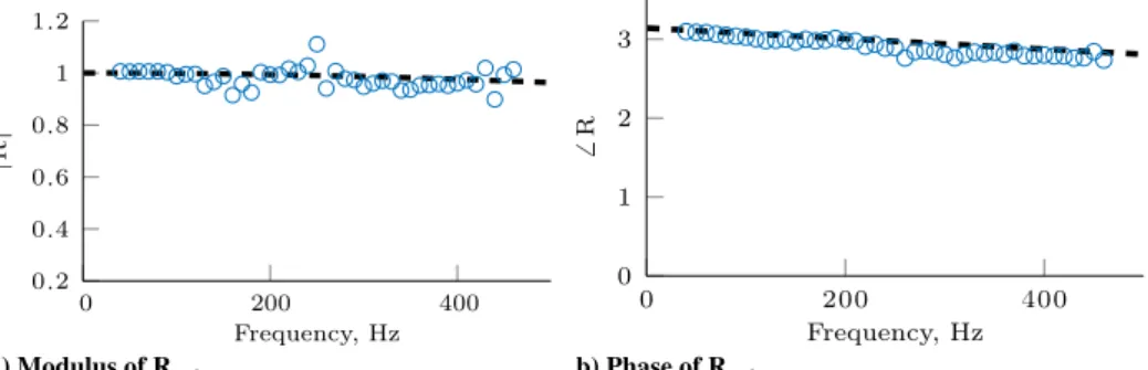
determined with three microphones mounted on water-cooled wave guides that are introduced on the exhaust tube shown in Fig. 1. The three-microphone method along with coherence functions and the switching method from Chung and Blaser [35] are used to determine Routbetween 20 and 500 Hz. These measurements shown in Fig. 3 are
carried out for the combustor operating at the nominal condition ϕ ! 0.82 and ub! 5.4 m∕s. It is found that reflection is well
reproduced by the Levine and Schwinger [39] model for an open-ended unflanged pipe.
III. Numerical Setup
The LES code AVBP [40] from CERFACS is used to assess the spectral sound distribution of the given setup. The fully compressible Navier–Stokes equations are solved on an unstructured grid [41,42]
Table 1 Summary of configurations studied
Configuration Exhaust tube length, mm Thermoacoustic state Frequency, Hz Amplitude Color
A 0 Stable — — — — Orange
B 220 Intermittent instability 205 u0∕ !u ! 0.2 Yellow
C 440 Instability at limit cycle 185 u0∕ !u ! 0.7 Green
Fig. 2 Pressure measurements at limit cycle of the instability at f! 185 Hz in configuration C. Plenum microphone (MP, blue), combustion chamber microphone (MC, green), and exhaust tube microphone (ME, purple).
by using the Lax–Wendroff scheme, which is of second-order accuracy in space and time. To reduce the computational effort, the LES domain is limited to the region downstream of the plenum contraction and upstream of the exhaust tube; see Fig. 1.
The unstructured grid consists of approximately 19 million tetrahedral cells with a maximum cell size of 0.6 mm in the flame region and 0.8 mm in the burner flow region, which consists of the swirler and the injection tube. The geometrical details of the swirler are fully modeled. The six radial swirler vanes, which have a diameter of 6 mm, are resolved by approximately 18 cells in the diameter that are refined toward the walls. In total, the swirler part is resolved by about 4 million cells.
Mesh independence of the results has been affirmed by testing one coarser and one finer mesh, compared to the reference mesh denoted as Mref. The different mesh resolutions result from a local refinement
in the flame region and the upstream flow region. The finer mesh M3 has a maximum cell size of 0.4 mm in the flame region and 0.6 mm in the upstream flow region, respectively, yielding a total cell number of approximately 34 million cells. For the coarser configuration M1, the mesh resolution was decreased in the flame region and the upstream flow region to 0.8 and 1.0 mm, respectively. This numerical configuration has a total cell number of approximately 11 million cells. The mesh resolution of the downstream flow region is kept constant with a cell size of 1.4 mm for two reasons.
1) The upstream flow region is of more relevance for the incoming flowfield of the flame and thus for the flame characteristics.
2) Less complex flow dynamics is expected in the downstream region due to the simpler geometry and the elevated viscosity in the burned gas region.
Table 2 summarizes the given values of the three meshes. Results of the velocity profiles at the combustion chamber inlet (nonreacting flow) as well as noise spectra (reacting flow) were compared for the three different meshes. Whereas the mean velocity profiles in axial, radial, and circumferential directions are almost identical for all three meshes, the fluctuating components deviate slightly for the coarsest mesh M1 compared to Mrefand M3. For the
reactive case, however, the resulting pressure spectra agree fairly well for all three meshes, even for the coarsest one. It is thus concluded that the results obtained for Mrefare mesh independent.
Subgrid stresses are handled by the wall adapting linear eddy (WALE) model [43], whereas interactions between the turbulent flowfield and the flame are described via the dynamically thickened flame model [44], resolving the laminar flame thickness within seven cells. The reduced two-step BFER scheme [45] is used to reproduce the chemistry of the premixed methane/air flame.
All parts upstream of the combustion chamber are assumed to be adiabatic. For the bluff body tip, a temperature of 1000 K is applied,
which is in agreement to measured values. For the combustion chamber walls, which are made out of quartz glass, a heat loss boundary condition is used. For that, the experimentally measured temperature at the outside of the quartz wall is imposed at the LES boundaries as a reference temperature and an according thermal resistance is defined. This allows the wall temperature in LES to have a spatially nonuniform temperature distribution and to adapt to the internal temperature field. The metallic combustor dump plate is assumed to have an isothermal temperature of 823 K. With these imposed wall temperatures and the respective heat losses, the exhaust gas temperature at the LES domain outlet is in good accordance with the measured mean exhaust gas temperature of configuration A of approximately 1150 K. Reproducing the temperatures and thus the speed of sound accurately in LES is of importance to correctly predict the frequencies of the thermoacoustically unstable modes and the resulting sound pressure spectra in general.
To correctly model the acoustic transmission and reflection of the up- and downstream components of the test rig that are not included in the numerical domain, the LES domain is coupled to characteristics-based state-space boundary conditions (CBSBCs) [46], which are described later in this section.
A. Extracting Acoustic Pressure Fluctuations
It has been proposed to combine incompressible LES with a source model based on the spatiotemporal variations of heat release fluctuations to predict combustion noise [47–49]. Alternatively, a fully compressible formulation of the Navier–Stokes equations allows to assess combustion noise directly and without the need of a source model. However, the pressure signal in a compressible LES is a superposition of the acoustic and hydrodynamic pressure fluctuations, which may make the separation of the two contributions challenging. Turbulent and acoustic fluctuations cover the same range of amplitudes and frequencies or are at least in the same order of magnitude. In the present study, the method of characteristics-based filtering (CBF) [50] is used to extract the acoustic pressure fluctuations from the LES pressure field. This method exploits the difference in propagation speed between turbulent and acoustic fluctuations and allows to identify acoustic waves in turbulent compressible flows.
B. Modeling of Acoustic Boundaries
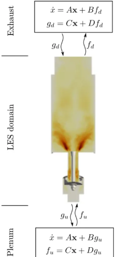
As already mentioned, correct acoustic modeling at boundaries of the numerical domain is crucial for predicting the sound pressure field inside the system as well as its thermoacoustic stability. Acoustic reflections at the boundaries may cause, for example, peaks in the sound pressure spectrum due to resonant amplification of acoustic eigenmodes or may couple with the flame dynamics to provoke a thermoacoustic instability. The acoustic characteristics of all components upstream and downstream of the numerical domain that are present in the test rig but are not resolved directly by LES and need to be modeled in an appropriate manner (see Fig. 4). This is achieved in the present study by using the characteristics-based state-space boundary conditions (CBSBCs) proposed by Jaensch et al. [46], which are a variant of time-domain impedance boundary conditions (TDIBC) [32,51–53].
a) Modulus of Rout b) Phase of Rout
Fig. 3 Comparison between measured reflection coefficient (circles) and model of Levine and Schwinger [39] for an open-ended unflanged pipe (dashed line).
Table 2 Summary of tested mesh resolutions
Mesh Burner region cell size,mm Flame region cell size,mm Total number ofcells M1 1 0.8 11.06 million Mref 0.8 0.6 19.08 million
In the simplest case, CBSBCs may be regarded as a fully nonreflective extension of the well known Navier–Stokes character-istic boundary conditions (NSCBCs) [54]. Like the NSCBCs, the CBSBCs avoid a drift of the mean flow variables. But whereas the NSCBCs yield a reflection coefficient of a first-order low-pass filter [55,56], the CBSBCs make use of plane wave masking [56] yielding a fully nonreflective behavior also at low frequencies. This behavior is achieved by an extension of the linear relaxation term of the NSCBCs that explicitly eliminates outgoing wave contributions from the linear relaxation term [56]. To identify accurately the outgoing wave contributions from the turbulent compressible flowfield, the CBF method is again applied.
In the present context, the main benefit of the CBSBCs is that they allow also to impose an ingoing wave, which effectively emulates a time-domain impedance with complete control over the phase and magnitude of the reflection coefficient. This is not feasible with the standard NSCBC formulation. This flexible and individual control of magnitude and phase allows to set complex reflection coefficients to the numerical domain. An exact description of the reflection conditions at the LES domain boundaries is achieved by imposing the measured impedances.
Because of the impact of the CBSBCs on the resulting sound pressure spectra, the coupling of the LES to the state-space model of the acoustic subsystem is explained in more detail. This is exemplarily done for the inlet boundary condition that describes the acoustic propagation within the plenum tube and the fully reflective plenum bottom. First, the upstream traveling characteristic wave
gu! 1 2 !p0 a !ρ !c− ua0 " u (1)
which is leaving the LES domain, is extracted by the CBF method. Herein, pa0 and ua0 represent the acoustic pressure and velocity
fluctuation, respectively, whereas !ρ and !c refer to the mean values of density and speed of sound. The CBF filtering allows a proper separation between acoustic and turbulent fluctuations by exploiting their different propagation speeds. Whereas the acoustic perturbations propagate with the speed of sound, turbulent fluctuations are transported with the convective velocity.
In a next step, the extracted characteristic wave guserves as an
input for the state-space model, which describes the acoustic processes downstream of the LES domain:
_
x ! Ax # Bgu (2a)
fu! Cx # Dgu (2b)
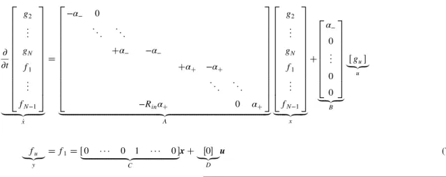
Herein, x denotes the state-vector of the boundary model. The model itself depends on the system matrices A, B, C, and D, which describe the acoustic properties of the state-space model. As demonstrated by Jaensch et al. [46], there are different approaches to determine the system matrices A, B, C, and D (e.g., from a set of partial differential equations, from a polynomial fit of measured reflection conditions at discrete frequencies, or even from an acoustic network model).
To help the reader to develop a better physical understanding of the state-space model in Eq. (2), the state-space model used for the inlet boundary condition is constructed in the following from a set of partial differential equations. The linearized Euler equations describe the plane wave acoustics within the plenum and read as
∂f ∂t # $u # !c%! ∂f ∂x !0 (3a) ∂g ∂t # $u!− !c% ∂g ∂x !0 (3b) with !u denoting the mean convective velocity within the plenum. Following the notation introduced in Fig. 5, the partial differential equation system is closed by the boundary conditions
g$x ! 0; t% ! g1! gu (4a)
f$x ! L; t% ! fN! Rin⋅ g$x ! L; t% (4b)
The boundary condition at x ! 0 provides the characteristic wave gu, which is extracted from the LES, as input to the boundary
state-space model. At x ! L, the reflected wave fNis described in terms of
the imposed reflection coefficient Rin. After applying a spatial
discretization of the plenum (e.g., a linear upwind finite difference scheme), Eqs. (3a) and (3b) yield
∂fi ∂t !−$ !u # !c% fi#1− fi Δx for i! 1; : : : ; N − 1 (5a) ∂gi ∂t !−$ !u − !c% gi− gi−1 Δx for i! 2; : : : ; N (5b) Combined with the boundary conditions of Eqs. (4a) and (4b), it follows for g2and fN−1
∂g2 ∂t !−$ !u − !c% g2− gd Δx (6a) ∂fN−1 ∂t !−$ !u # !c% Rin⋅ gN− fN−1 Δx (6b)
Fig. 4 LES domain coupled to CBSBCs via the characteristic waves f and g. Impedances of plenum and exhaust tube are modeled by CBSBCs.
From Eqs. (4–6), the state-space model can now be constructed as ∂ ∂t 2 6 6 6 6 6 6 6 6 6 6 6 6 6 4 g2 .. . gN f1 .. . fN−1 3 7 7 7 7 7 7 7 7 7 7 7 7 7 5 |######{z######} _ x ! 2 6 6 6 6 6 6 6 6 6 6 6 6 6 4 −α− 0 . . . . . . #α− −α− #α# −α# . . . . . . −Rinα# 0 α# 3 7 7 7 7 7 7 7 7 7 7 7 7 7 5 |####################################################{z####################################################} A 2 6 6 6 6 6 6 6 6 6 6 6 6 6 4 g2 .. . gN f1 .. . fN−1 3 7 7 7 7 7 7 7 7 7 7 7 7 7 5 |####{z####} x # 2 6 6 6 6 6 6 6 6 4 α− 0 .. . 0 0 3 7 7 7 7 7 7 7 7 5 |#{z#} B & gu' |{z} u fu |{z} y ! f1! & 0 · · · 0 1 · · · 0 ' |#####################{z#####################} C x # &0'|{z} D u (7)
where α#! $ !u # !c%∕Δx, and α−! $ !u − !c%∕Δx. The interpretation of the constructed state-space model is the following. The state vector x contains the values of f and g at the discrete locations. The state matrix A is mainly determined by the discretization scheme and describes the wave propagation along the characteristics on its main diagonals. However, the off-diagonal element relates the values fN−1
and gNin terms of the prescribed reflection coefficient Rin. The vector
B denotes the input vector and describes the influence of the input quantity guon the system. The output vector C defines which values
of the state vector x serve as outputs and are consequently fed back into the LES. In the present case, only the value corresponding to f1! fuis nonzero, meaning that, at the LES inlet, an acoustic wave
is imposed with fu! 1 2 !p0 a ! ρ !c #ua0 " u (8)
Here, fuis the time-lagged reflection of the acoustic wave gu. The
time lag depends on the length of the plenum L and the speed of sound c. Because no additional external excitation is imposed at the LES inlet, the feedthrough vector D is a null vector.
The coupling between LES and CBSBC at the outlet of the numerical domain is established in an analogous manner. However, the respective state-space model is constructed from a polynomial function, representing the Levine–Schwinger conditions for an open unflanged pipe [39]. For the details of this alternative approach and further information on the CBSBC formulation, the reader is referred to the publication of Jaensch et al. [46]. Note that the coupling of a compressible LES to CBSBC was already used successfully by Jaensch et al. [57] and Tudisco et al. [58].
C. Acoustic Boundary Conditions of the Numerical Domain The three configurations A, B, and C feature different reflection coefficients at the boundaries of the numerical domain. All three configurations share the same acoustic impedance at the numerical
domain inlet, which is characterized by the reflection coefficient Rin
shown in Fig. 6. This boundary condition models the acoustic impedance of the plenum terminated by a rigid wall. According to the hard wall at the upstream end of the plenum (see Sec. II.C), the absolute value of the reflection coefficient remains constant and equal to unity across all frequencies jRinj ! 1. The plenum itself
introduces a frequency-dependent phase lag that only depends on the plenum length and the speed of sound within the plenum. For the given plenum, the acoustic equivalent length of l ! 265 mm, and the speed of sound of c ! 340 m∕s, a phase lag as shown in Fig. 6b results.
The outlet reflection coefficient Rout, however, changes between
the three configurations studied and has a major impact upon the resulting sound pressure spectra in the combustion chamber. Because all three configurations are open-ended, the magnitude of Rout is thus the same for all three configurations. The Levine–
Schwinger condition [39] for an open-ended unflanged pipe is applied as shown in Fig. 7a. Even though experimental data are only available up to 500 Hz, the analytical expression allows a reliable definition of the reflection coefficient in the LES up to higher frequencies. But for a better readability, only the frequency range [0–1000 Hz] is depicted in Fig. 7. The reflection coefficient Routat
the numerical domain outlet is fully reflective in the low-frequency limit and introduces a slight decrease of the reflection magnitude with increasing frequencies. The decay rate of∠Routis a function of
the exhaust tube length, diameter, and speed of sound. For configuration A, the Levine–Schwinger condition can directly be used for Rout, as shown by Fig. 7b (orange). However, for
configurations B and C, an additional phase lag has to be taken into account due to the additional length of the exhaust tube. This phase lag increases linearly with the exhaust tube length. For both configurations, a mean speed of sound of c ! 634 m∕s was assumed, corresponding to a mean exhaust gas temperature of Tout! 1000 K. Figure 7b also shows the phase of the reflection
coefficient for configurations B (orange) and C (green).
a) Modulus of Rin b) Phase of Rin
IV. Results
An overview of the LES carried out for the different cases explored is given in Table 1 together with the dynamic state of the system observed in the experiments. Note that the plenum and exhaust tubes could also be modeled directly by the LES, similar to the setup of Franzelli et al. [59], but this would significantly increase the numerical domain size and thus the computational effort. Moreover, a remeshing would be necessary for every configuration investigated. The chosen coupling of LES and CBSBC allows to analyze changes in acoustic impedance at the numerical domain boundaries by a simple reformulation of the state-space model. Practically, this means that the LES numerical domain remains the same for all three configurations, and the resulting instability only arises due to the reformulation of the boundary state-space model at the numerical domain outlet.
A. Velocity Profiles
The velocities measured by LDV in the experiments are first compared to the numerical results under cold flow operation for a bulk velocity of ub! 5.4 m∕s at the numerical domain inlet. In LES,
the averaging time amounts to 240 ms and corresponds thus to approximately 16 flow trough times. The velocity profiles are compared 3 mm above the combustion chamber dump plate.
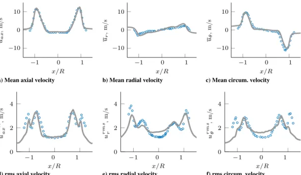
Figures 8a–8c show an excellent agreement for all three velocity components between measurements and LES computations. In this figure, the radial distance x to the burner axis is normalized by the injector outlet radius R ! 10 mm. The radial location of the velocity
peaks and their associated amplitudes are correctly predicted by the numerical results.
The measured rms values are slightly less well reproduced by the simulations. The rms values of the axial velocity are still in fairly in good agreement in Fig. 8d between experiments and LES, whereas the rms velocity profiles of the radial and circumferential velocity profile show some discrepancy in Figs. 8e and 8f. Even though the respective total values are in the same range of magnitude, the values downstream the bluff body close to x∕R ! 0 and in the outer shear layer x∕R ( 1 differ slightly.
One possible reason might be that the relatively short time in the LES over which averages were made is not long enough to converge toward the correct average values that were found to be statistically independent of the number of samples in the experiments. The LDV measurements are also averaged over the collection volume probed by the laser beams. This might also introduce a small bias in the measurements, especially in the regions of high shear due to the large gradients. The overall comparison between mean and rms velocity profiles for the three velocity components, however, yields satisfying agreement for the cold flow condition explored.
B. Shape of Mean Reaction Zone
Because velocity measurements are only available for cold flow conditions, as a first step, the comparison with simulations is further investigated in reacting conditions by examining the mean reaction zone shape.
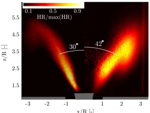
The mean shape taken by the flame in configuration A, when the combustor is stable, is shown in Fig. 9 in the midlongitudinal plane of a) Modulus of Rout b) Phase of Rout
Fig. 7 Complex outlet reflection coefficient used in the numerical model. Left: modulus for configurations A, B, and C. Right: phase for configuration A (orange), B (yellow), and C (green).
a) Mean axial velocity b) Mean radial velocity c) Mean circum. velocity
d) rms axial velocity e) rms radial velocity f) rms circum. velocity
Fig. 8 Cold flow velocity fields (axial, radial, circumferential) measured by LDV (circles) and LES results (solid line). Top: mean values. Bottom: rms values.
the combustion chamber. The combustor dump plate and the central bluff body are sketched in gray. The flow is directed from bottom to top. On the left-hand side, the distribution of the volumetric heat release rate calculated by LES is depicted. Results are normalized by the maximum value found in the simulation and averaged over data accumulated over 120 ms. The right-hand side of Fig. 9 shows the Abel transform of the OH"experimental signal recorded over 100 frames with an exposure
time of 20 ms for each snapshot. Five frames were taken each second, which amounts to a total integration time of 20 s. At this point, it is emphasized that the measured mean reaction zone shape and the one resulting from LES can only be compared to a certain extent. The measured Abel transformed images depict the OH"
chemilumines-cence distribution, whereas LES results represent the mean reaction zone in terms of heat release rate. The global two-step reaction scheme of the LES cannot be used to infer the OH"distribution.
Figure 9 indicates that the simulated mean reaction zone shape is in reasonable agreement with that observed in experiments. Even though the flame angle at the injector outlet differs by about 12 deg, the positions of the flame leading edge and the flame height are fairly well reproduced by the LES. The flame length is an essential feature that governs the cutoff frequency of the flame transfer function [60] and has also be shown to be an important parameter that governs the peak frequency of the broadband combustion noise radiated by unconfined flames [10]. A reasonable reproduction of the flame length is thus compulsory to reproduce the sound pressure spectra.
In configuration C, the system is unstable, and the oscillation reaches a limit cycle with a frequency of 185 Hz. This is also what is observed in the numerical simulation of this configuration. A comparison is made of phase-averaged flame images in Fig. 10. These pictures shed additional light on the flame dynamics and the flame motion during one oscillation cycle.
The images recorded in the experiments, on the right-hand side in Fig. 10, show OH"phase-averaged and Abel transformed images. In
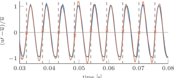
this case, each frame corresponds to an exposure time of 40 μs, and results are averaged over 100 frames. These images are synchronized with respect to the velocity signal measured by the hot-wire probe HW in the injection tube, shown in Fig. 11. The mean reaction zone shapes from LES, shown on the left-hand side in Fig. 10, are represented by a heat release rate isocontour averaged over 20 frames at the same phase angles in the oscillation cycle as in the experiments. The time covered by the 20 LES frames adds up to approximately 110 ms. Every LES flowfield is sliced along the x axis, the y axis, and the two bisectors, yielding in total eight flame halves to average across per frame. In the LES, the sampling frequency is set constant and equal to a sixth of the oscillation frequency of the instability. Because of small cycle-to-cycle variations caused by the acoustic velocity fluctuations induced by the flame, the phase angle of the respective snapshots (×) is slightly varying in respect to the inlet velocity signal. The time instants at which the ICCD camera is triggered in the experiment is marked by the dashed vertical lines and
a) Phase angles 0°-120°
b) Phase angles 180°-300°
Fig. 10 Phase-averaged flame images over one oscillation at limit cycle for configuration C. Left: LES. Right: experiment. The coordinates are normalized with the injection tube radius R ! 10 mm.
Fig. 9 Mean reaction zone shape for stable configuration A. Left: LES results temporally averaged over 120 ms. Right: Abel deconvolution of the OH"signal averaged over 100 frames.
is controlled by the phase angle of the velocity signal in the injection tube.
The general flame motion during the oscillation cycle is satisfyingly described by the compressible LES in Fig. 10. The position of the largest structures of the flame and the respective flame length are fairly well reproduced by the LES at each phase of the oscillation cycle. Flame length increase per phase increase is captured by the simulation as well as the radial flame extension observed in the experiments. Despite the limitations of this qualitative comparison, such as the slightly varying phase angle of the respective snapshots or the comparison between OH"
chemiluminescence and heat release rate, it can be concluded that the compressible LES is capable of describing the main important features of the flame motion during a limit-cycle oscillation. C. Sound Pressure Spectra
The acoustic pressure time series recorded in the experiments are statistically averaged by the use of Welch’s power spectral estimate because a direct use of the fast Fourier transform has no meaning for noisy signals over a finite duration of time. Thirty-two Blackman– Harris windows are used with an overlap of 50% over the 4-s-long experimental time series. The numerical time series are postprocessed with only three Blackman–Harris windows because they have a length of only 360 ms. The sound pressure level (SPL) is defined here as
SPL! 20 × log10 !p0 rms pref " (9)
with a reference pressure pref! 2. × 10−5Pa. Sound pressure
signatures are compared between experiments and simulations for the microphone MC set in the combustion chamber (see Fig. 1).
A first calculation is made by imposing perfectly nonreflective boundary conditions at the inlet and outlet of the numerical domain. This situation mimics an open flame radiating noise as long as the acoustic wavelength is significantly larger than the characteristic transverse dimensions of the combustor. The power spectral density of the SPL signal is here compared to the theoretical spectrum from Clavin and Siggia [14]. Their analytical scaling law is based on the assumption of a Kolmogorov turbulence spectrum and predicts that the power spectral density of the noise radiated by an unconfined turbulent flame features a decay proportional to f−2.5, where f is the
frequency.
Figure 12 shows the computed sound pressure spectrum for nonreflective boundary conditions at the inlet and outlet (gray). By determining from LES the bulk flow velocity at the combustion chamber inlet uave and the distance between the maximum heat
release and the burner exit plane Lf, the Strouhal number scaling
proposed by Winkler et al. [13] can be applied:
St !fpeaku Lf
ave
≃ 1 (10)
From LES, the values of uave! 7.1 m∕s and Lf≃ 0.028 m are
found, resulting in an estimated peak frequency of fpeak≃ 250 Hz.
The spectral decay rate above the peak frequency is well reproduced by the decaying scaling law of Clavin and Siggia [14] (dashed line). One may conclude that all relevant mechanisms responsible for the generation and propagation of acoustic waves in the turbulent combustion process are described qualitatively correct by the LES.
Additionally, the sound pressure spectrum of the nonreflective case is overlaid with the sound pressure spectrum that results from applying the fully reflective boundary conditions of configuration A (orange). Even though the spectrum for configuration A is discussed in more detail in the next section, two aspects are already worth emphasizing at this point. First, compared to the reflecting conditions of configuration A, no distinct peaks emerge from the pressure spectrum if nonreflective boundary conditions are applied. Second, the general spectral shape of the case with nonreflecting boundary conditions is preserved in the spectrum of configuration A. Especially the spectral rolloff at higher frequencies is also visible for configuration A, although distinct peaks resulting from cavity resonances are observable.
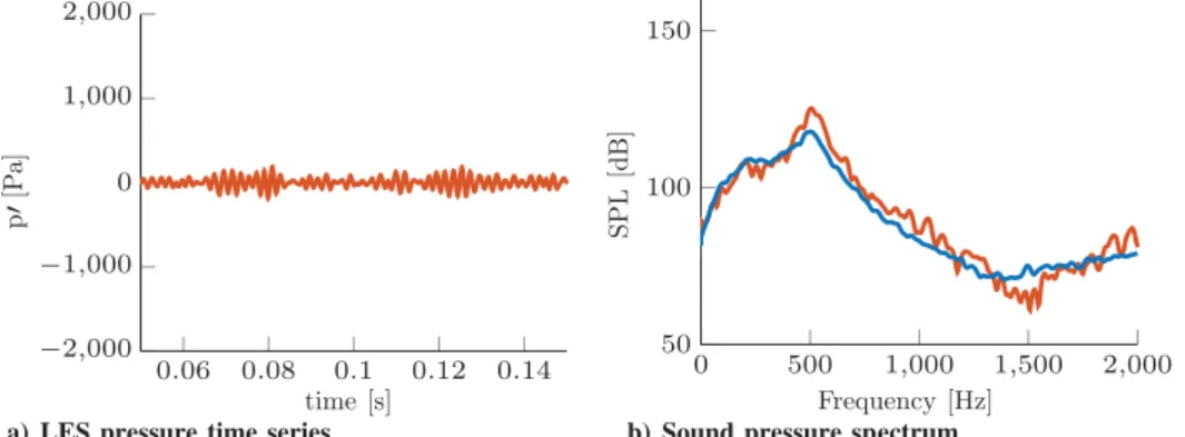
Figure 13 shows on the left 100 ms of the computed pressure time series (orange) for configuration A when the system is stable with respect to thermoacoustic instabilities but features reflection at its inlet and outlet. The exhibited pressure fluctuations of the time series remain small. On the right-hand side, the measured (green) and computed (orange) sound pressure power spectral distributions are depicted. One observes a remarkable agreement between the measured and simulated values. In the low-frequency limit, the slope of the pressure spectral distribution and its level are in overall good agreement. The level at the peak frequency at around 500 Hz is slightly overpredicted by 7 dB in the LES. This slight difference between measurements and the LES is mainly attributed to the differences in the mean reaction zone shape, observed in Fig. 9. This is believed to be the main origin of discrepancies in the low-frequency region and at the peak frequency. The subsequent measured decay of the SPL is well reproduced by LES coupled to CBSBCs. The slight difference between measurements and the LES prediction in the region of the local minimum around 1500 Hz can be mainly attributed to the uncertainties in the thermal boundaries. Inaccuracies in the temperature field yield to a shift of frequencies in the LES, especially in the higher-frequency regions.
According to theory and the spectral distribution of the nonreflective configuration shown in Fig. 12, the combustion noise source in Fig. 13 is mainly active in the midfrequency region up to 300 Hz and rolls off to higher frequencies. However, the spectral sound pressure distribution is no longer completely flat over the whole frequency range. The appearance of the peak at 500 Hz with an amplitude of approximately 120 dB may be seen as the combustor resonance. The broadband noise emitted by the flame goes in resonance with the system cavities. Depending on the cavity Fig. 12 Spectral sound pressure distribution from LES with nonreflective boundary conditions (gray), with partially reflecting conditions of configuration A (orange) and prediction of spectral decay by [14] (dashed line).
Fig. 11 Velocity signals used for the synchronization: measured at MHW (blue), LES inlet velocity (orange), triggering of ICCD camera (dashed line), snapshot in the LES (×).
geometry, certain frequencies are damped, and others are amplified, resulting in the formation of peaks in the spectral sound pressure distribution. By using a linear acoustic network model of the combustor [61], the resonant peak in the sound pressure spectrum of configuration A can be identified as the 3∕4λ wave mode of the system that is resonating. Nonetheless, the combustion remains stable, and the overall SPL magnitude remains at a moderate level.
Figure 14 shows the results obtained for configuration B featuring an intermittent thermoacoustic instability at an oscillation of approximately 205 Hz. The computed time series shown in Fig. 14a demonstrates the intermittent behavior that manifests in the pressure signal. A distinct oscillating frequency is observable that grows in amplitude. At a certain amplitude level, the oscillation breaks down and starts to grow again. With respect to the time series shown in Fig. 13a, larger pressure fluctuations are reached. Compared to the pressure spectrum shown in Fig. 13b for the stable configuration A, an elevated SPL is reached in Fig. 14 with a peak amplitude of approximately 140 dB. The resulting SPL peak amplitude measured in the experiments is correctly reproduced by LES, with a difference of less than 5 dB. The rest of the spectral sound pressure distribution is also well reproduced by the simulation with a broad hump around 1000 Hz and a second smaller one at about 1750 Hz.
Using LES to simulate the spectral distribution of the sound pressure in presence of a thermoacoustic instability is a challenging task. The peak frequency and the peak amplitude significantly depend on the nonlinear coupling between acoustics and flame dynamics. In the respective sound pressure spectrum, this manifests by a peak at the frequency of the instability. The fully compressible LES strategy coupled with CBSBC is, however, capable of resolving directly both contributions and consequently also their nonlinear interaction. The main difference observed in configuration B is the spread of spectral energy around the peak frequency, which is much larger in the simulation than in the experiment. This might be due to the slight difference in the mean reaction zone shape already noticed in Fig. 9. But it is also worth recalling that regime B is unstable by
intermittence, meaning that the system does not reach a well defined limit cycle at a constant oscillation frequency and amplitude. The lock on of the instability frequency with the combustor resonant frequency is only achieved intermittently. This is a challenging configuration, in which subtle changes of the flow alter the thermoacoustic state of the system. Differences in turbulence might be the origin of the broader peak observed in the simulation.
The reader is reminded that this simulation is carried out by modifying only the reflection coefficient at the numerical domain outlet with the model shown in Fig. 7 (orange). This change is enough to reproduce the thermoacoustic instability in the LES with yet a reasonable match with experiments of the spectral content below 2000 Hz.
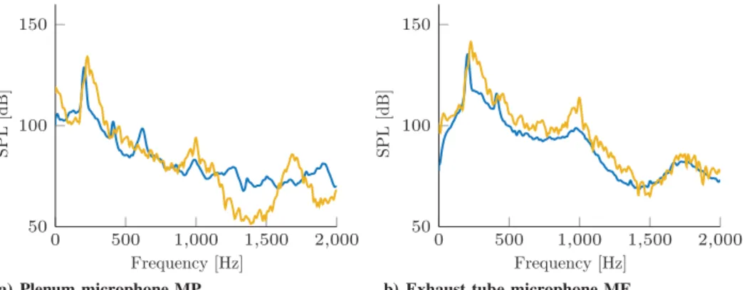
In addition to the pressure signal measured by microphone MC located in the combustion chamber, the signals measured by the microphones MP in the plenum and ME in the exhaust tube (see Fig. 1) are also compared to the computed data for configuration B. Note that the LES domain does not comprise the locations of MP and ME. The pressure signals needed for computing the respective sound pressure spectra cannot be extracted directly from the LES. Instead, the pressure time series are reconstructed from the state-space model used within the CBSBC. Therefore, the characteristic acoustic waves leaving the LES domain are stored during the computation. In an additional postprocessing step, these signals are used as input signals to simulate the boundary state-space model forward in time and thus compute the pressure signal at a given location. The resulting spectra are shown in Fig. 15. The sound pressure spectrum measured by microphone MP located in the plenum exhibits smaller pressure amplitudes over all frequencies compared to the signal measured by microphone MC in the combustion chamber. This is correctly predicted by the reconstructed numerical spectrum in Fig. 15a, even though certain differences are observed for frequencies higher than 1000 Hz. The reconstruction of the signal in the exhaust tube at the microphone location ME is in very good agreement with the measured spectrum in Fig. 15b. The reconstructed peak amplitude
a) LES pressure time series b) Sound pressure spectrum
Fig. 13 LES pressure time series and sound pressure spectrum of the stable configuration A. SPL measurements (blue) and LES results (orange) for microphone MC.
a) LES pressure time series b) Sound pressure spectrum
Fig. 14 LES pressure time series and sound pressure spectrum of the intermittent unstable configuration B. SPL measurements (blue) and LES results (yellow) for microphone MC.
differs by about 4 dB from the measured one. The secondary bumps at around 1000 and 1600 Hz are well captured by the reconstructed spectrum. As already mentioned for the pressure spectra shown in Fig. 14, the main differences between the measured and reconstructed spectra in the plenum and exhaust tube are the width of the pressure peak of the thermoacoustic instability.
It is emphasized that the explained reconstruction procedure would not be applicable for TDIBC like they are used, for example, by Lourier et al. [32], in which the acoustic boundary impedances are modeled globally. Yet the used CBSBC describes duct sections within the state-space model as spatially discretized elements on which an advection equation is solved numerically. The according state variables may be assessed at every discretized element. Therefore, the CBSBC provides also spatial information of the state variables within the boundary model. However, the reconstructed pressure time series directly depend on the input time series (i.e., the extracted characteristic waves at the LES domain boundary). Errors made in the LES propagate directly into the reconstructed time series. Nevertheless, the overall good agreement between measured and reconstructed sound pressure spectrum proves that the CBSBC allows to reconstruct the main features of the measured signals even out of the LES numerical domain.
Last, the sound pressure spectrum obtained from LES (green) is compared to the measured one (blue) in configuration C at the limit cycle of the instability in Fig. 16. The thermoacoustic instability has a peak frequency of 185 Hz where the SPL reaches 150 dB in the combustion chamber. The LES now well reproduces not only the correct peak value of the pressure oscillation but also the same shape of the power spectral distribution around this frequency. The self-sustained oscillation reaches in this case a much larger oscillation amplitude of u0∕ !u ! 0.7 at the hot-wire location in the injection tube.
Compared to the intermittent configuration B, a well-defined limit cycle is reached in configuration C. In this case, reproducing turbulent fluctuations is of less importance for the determination of the exact thermoacoustic state around the instability frequency. This may explain why the shape of the spectral distribution is better
reproduced in configuration C compared to the intermittent state B. However, in the region above 500 Hz, a slight shift of the LES results to higher frequencies is observable. Again, this is probably due to the uncertainties regarding the temperatures in the exhaust tube region. If the mean gas temperature in the CBSCB model is overestimated, a shift to higher frequencies results.
Compared to the stable configuration A without exhaust tube (L ! 0) and a peak frequency around 500 Hz, the distinctively lower value of the peak frequency in configuration C is explained by the elongated cavity (L ! 440 mm) that shifts the acoustic modes to lower frequencies. As for configuration B, the instability in the LES is only provoked through a change of the outlet reflection condition of the numerical domain according to the model shown in Fig. 7 (green). Also for configuration C, in which the thermoacoustic instability is even more pronounced than in configuration B, the compressible LES coupled to CBSBC reproduces accurately the measured data for the sound pressure spectral distribution.
V. Conclusions
In the present study, the spectral sound pressure distribution of a confined lab-scale swirl combustor has been investigated by combining experiments and simulations. The flowfield and the mean reaction zone shape have been characterized as well as the acoustic fields for thermoacoustic stable, intermittently unstable, and unstable states of the test rig. The burner is operated with a methane/air mixture of constant flow injection conditions; the stability is only varied by changing the exhaust tube length. The turbulent flowfield, the flame, and the acoustics are resolved by performing fully compressible large-eddy simulation (LES) computations. It has been shown that the correct description of the complex acoustic boundary conditions from the test rig in the numerical approach is of crucial importance to correctly predict the resulting sound pressure spectrum and the sound level. The CBSBC formulation has proven itself to be very convenient for the description of the acoustic boundaries in the computational approach. They allow the correct modeling of the
a) Plenum microphone MP b) Exhaust tube microphone ME
Fig. 15 Sound pressure spectrum of the intermittent unstable configuration B in a) the plenum, and b) the exhaust tube. SPL measurements (blue) and CBSBC reconstruction (yellow).
a) LES pressure time series b) Sound pressure spectrum
Fig. 16 LES pressure time series and sound pressure spectrum at the limit cycle of the unstable configuration C. SPL measurements (blue) and LES results (green) for microphone MC.
different experimental configurations investigated without resolving all parts of the test rig within the LES numerical domain. Consequently, the thermoacoustically stable as well as the unstable combustion regimes could be well reproduced by a simple reformulation of the boundary inherent state-space model. The acoustic pressure fluctuations are extracted via a characteristics-based filter from the compressible LES. Accordingly, computed sound pressure spectra have been compared to the measured spectra. Excellent qualitative and quantitative agreement of resulting sound pressure spectra has been achieved for stable and unstable working conditions. Slight differences were identified for the intermittent unstable regime, probably due to difficulties in reproducing the same turbulent flow and reacting fields in the LES. But even in this case, the developed strategy could reproduce the main spectral features of the measured data with a fairly good fidelity. This holds not only for the combustion chamber that is comprised in the LES domain. Also the sound pressure spectra within the plenum and exhaust tube, which are located outside the numerical domain, could be reconstructed from the boundary state-space model.
Acknowledgments
The authors acknowledge financial support by the German Research Foundation, project PO 710/16-1, and by the Agence Nationale de la Recherche, NOISEDYN project (ANR-14-CE35-0025-01). This project also has received funding from the European Union’s Horizon 2020 Research and Innovation Programme under the Marie Sklodowska-Curie grant agreement number 643134. Moreover, the authors gratefully acknowledge the Gauss Centre for Supercomputing (GCS) for funding this project by providing computing time on the GCS Supercomputer SuperMUC at Leibniz Supercomputing Centre. The authors would also like to acknowledge Christian Kraus from Institut de Mécanique des Fluides de Toulouse for pointing out the incompatibility of the Wall Adapting Linear Eddy (WALE) model model and wall functions.
References
[1] Dowling, A. P., and Mahmoudi, Y., “Combustion Noise,” Proceedings of the Combustion Institute, Vol. 35, No. 1, 2015, pp. 65–100. doi:10.1016/j.proci.2014.08.016
[2] Burnley, V. S., and Culick, F. E., “Influence of Random Excitations on Acoustic Instabilities in Combustion Chambers,” AIAA Journal, Vol. 38, No. 8, 2000, pp. 1403–1410.
doi:10.2514/2.1116
[3] Strahle, W. C., “Combustion Noise,” Progress in Energy and Combustion Science, Vol. 4, No. 3, 1978, pp. 157–176.
doi:10.1016/0360-1285(78)90002-3
[4] Candel, S., Durox, D., Ducruix, S., Birbaud, A.-L., Noiray, N., and Schuller, T., “Flame Dynamics and Combustion Noise: Progress and Challenges,” International Journal of Aeroacoustics, Vol. 8, No. 1, 2009, pp. 1–56.
doi:10.1260/147547209786234984
[5] Ihme, M., “Combustion and Engine-Core Noise,” Annual Review of Fluid Mechanics, Vol. 49, Jan. 2017, pp. 277–310.
doi:10.1146/annurev-fluid-122414-034542
[6] Marble, F. E., and Candel, S. M., “Acoustic Disturbance from Gas Non-Uniformities Convected Through a Nozzle,” Journal of Sound and Vibration, Vol. 55, No. 2, 1977, pp. 225–243.
doi:10.1016/0022-460X(77)90596-X
[7] Schuller, T., Durox, D., and Candel, S., “Dynamics of and Noise Radiated by a Perturbed Impinging Premixed Jet Flame,” Combustion and Flame, Vol. 128, Nos. 1–2, 2002, pp. 88–110.
doi:10.1016/S0010-2180(01)00334-0
[8] Strahle, W. C., “On Combustion Generated Noise,” Journal of Fluid Mechanics, Vol. 49, No. 2, 1971, pp. 399–414.
doi:10.1017/S0022112071002167
[9] Ihme, M., Pitsch, H., and Bodony, D., “Radiation of Noise in Turbulent Non-Premixed Flames,” Proceedings of the Combustion Institute, Vol. 32, No. 1, 2009, pp. 1545–1553.
doi:10.1016/j.proci.2008.06.137
[10] Rajaram, R., and Lieuwen, T., “Acoustic Radiation from Turbulent Premixed Flames,” Journal of Fluid Mechanics, Vol. 637, Oct. 2009, pp. 357–385.
doi:10.1017/S0022112009990681
[11] Hirsch, C., Wäsle, J., Winkler, A., and Sattelmayer, T., “A Spectral Model for the Sound Pressure from Turbulent Premixed Combustion,” Proceedings of the Combustion Institute, Vol. 31, No. 1, 2007, pp. 1435–1441.
doi:10.1016/j.proci.2006.07.154
[12] Schlimpert, S., Koh, S., Pausch, K., Meinke, M., and Schröder, W., “Analysis of Combustion Noise of a Turbulent Premixed Slot Jet Flame,” Combustion and Flame, Vol. 175, Jan. 2017, pp. 292–306. doi:10.1016/j.combustflame.2016.08.001
[13] Winkler, A., Wäsle, J., Hirsch, C., and Sattelmayer, T., “Peak Frequency Scaling of Combustion Noise From Premixed Flames,” Proceedings of the 13th International Congress on Sound and Vibration, The International Inst. of Acoustics and Vibration (IIAV), Auburn, AL, 2006. [14] Clavin, P., and Siggia, E. D., “Turbulent Premixed Flames and Sound Generation,” Combustion Science and Technology, Vol. 78, Nos. 1–3, 1991, pp. 147–155.
doi:10.1080/00102209108951745
[15] Mahan, J. R., and Karchmer, A., “Combustion and Core Noise,” Noise Sources, Vol. 1, Aeroacoustics of Flight Vehicles: Theory and Practice, NASA, 1991, pp. 483–517.
[16] Bellucci, V., Schuermans, B., Nowak, D., Flohr, P., and Paschereit, C. O., “Thermoacoustic Modeling of a Gas Turbine Combustor Equipped with Acoustic Dampers,” Journal of Turbomachinery, Vol. 127, No. 2, 2005, pp. 372–379.
doi:10.1115/1.1791284
[17] Weyermann, F., Hirsch, C., and Sattelmayer, T., “Influence of Boundary Conditions on the Noise Emission of Turbulent Premixed Swirl Flames,” Combustion Noise, edited by J. Janicka, and A. Schwarz, Springer–Verlag, Berlin, 2009, pp. 161–188.
[18] Muthukrishnan, M., Strahle, W. C., and Neale, D. H., “Separation of Hydrodynamic, Entropy, and Combustion Noise in a Gas Turbine Combustor,” AIAA Journal, Vol. 16, No. 4, 1978, pp. 320–327. doi:10.2514/3.60895
[19] Habisreuther, P., Bender, C., Petsch, O., Büchner, H., and Bockhorn, H., “Prediction of Pressure Oscillations in a Premixed Swirl Combustor Flow and Comparison to Measurements,” Flow, Turbulence and Combustion, Vol. 77, Nos. 1–4, 2006, pp. 147–160.
doi:10.1007/s10494-006-9041-7
[20] Lamraoui, A., Richecoeur, F., Schuller, T., and Ducruix, S., “A Methodology for on the Fly Acoustic Characterization of the Feeding Line Impedances in a Turbulent Swirled Combustor,” Journal of Engineering for Gas Turbines and Power, Vol. 133, No. 1, 2011, Paper 011504. doi:10.1115/1.4001987
[21] Grimm, F., Ewert, R., Dierke, J., Reichling, G., Noll, B., and Aigner, M., “Efficient Combustion Noise Simulation of a Gas Turbine Model Combustor Based on Stochastic Sound Sources,” American Soc. of Mechanical Engineers Paper GT2015-42390, New York, 2015. doi:10.1115/GT2015-42390
[22] Zhang, F., Habisreuther, P., Bockhorn, H., Nawroth, H., and Paschereit, C. O., “On Prediction of Combustion Generated Noise with the Turbulent Heat Release Rate,” Acta Acustica United with Acustica, Vol. 99, No. 6, 2013, pp. 940–951.
doi:10.3813/AAA.918673
[23] Silva, C. F., Leyko, M., Nicoud, F., and Moreau, S., “Assessment of Combustion Noise in a Premixed Swirled Combustor via Large-Eddy Simulation,” Computers & Fluids, Vol. 78, April 2013, pp. 1–9. doi:10.1016/j.compfluid.2010.09.034
[24] Kings, N., Tao, W., Scouflaire, P., Richecoeur, F., and Ducruix, S., “Experimental and Numerical Investigation of Direct and Indirect Combustion Noise Contributions in a Lean Premixed Laboratory Swirled Combustor,” Proceedings of the ASME Turbo Expo 2016: Turbomachinery Technical Conference and Exposition, American Soc. of Mechanical Engineers Paper GT2016-57848, New York, 2016. doi:10.1115/GT2016-57848
[25] Lourier, J. M., Stöhr, M., Noll, B., Werner, S., and Fiolitakis, A., “Scale Adaptive Simulation of a Thermoacoustic Instability in a Partially Premixed Lean Swirl Combustor,” Combustion and Flame, Vol. 183, Sept. 2017, pp. 343–357.
doi:10.1016/j.combustflame.2017.02.024
[26] Flemming, F., Sadiki, A., and Janicka, J., “Investigation of Combustion Noise Using a LES/CAA Hybrid Approach,” Proceedings of the Combustion Institute, Vol. 31, No. 2, 2007, pp. 3189–3196.
doi:10.1016/j.proci.2006.07.060
[27] Bui, T., Schröder, W., and Meinke, M., “Numerical Analysis of the Acoustic Field of Reacting Flows via Acoustic Perturbation Equations,” Computers & Fluids, Vol. 37, No. 9, 2008, pp. 1157–1169.
doi:10.1016/j.compfluid.2007.10.014
[28] Hoeijmakers, M., Kornilov, V., Lopez Arteaga, I., de Goey, P., and Nijmeijer, H., “Intrinsic Instability of Flame-Acoustic Coupling,”