Any correspondence concerning this service should be sent to the repository administrator:
[email protected]
To link to this article : DOI:
10.1016/j.pepi.2016.05.017
URL :
http://dx.doi.org/10.1016/j.pepi.2016.05.017
This is an author-deposited version published in:
http://oatao.univ-toulouse.fr/
Eprints ID: 16158
O
pen
A
rchive
T
oulouse
A
rchive
O
uverte (
OATAO
)
OATAO is an open access repository that collects the work of Toulouse
researchers and makes it freely available over the web where possible.
To cite this version: Khan, Amir and van Driel, Martin and Böse, Maren
and Giardini, Domenico and Ceylan, Savas and Yan, Jun and Clinton,
John Francis and Euchner, Fabian and Lognonné, Philippe and Murdoch,
Naomi and Mimoun, David and Panning, Mark and Knapmeyer, Martin
and Banerdt, W. Bruce Single-station and single-event marsquake location
and inversion for structure using synthetic Martian waveforms. (2016)
Physics of the Earth and Planetary Interiors, vol. 258. pp. 28-42. ISSN
0031-9201
Single-station and single-event marsquake location and inversion
for structure using synthetic Martian waveforms
A. Khan
a,⇑, M. van Driel
a, M. Böse
a,b, D. Giardini
a, S. Ceylan
a, J. Yan
a, J. Clinton
b, F. Euchner
a,
P. Lognonné
c, N. Murdoch
d, D. Mimoun
d, M. Panning
e, M. Knapmeyer
f, W.B. Banerdt
gaInstitute of Geophysics, ETH Zürich, Switzerland
bSwiss Seismological Service, ETH Zürich, Switzerland
cInstitut de Physique du Globe de Paris, Paris, France
dISAE-SUPAERO, Universit de Toulouse, DEOS/Systmes Spatiaux, France
eDepartment of Geological Sciences, University of Florida, Gainesville, USA
fInstitute for Planetary Research, DLR, Berlin, Germany
gJet Propulsion Laboratory, California Institute of Technology, Pasadena, USA
Keywords: Mars Waveforms Marsquakes Interior structure Surface waves Body-waves Travel times Surface-wave overtones Inversion
a b s t r a c t
In anticipation of the upcoming InSight mission, which is expected to deploy a single seismic station on the Martian surface in November 2018, we describe a methodology that enables locating marsquakes and obtaining information on the interior structure of Mars. The method works sequentially and is illustrated using single representative 3-component seismograms from two separate events: a relatively large tele-seismic event (Mw5.1) and a small-to-moderate-sized regional event (Mw3.8). Location and origin time of the event is determined probabilistically from observations of Rayleigh waves and body-wave arrivals. From the recording of surface waves, averaged fundamental-mode group velocity dispersion data can be extracted and, in combination with body-wave arrival picks, inverted for crust and mantle structure. In the absence of Martian seismic data, we performed full waveform computations using a spectral ele-ment method (AxiSEM) to compute seismograms down to a period of 1 s. The model (radial profiles of density, P- and S-wave-speed, and attenuation) used for this purpose is constructed on the basis of an average Martian mantle composition and model areotherm using thermodynamic principles, mineral physics data, and viscoelastic modeling. Noise was added to the synthetic seismic data using an up-to-date noise model that considers a whole series of possible noise sources generated in instrument and lan-der, including wind-, thermal-, and pressure-induced effects and electromagnetic noise. The examples studied here, which are based on the assumption of spherical symmetry, show that we are able to deter-mine epicentral distance and origin time to accuracies of !0.5–1! and "3–6 s, respectively. For the events and the particular noise level chosen, information on Rayleigh-wave group velocity dispersion in the per-iod range !14–48 s (Mw5.1) and !14–34 s (Mw3.8) could be determined. Stochastic inversion of disper-sion data in combination with body-wave travel time information for interior structure, allows us to constrain mantle velocity structure to an uncertainty of !5%. Employing the travel times obtained with the initially inverted models, we are able to locate additional body-wave arrivals including depth phases, surface and Moho (multiple) reflections that may otherwise elude visual identification. This expanded data set is reinverted to refine interior structure models and source parameters (epicentral distance and origin time).
1. Introduction
Seismology, because of its higher resolving power relative to other geophysical methods for sounding the interior of a planetary
body, has played a prominent role in the study of Earth’s interior
(e.g., Dziewonski and Romanowicz, 2007). For example, many of
the parameters that are important for understanding the dynamic behavior of planetary interiors are determined by seismology (e.g.,
Lognonné and Johnson, 2007, Khan et al., 2013). This is one of the primary reasons for landing a seismometer on Mars with the upcoming InSight (Interior Exploration using Seismic
Investiga-⇑Corresponding author.
tions, Geodesy and Heat Transport) mission (Banerdt et al., 2013). The InSight mission is currently expected to be launched in May 2018 with deployment on the Martian surface expected the follow-ing November. The InSight lander will be the first planetary seis-mology mission in nearly four decades since the Apollo and
Viking missions (e.g., Nakamura, 2015; Anderson et al., 1977;
Lognonné and Johnson, 2007) and is expected to provide seismic data from which the internal structure of Mars can be elucidated. Extra-terrestrial seismology saw its advent with the U.S. Apollo missions which were undertaken from July 1969 to December 1972. Seismic stations were deployed at five locations as part of an integrated set of geophysical experiments. Interpretation and analysis of lunar seismic data proved difficult, because of paucity of stations, limited spatio-temporal configuration, restricted instrument bandwidth, and limited number of usable seismic
events (e.g., Lognonné and Johnson, 2007; Khan et al., 2013;
Nakamura, 1983, 2015; Kawamura et al., 2015; Knapmeyer and Weber, 2015). In spite of this complexity, it has nonetheless been possible to make first-order inferences on the internal structure that showed the Moon to be a differentiated body, stratified into
a crust, mantle, and possibly liquid core (e.g.,Nakamura, 1983;
Williams et al., 2001; Khan and Mosegaard, 2002; Khan et al., 2004; Lognonné et al., 2003; Gagnepain-Beyneix et al., 2006; Weber et al., 2011; Garcia et al., 2011; Yamada et al., 2014). Con-tinued analysis of this and other data sets keeps refining this pic-ture and, as a consequence, our understanding of lunar strucpic-ture
and its implications for lunar origin and evolution (e.g.,Nimmo
et al., 2012; Grimm, 2013; Karato, 2013; Yamada et al., 2013; Khan et al., 2014; Pommier et al., 2015; Williams and Boggs, 2015). InSight will land a single station including a 3-component broadband and short-period seismometer within Elysium Planitia with a nominal lifetime of 1 Martian year (!2 Earth years). For
seismometer details see Lognonné et al. (2012), Mimoun et al.
(2012) and Lognonné and Pike (2015). In addition to the seismic experiment, InSight will carry a probe for measuring heat flow, enable very high-precision measurements of the rotation and pre-cession of Mars, a magnetometer for measuring the magnetic envi-ronment around the landing site including crustal and induced
fields, and pressure and wind sensors (Banerdt et al., 2013). These
data hold the potential of providing significant constraints on the interior structure of Mars much of which remains to be ascertained
beyond the first-order picture that currently prevails (e.g.,Longhi
et al., 1992; Kuskov and Panferov, 1993; Mocquet et al., 1996; Smith and Zuber, 2002; Yoder et al., 2003; Neumann et al., 2004; Wieczorek and Zuber, 2004; Sohl et al., 2005; Verhoeven et al., 2005; Zharkov and Gudkova, 2005; Khan and Connolly, 2008; Rivoldini et al., 2011; Nimmo and Faul, 2013; Wang et al., 2013). From a physical point of view, this includes: 1) crustal structure and thickness; 2) mantle discontinuities; 3) core size, constitution, and state. From knowledge of these parameters, inferences on Mars’ bulk chemical composition and thermal state can be drawn, which, in turn, are crucial for constraining its origin and evolution
(e.g.,Bertka and Fei, 1998; Khan and Connolly, 2008; Taylor, 2013).
Locating marsquakes with a single station is a challenging task
as demonstrated by Panning et al. (2015), who tested
single-station methods using terrestrial seismic data. Here, we build upon and extend this work by employing the single-station-single-event
probabilistic location algorithm developed byBöse et al. (2016)in
a purely Martian context. This method estimates source location and uncertainty from observations of surface-wave and body-wave arrivals and their polarization. Surface-body-wave dispersion data are automatically output as part of the algorithm, which are inverted in combination with body-wave travel time data for radial structure. We illustrate the methodology using two events with different source characteristics to highlight its ability of adapting to different conditions, i.e., data sets, for locating marsquakes.
This study is based on purely radial models and complexities related to anisotropy and three-dimensional structure, particularly in the crust and lithosphere, will undoubtedly complicate the sim-plified picture envisaged here. However, as the present study seeks to promote a methodology, second-order effects arising from e.g., lateral variations in structure are neglected here and will be the focus of forthcoming analyses. In what follows, the scheme is pre-sented step-by-step, starting with the construction of models of Mars’ internal structure, followed by computation of seismograms, including addition of noise, probabilistic marsquake location, and finally inversion for structure. The single-station-single-event probabilistic location algorithm is detailed in our companion paper (Böse et al., 2016).
2. Brief overview of joint location and interior structure determination
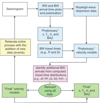
The scheme is outlined inFig. 1and is divided into four main
stages that work as follows.
Input stage (white box): We construct a model of the interior
structure of Mars (Section3) to compute seismic waveforms
(Sec-tion4) for two representative events. Waveforms are combined
with a realistic noise model (Murdoch et al., 2015a,b) to produce
‘‘real” (synthetic) Martian seismic data that form the input for our analysis. The input stage will be replaced with seismic data from Mars as these become available.
Seismogram
RW and BW arrival time picks and polarization Rayleigh-wave dispersion data “Preliminary” velocity models Identify additional BW arrivals from computed travel time distributions (e.g., sP, PP, sS, SS, PcP,...) “Final” velocity models Reinvert using all data “Preliminary” ∆, T0, h, and BAZ “Final” ∆, T0, h, and BAZ Reiterate entire
process with the addition of new data (events)
BW travel times (e.g., P and S)
Fig. 1. Joint seismic event-location and structure-inversion scheme. The procedure is divided into four stages. Stage 1 (blue boxes): Rayleigh-wave (RW) and body-wave (BW) arrival time picks and polarization information are obtained from event data (seismogram) and used for ‘‘Preliminary” location (here epicentral distance D,
origin time T0, source depth h, and back-azimuth BAZ) determination. For large
events both minor- and major-arc Rayleigh wave passages are considered, whereas for small events only the minor-arc surface wave passage is available. Dispersion data are obtained from the surface-wave arrivals and inverted in combination with body-wave arrival picks for a set of ‘‘Preliminary” models of interior structure. Stage 2 (red box): Using the ‘‘Preliminary” set of inverted models, travel time distribu-tions for other seismic phases (e.g., crustal, depth or core-related phases) can be computed. These distributions can be used as an aid in identifying small-amplitude arrivals that are otherwise difficult to pick visually. Stage 3 (green boxes): Reinversion of refined/updated data set results in ‘‘Final” structure models and location estimates. Stage 4 (yellow box): The entire process works iteratively with the addition of new event data. See main text for further details. (For interpretation of the references to colour in this figure caption, the reader is referred to the web version of this article.)
Stage 1 (blue boxes): The method relies on identifying body wave arrivals and the passage of minor- and major-arc surface waves to locate marsquakes in space and time probabilistically
given observational uncertainties (Section5). From observations
of surface-waves (Rayleigh) at various frequencies, Rayleigh-wave dispersion is retrieved, which is subsequently inverted jointly with body-wave arrivals for radial models of P- and
S-wave speed, density, and source location (Sections6 and 7.1).
Stage 2 (red box): Inverted models, in turn, are employed to compute expected body-wave travel times for use in refining other arrivals (e.g., PP, PPP, PcP, sS, SS, SSS, ScS, etc.) that would
other-wise elude detection and/or identification (Section7.2).
Stage 3 (green boxes): Once additional body-wave arrivals have been identified, the expanded data set is reinverted. In this man-ner, location and model estimates are iteratively improved
(Section7.3).
Stage 4 (yellow box): With the addition of new event data, we repeat the entire procedure and update previous models and event location.
The method is illustrated using a relatively large (Mw5.1)
shal-low (5 km depth) event, which is expected to be large enough to result in recordings of multiple surface wave passages along the minor and major arc. However, since current estimates (e.g.,
Lognonné et al., 1996) suggest that the largest portion of events
that will be recorded are small-magnitude (Mw64)
local-to-regional events, we also consider a relatively small (Mw3.8) deep
(30 km depth) event, which is only capable of producing surface waves that pass along the minor-arc. Station and event locations
are shown inFig. 2. Since the aim of this study is to demonstrate
that the joint source location-interior structure determination is capable of handling both large- and small-magnitude events that result in different data sets, the events considered here are treated separately.
3. Constructing models of Mars’ internal structure
The method that we use to construct interior-structure models
is based on our previous workKhan and Connolly (2008)and the
work of Nimmo and Faul (2013). For brevity, only a cursory
description is presented here. We rely on a unified description of the elasticity and phase equilibria of multicomponent, multiphase assemblages from which mineralogical and seismic wave velocity models as functions of pressure (depth) and temperature are con-structed. Specifically, we use the free-energy minimization
strat-egy described by Connolly (2009) to predict rock mineralogy,
elastic moduli, and density along self-consistently computed man-tle adiabats for a given bulk composition. For this purpose we
employ the thermodynamic formulation of Stixrude and
Lithgow-Bertelloni (2005a) with parameters as in Stixrude and Lithgow-Bertelloni (2011). Bulk rock elastic moduli are estimated by Voigt–Reuss–Hill (VRH) averaging. The pressure profile is obtained by integrating the load from the surface. Possible mantle
compositions are explored within the Na2O-CaO-FeO-MgO-Al2O3
-SiO2(NCFMAS) system, which accounts for more than 98% of the
mass of the mantle of the experimental Martian model ofBertka
and Fei (1997).
Estimates for the Martian mantle composition derive from
geo-chemical studies (e.g.,Dreibus and Wänke, 1985; Treiman, 1986;
McSween, 1994; Taylor, 2013) of a set of basaltic achondrite mete-orites, collectively designated the SNC’s (Shergotty, Nakhla, and Chassigny), that are thought to have originated from Mars. Based on the analysis of Dreibus and Wänke, the Martian mantle contains about 17 wt% FeO compared to Earth’s upper mantle budget of 8 wt
% (e.g., McDonough and Sun, 1995; Lyubetskaya and Korenaga,
2007). This implies a Martian mantle Mg# of 75 (100#molar Mg/
Mg + Fe), in comparison to the magnesian-rich terrestrial upper mantle value of !90. There is little information that bears directly on the thermal state of the Martian mantle as a result of which the
areotherm has proved more difficult to constrain (e.g.,Verhoeven
et al., 2005; Khan and Connolly, 2008). For the computations here,
we rely on the ‘‘hot” areotherm ofVerhoeven et al. (2005)(Fig. 3).
For crustal structure, we rely on a physical parameterization, i.e., P- and S-wave speed, density, and Moho depth as model parameters, rather than thermo-chemical parameters employed in modeling mantle properties. Average crustal thickness is taken
from the study of Wieczorek and Zuber (2004) and density,
P- and S-wave speed are modeled as increasing linearly from 2 to
3 g/cm3, 4 to 6.5 km/s, and 2 km/s to 3.5 km/s, respectively,
between surface and the base of the crust.
As seismic waves propagate in the interior of Mars they are expected to be attenuated with distance much as on Earth. This is a manifestation of an anelastic medium. Another property of a dissipative medium is dispersion, which manifests itself in seismic waves of different frequencies traveling at different speeds. As a consequence, the elastic moduli become complex and frequency-dependent, which provides an appropriate start for the description
of viscoelastic dissipation (e.g.,Anderson, 1989).
The dissipation model adopted here (for details we refer the
reader toNimmo and Faul (2013)) is based on laboratory
experi-ments of torsional forced oscillation data on melt-free
polycrys-Fig. 2. Location of events (including focal mechanism) and station (red triangle) on the surface of Mars. The Mw5.1 event is located to the right of the station at an epicentral
distance of 86.6! and the Mw3.8 event to its left at an epicentral distance of 27.6!. Background map shows Martian surface topography. (For interpretation of the references to
talline olivine and is described in detail inJackson and Faul (2010). In the absence of melting, dissipation has been observed in the Earth, Moon, and Mars to follow a frequency-dependence of the
form 1=Q !
x
$a, wherex
is angular frequency anda
is a constant(e.g.,Lognonné and Mosser, 1993; Williams et al., 2001; Benjamin
et al., 2006; Efroimsky, 2012).
a
has been determined from seismicand geodetic studies to lie in the range 0.1–0.4 (e.g.,Minster and
Anderson, 1981; Benjamin et al., 2006). The failure of Maxwellian viscoelasticity to reproduce this frequency-dependence has led to
other rheological models such as the Burgers model (e.g.,Jackson
and Faul, 2010). The Burgers model ofJackson and Faul (2010)is preferred over other rheological models because of its ability to describe the transition from (anharmonic) elasticity to grainsize-sensitive viscoelastic behavior as a means of explaining the observed dissipation in the forced torsional oscillation experi-ments on olivine.
For present purposes, computations were conducted employing a single shear-wave attenuation (Q) model at seismic frequencies
(1 s) and a grain-size of 1 cm in accordance with Nimmo and
Faul (2013). For the Martian crust and lithosphere, we fixed
shear-wave Q to 600 after PREM (Dziewonski and Anderson,
1981) and to 100 in the core. Dissipation in bulk is neglected and
we assume Qj= 10
4 in line with terrestrial applications (e.g.,
Durek and Ekström, 1996). Anelastic P- and S-wave speeds (VP/S)
as a function of pressure (p), temperature (T), composition (c),
and frequency (
x
) are estimated from the expressions for thevisco-elastically computed temperature-, pressure-, and
frequency-dependent moduli (further details may be found in
Nimmo and Faul (2013)).
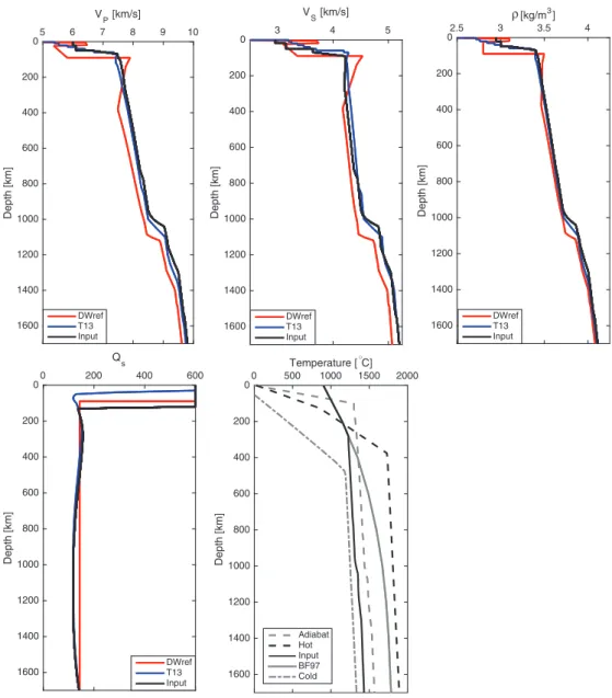
The physical properties (isotropic anelastic P- and S-wave speeds, density, and attenuation) so computed are shown in
Fig. 3to a depth of 1700 km. For comparison with sampled seismic
VP [km/s] 5 6 7 8 9 10 Depth [km] 0 200 400 600 800 1000 1200 1400 1600 DWrefT13 Input VS [km/s] 3 4 5 Depth [km] 0 200 400 600 800 1000 1200 1400 1600 DWref T13 Input [kg/m3] 2.5 3 3.5 4 Depth [km] 0 200 400 600 800 1000 1200 1400 1600 DWrefT13 Input ρ Q s 0 200 400 600 Depth [km] 0 200 400 600 800 1000 1200 1400 1600 DWref T13 Input Temperature [°C] 0 500 1000 1500 2000 Depth [km] 0 200 400 600 800 1000 1200 1400 1600 Adiabat Hot Input BF97 Cold
Fig. 3. Computed input (‘‘Input”) radial P-wave speed (VP), S-wave speed (VS), density (q), and shear attenuation (QS) profiles at a period of 1 s based on the bulk Martian
composition ofTaylor (2013)and the model adiabat (‘‘Input”) shown in the temperature plot. Only crust and mantle structure is shown. For the particular areotherm, mantle,
and core composition chosen, the core-mantle-boundary is located below 1800 km depth. Models labeled ‘‘DWref” and ‘‘T13” are Martian models that have been built using
the same methodology described in the main text. The thermal models shown are fromVerhoeven et al. (2005)(‘‘Hot” and ‘‘Cold”),Bertka and Fei (1997)(‘‘BF97”), whereas
‘‘Input” and ‘‘Adiabat” represent self-consistently computed mantle adiabats based on theTaylor (2013)composition with a deep and a shallow conductive lithosphere,
wave-speed and density profiles, we are also showing a set of mod-els (DWref and T13) that are constructed in the same manner as the ‘‘Input” model, but using a different areotherm to highlight the influence of mantle thermal structure on physical properties. Model DWref is based on the bulk mantle composition of
Dreibus and Wänke (1985) and the ‘‘Hot” areotherm of
Verhoeven et al. (2005)(Fig. 3), whereas model ‘‘T13” is computed
using the bulk mantle composition ofTaylor (2013)and the
self-consistently computed adiabat (‘‘Adiabat” inFig. 3).
These profiles contain prominent features above 400 km and around 1000–1100 km depth. The wave-speed decrease above 400 km depth (DWref only) is due to the steep increase in temper-ature in the lithosphere that results in a strong low-velocity zone
(LVZ) (e.g.,Nimmo and Faul, 2013; Zheng et al., 2015). The LVZ
zone is not present in the other two models because of a smoother transition between the conductive lithosphere and the mantle
adi-abat. As shown elsewhere (e.g., Bertka and Fei, 1998; Khan and
Connolly, 2008), the discontinuity at !1100 km depth is linked to the mineral phase transformation olivine!wadsleyite (see also
Mocquet et al. (1996) and Verhoeven et al. (2005)), which in Earth is responsible for the ‘‘410-km” seismic discontinuity. The
associ-ated shear-wave attenuation structure is also shown inFig. 3. In
the case of ‘‘DWref”, the Q-structure is based on PREM, whereas for ‘‘Input” and ‘‘T13”, we use the viscoelastic approach described above. Generally, shear-wave attenuation structure is observed to be fairly constant throughout most of the mantle in overall agree-ment with expectations based on PREM and existing Martian
mod-els (e.g.,Lognonné and Mosser, 1993; Zharkov and Gudkova, 1997;
Nimmo and Faul, 2013). Theoretical predictions for the attenuation
in the Martian mantle have been discussed by Lognonné and
Mosser (1993) and Zharkov and Gudkova (1997). Based on a Q value of 50–150 at the tidal period of Phobos (5 h 32 min) and
assuming the absorption band model of Anderson and Given
(1982)to hold over the entire frequency range (seismic to tidal), these studies find Q values in the range !150–400 (at 1 s). For comparison, current estimates of Q at the period of Phobos are
80–105 (e.g., Bills et al., 2005; Lainey et al., 2007; Nimmo and
Faul, 2013).
Finally, for the ‘‘Input” model described above, we computed raypaths and corresponding travel times for a number of seismic
phases (Fig. 4). This figure illustrates the importance of considering
travel time information in addition to dispersion data in that the
A
B
C
Fig. 4. Travel time curves (A) and ray paths (B–C) for various seismic body-wave phases through the crust and mantle of the Martian ‘‘Input” model (Fig. 3) for a 5-km deep
source. Raypaths for (B) P, PP, PcP, PPP, PKP, and (C) S, SS, ScS, SSS. Color coding as in (A). For reference, the circle in the center of plots B and C indicates the location of the
core-mantle-boundary (1760 km depth), respectively. The plots were created using TtBox (Knapmeyer, 2004). (For interpretation of the references to colour in this figure
former are sensitive to much deeper structure than e.g., 40-s
Rayleigh-wave group velocities. For example, from Fig. 4it can
be seen that at epicentral distances close to 90!, P- and S-waves bottom in and below the Martian ‘‘transition-zone” (!1100 km depth). Moreover, we also observe that the ‘‘Input” model does not produce a shadow zone for the direct P- and S-wave arrivals as would be the case for models that contain an LVZ in the upper
mantle. As also discussed byZheng et al. (2015), the seismic
signa-ture of an LVZ is the presence of shadow zone for direct P- and S-waves. Range and onset of the shadow zone, however, will depend on location (depth) and strength of a negative velocity gradient. For model ‘‘DWref”, for example, the direct P- and S-wave shadow zone covers the epicentral distance !20!–60!. Finally, much as on Earth, a shadow zone between the direct P- and the PKP-wave is present because of a liquid core in the input model.
4. Computing Martian seismograms
We use the axisymmetric spectral element method AxiSEM (www.axisem.info) (Nissen-Meyer et al., 2014) to compute a data-base of Green’s functions for the 1D Martian model described above. These include the full numerical solution of the visco-elastic wave equation including effects related to attenuation and are accurate down to 1 s period for body waves and 3 s for surface waves. We neglect effects of ellipticity, rotation, and gravity. Rota-tion and gravity have a small effect in the frequency range of inter-est here (!1–100 s). Ellipticity is expected to be stronger than on
Earth and will be treated in future applications (see also Böse
et al., 2016). Effects arising from crustal heterogeneties (e.g., sur-face and Moho topography, lateral variations in properties) have
been discussed byLarmat et al. (2008).
In a second step, we use Instaseis (van Driel et al., 2015) to
extract seismograms from the aforementioned Green’s function databases. These employ higher-order spatial and temporal inter-polation to maintain the accuracy of the spectral element method. The method has been benchmarked down to periods of 2 s for
Earth against the full waveform method Yspec of Al-Attar and
Woodhouse (2008). The Instaseis code is available at www.insta-seis.netand allows for both moment tensor (marsquake) and single force (impact) sources. As this approach is based on a precomputed database, it allows us to quickly compute seismograms and verify our method for a variety of sources.
Because no marsquakes were unambiguously detected during
the Viking missions (e.g.,Anderson et al., 1977), there is no direct
observation of the seismicity of Mars. As documented elsewhere
(e.g., Phillips, 1991; Golombek et al., 1992; Knapmeyer et al.,
2006; Lognonné and Johnson, 2007; Teanby and Wookey, 2011), current estimates allow for a relatively large range in Martian seis-micity, but appear to be compatible with the occurence of !1–10
events with seismic moment around 1017N m during the nominal
lifetime of the experiment (2 Earth years). 3rd-orbit passages of Rayleigh waves are expected to become observable within the
moment range 1016–1018 N m (e.g., Lognonné et al., 1996;
Panning et al., 2015), which is important for the use of
surface-wave-based marsquake location (see Section 5). For the more
numerous intermediate- and small-sized events where multiple surface-wave passages will be unavailable, location will rely on the use of minor-arc surface-wave passages and body-wave travel time information. This will be discussed in more detail in the fol-lowing section.
The sources used here for illustration include a large Mw5.1
(!1 & 1017N m) and a small M
w3.8 (!5 & 1014N m) event that are
located at epicentral distances of 86.6! and 27.6!, respectively. Similar events are contained in the ‘‘medium” catalogue by
Knapmeyer et al. (2006), which is based on extensive mapping of compressional and extensional faults observed in the MOLA (Mars Orbiting Laser Altimeter) shaded relief maps. This can be related to seismicity by invoking various assumptions about the annual seis-mic moment budget, the moment-frequency relationship, and a relation between rupture length and released moment. While loca-tion, moment, depth, strike, and dip are defined in the catalogue, rake angle was added as a uniformly distributed random number.
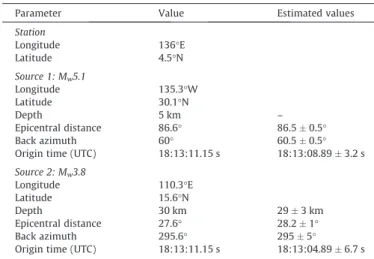
Source and station parameters are catalogued inTable 1.
Realistic noise is added to the computed traces based on the current model of the InSight noise model working group
Murdoch et al. (2015a,b) and previous work of Lognonné and Mosser (1993) and Van Hoolst et al. (2003). The noise model con-siders contributions from all possible ambient noise sources: wind effects on the instruments and the lander, pressure compacting the regolith, direct thermal effects on the instrument, thermo-elastic effects on the tether and the levelling system, electric and mag-netic field effects on the instruments and the tether, and instrument-related noise (self-noise of the electronics and digitizer noise). The model predicts the power spectral density (psd) of the expected noise, which is compared to the high- and low-noise Table 1
Source and station parameters. Estimated values refer to estimates obtained with P-wave polarization and body-wave (e.g., P, pP, and S) and surface wave travel time information. For source 1 seismic depth phases could not be extracted from the seismograms as a result of which source depth is not inverted for. See main text for details.
Parameter Value Estimated values
Station Longitude 136!E Latitude 4.5!N Source 1: Mw5.1 Longitude 135.3!W Latitude 30.1!N Depth 5 km – Epicentral distance 86.6! 86.5 " 0.5! Back azimuth 60! 60.5 " 0.5!
Origin time (UTC) 18:13:11.15 s 18:13:08.89 " 3.2 s
Source 2: Mw3.8 Longitude 110.3!E Latitude 15.6!N Depth 30 km 29 " 3 km Epicentral distance 27.6! 28.2 " 1! Back azimuth 295.6! 295 " 5!
Origin time (UTC) 18:13:11.15 s 18:13:04.89 " 6.7 s
Fig. 5. Expected noise levels for the seismic instrument to be deployed on Mars. Shown are noise levels for both horizontal and vertical components as well as for night and day time. For comparison, the new low-/high-noise model for the Earth byPeterson (1993)is also shown. See main text for details.
model of the Earth (Peterson, 1993) inFig. 5for both night and day as well as vertical and horizontal components. The main difference is the absence of the microseismic peaks that results in much lower noise levels in the body-wave frequency range and a stronger increase towards lower frequencies due to thermally-generated noise on Mars. To be conservative in our analysis, we use the ‘‘day-side” noise model. Finally, to create time-domain noise from the predicted psd, random phases with uniform distribution were assumed, because of lack of phase information in the noise model. The resulting three-component synthetic velocity seismograms
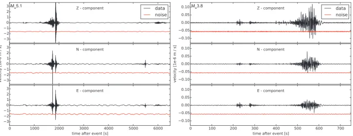
filtered in the passband 1–200 s period are shown inFig. 6. While
the large amplitudes are caused by minor-arc short-period surface waves, both body waves and major-arc surface waves are clearly visible above the noise level for these particular events. The rela-tively large-amplitude short-period surface waves are unrealistic and caused by adherence to spherical symmetry. However, as we only invert surface waves with periods from !14 s and up (see
Sec-tion 7.1 for further details), the short-period surface waves are
unlikely to interfere. Moreover, such short-period surface waves are unlikely to be observed due to scattering in the heterogeneous
crust (Gudkova et al., 2011). A quantitative analysis of this effect
will be the subject of future work. 5. Probabilistic marsquake location
Locating marsquakes with a single station is a challenging task. Here, we apply the probabilistic framework for single-station
loca-tion byBöse et al. (2016) that combines multiple algorithms to
estimate source location and uncertainties from phase arrivals and the polarization of surface and body waves. Because noise is expected to be lower on the vertical component (by terrestrial experience and predictions of the current Martian noise model) in comparison to the horizontal components, we focus on the use of Rayleigh waves rather than Love waves.
Briefly (for details the reader is referred to Böse et al., 2016), for large marsquakes epicentral distances and origin times are esti-mated from multi-orbit Rayleigh-phase arrivals R1, R2, and R3 (R1 propagates from the source towards the receiver along the minor-arc; R2 circles the planet in the opposite direction along the major arc; R3 travels along the minor arc and makes another
trip around the great-circle path) as described in Panning et al.
(2015), in addition to picks of body-wave phases (e.g., P- and S-waves). For the anticipated more numerous smaller events, we rely on the observation of body-wave phases and minor-arc (R1) surface-wave arrivals. Back azimuth between receiver and mars-quake is determined for all events from the polarization of the
R1 and P-wave phases. (e.g.,Selby, 2001; Chael, 1997; Eisermann
et al., 2015). Estimates from the various methods are combined through the product of their probability density functions, result-ing in an improved event location estimate compared to the results that would be obtained if each algorithm were to be applied independently.
To run the procedure, we low-pass filter the vertical component
of the simulated seismogram for the large Mw5.1 event (Fig. 6) in a
series of 35 (half octave-wide) band-pass filters from 15 s to 100 s using a zero-phase 2nd-order Butterworth filter with 20% overlap. For each band, we computed waveform envelopes and picked peak amplitudes of R1, R2, and R3 as the time of arrival of the peak
energy (Fig. 7). The epicentral distance and origin time are
com-puted from the arithmetic means taken over all bands, whereas uncertainties are estimated from the standard deviation assuming normal distributions. Group velocities in the various frequency bands (dispersion data) are extracted for purposes of obtaining information on internal structure as described in more detail in
Section6.
For the small Mw3.8 event, R2 and R3 surface-wave arrivals
can-not be identified. Instead, we determine epicentral distance and origin time by picking P-, S-, and R1-arrivals in the seismogram and by comparing the resulting differential times with those com-puted theoretically using a newly constructed database of Martian models. This model database (hereinafter ‘‘Event location model database”) consists of several thousand models that were obtained
in a similar manner toKhan and Connolly (2008), i.e., by inversion
of areodetic data (mean mass and moment of inertia), but using the updated parameterization and thermodynamic data described in
Section 3. The models are shown in Supplementary Material
(Fig. S1). It should be emphasized that the ‘‘Event location model database” is only used for the purpose of locating events and is not employed for retrieving information on interior structure. For
details on event location, the reader is referred toBöse et al. (2016).
For the two events, we determine most probable locations
cor-responding to epicentral distances of 86.5! " 0:5' and 28.2 " 1',
Mw5.1 Mw3.8
Fig. 6. Three-component (vertical – Z; horizontal – N and E) synthetic waveforms computed (up to 1 s period) with AxiSEM for two events: a 5-km deep marsquake (Mw5.1)
located at an epicentral distance of 86.6! and a 30-km deep marsquake (Mw3.8) located at an epicentral distance of 27.6!. Both events are taken from the catalogue compiled
byKnapmeyer et al. (2006). The seismic model employed in computing the seismograms is shown inFig. 3. Source location is summarized inTable 1. Time series of seismic
noise based on the noise model (Fig. 5) are shown underneath each component in red. Note the relatively low-frequency content of the noise, which becomes dominant for
periods greater than 100 s. In line with the noise model (Fig. 5), the horizontal noise components contain more high-frequency noise relative to the vertical noise component.
For the Mw5.1 event, arrivals appearing around 5500 s relate to surface-wave overtones. Seismograms are filtered in the passband 2–200 s (Mw5.1) and 0.5–10 s (Mw3.8),
back azimuths of 60.5 " 0:5' and 295 " 5', and origin times of
18:13:08.9 " 3.2 s and 18:13:04.9 " 6.7 s, respectively. In
compar-ison, the origin time estimate errors determined byPanning et al.
(2015)are larger, reflecting improved origin-time determination through addition of body-wave arrival times in this study. Absolute event locations are found by combining the epicentral distance and back-azimuth estimates. To determine source depth, we rely on the observation of depth phases (e.g., pP, sP, and sS). The paths of these phases closely follows that of the direct P-wave and result from a surface reflection in the vicinity of the event. The separation of P and pP/sP (similarly for S and sS) increases with increasing source depth and the time delay between e.g., P and pP/sP is approximately proportional to the depth of the event. For the
Mw3.8 event, pP could be identified, which resulted in an initial
depth estimate of 29 " 3 km. For the Mw5.1, where no depth
phases could be resolved, we assume the event to be shallow and use a prior on source depth based on the catalogued depth
dis-tribution compiled byKnapmeyer et al. (2006). The retrieved
loca-tions are in good agreement with actual source parameters (see
Table 1). It should be emphasized that these estimates are based on spherically symmetric models and do not consider effects aris-ing from ellipticity, topography, and structural variation in the crust.
To test for reliability of the location in the case of a deep event,
we recomputed seismograms for the large Mw5.1, but at 50-km
depth. As for the shallow event, we observed and were able to pick all surface-wave passages of R1, R2, and R3. The derived dispersion characteristics were similar to the shallow event, but comprised a narrower frequency range (!15–30 s), based on the increase in
noise with period (seeFig. 5).
6. Inversion of Rayleigh-wave dispersion data and body-wave travel times
6.1. Modeling aspects
In this section we describe the inversion of the surface-wave dispersion and body-wave travel time data obtained in the previ-ous section for radial profiles of crust and mantle structure. The
inversion methodology follows previous approaches (e.g., Khan
and Mosegaard, 2002) and only the main computational aspects are considered here.
We employ the probabilistic approach of Mosegaard and
Tarantola (1995)to solve the non-linear inverse problem posited here. Within the Bayesian framework, the solution to the inverse problem d ¼ gðmÞ, where d is a data vector containing observa-tions and g a typically non-linear operator that maps a model parameter vector m into data, is given by
r
ðmÞ ¼ kf ðmÞLðmÞ; ð1Þwhere k is a normalization constant, f ðmÞ is the prior probability distribution on model parameters, i.e. information about model parameters obtained independently of the data under considera-tion, LðmÞ is the likelihood funcconsidera-tion, which can be interpreted as a measure of misfit between the observations and the predictions
from model m, and
r
ðmÞ is the posterior model parameterdistribu-tion containing the soludistribu-tion to the inverse problem. The particular form of LðmÞ is determined by the observations, their uncertainties and how these are employed to model data noise.
For present purposes, we assume Rayleigh- and body-wave data noise to be uncorrelated and described by a Laplacian distribution
(L1-norm), which results in a likelihood function of the form
LðmÞ / exp $X x jdRobs$ dRcalj
r
R $ X i jdTobs$ dTcaljr
T ! ð2Þwhere dobsand dcaldenote vectors of observed and calculated data
of frequency-dependent fundamental-mode Rayleigh-wave group
velocities (R) and body-wave travel times (T) respectively,
x
fre-quency, and
r
data uncertainty. Determiningr
Ris less straightfor-ward and presently
r
Ris set to "3% of the group velocity based onvisual inspection of the width of the Rayleigh-wave envelopes.
r
Tfor each body-wave travel time pick Ti is assessed directly from
the seismic data.
To sample the posterior distribution (Eq.(1)) we employ the
Metropolis algorithm. Although this algorithm is based on random sampling of the model space, only models that result in a good data fit and are consistent with prior information are frequently
sam-Fig. 7. Frequency-dependent waveform envelopes for the Mw5.1 event. The vertical
component of the synthetic waveforms (shown in the top panel and shown filtered in the frequency range 0.01–0.5 Hz) is low-pass filtered in a series of band-passes (indicated on the right of each panel). Waveform envelopes are shown for each band-pass, from which arrival times of orbiting Rayleigh waves (R1 – red, R2 – green, and R3 – blue) are obtained. (For interpretation of the references to colour in this figure caption, the reader is referred to the web version of this article.)
Table 2
Model and data parameters, prior range (prior information), and connections between the various parameters (physical laws). Note that we only invert for primary parameters; secondary parameters are conditional, i.e., depend on primary param-eters. Primary parameters are all log-uniformly distributed.
Model parameters
Prior range Description
X Fixed Composition (primary)
Tm 500–2000 !C Adiabatic temperature at dad(primary)
dMoho 20–100 km Moho thickness (primary)
dad 100–600 km Depth to conductive areotherm-adiabat
crossing (primary)
Rcore 1300–3000 km Core radius (primary)
h 0–100 km Source depth (primary)
M Equilibrium mineralogy (secondary)
VP; VS Isotropic (anelastically-corrected)
P- and S-wave speed (secondary)
q Density (secondary)
Q Attenuation (secondary)
Data parameters
CR Rayleigh-wave group velocity (data)
Ti Body-wave travel times (data)
Method
g1 Thermodynamic modeling
g2 Equation-of-state modeling
g3 Anelastic correction
g4 Prediction of surface-wave dispersion
pled (importance sampling). The Metropolis algorithm is capable of sampling the model space with a sampling density proportional to the target posterior probability density without excessively
sampling low-probability areasMosegaard and Tarantola (1995).
The entire forward model consists in computing Rayleigh-wave group velocity dispersion data (fundamental-mode Rayleigh-wave
group velocities are calculated using the minor-based code ofNolet
(2008)) and body-wave travel times from radial P- and S-wave and density profiles. To compute stable mineralogy, seismic wave speeds, and density along a self-consistent mantle adiabat for a given composition, we rely on free-energy minimization as
described inConnolly (2009). Based on this, the forward problem
can be summarized as
X; Tm; dMoho; dad; Rcore; h
f g !g1M !g2;g3f
q
; VS; VPg !g4fCRðx
Þ; Tigwhere the following parameters are the primary parameters that are varied in the inversion: bulk mantle composition (X),
tempera-ture (Tm) at the location (depth) (dad) where the conductive
litho-sphere intersects the mantle adiabat, Moho depth dMoho, core
radius (Rcore), and source depth (h). Equilibrium mineralogy (M),
physical properties (
q
; VS; VP) define secondary, conditional,param-eters and depend on the primary paramparam-eters. CRð
x
Þ and Ti arefrequency-dependent surface-wave dispersion data and
body-wave travel times, respectively. All model parameters, including
foward modeling routines (g1; g2;. . .) are summarized inTable 2.
The intervals within which the primary parameters are sampled are log-uniformly distributed within wide bounds. This prior
infor-mation (f ðmÞ in Eq.(1)) represents a ‘‘minimal prior” that samples
wide ranges for the individual parameters with bounds set by var-ious laboratory measurements. These upper and lower limits are
delineated in Table 2and are much larger than InSight mission
requirements ("5% for S-wave speed). 7. Results and discussion
In discussing results, we follow the scheme outlined inFig. 1
and consider the four-stage analysis procedure described previ-ously. The fourth stage, which involves reiterating the entire proce-dure sequentially with new data, will be applied in the future. 7.1. Stage 1: Preliminary inversion
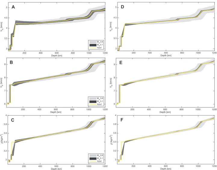
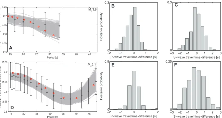
Fig. 8shows retrieved seismic P- and S-wave speed and density
profiles and their fit to data (Fig. 9) for both events. Dispersion data
computed using the ‘‘Input” model show the same trend across the observed frequency range as those extracted from the seismic data and, within uncertainties, similar group velocities. Inverted seismic
Depth [km] 200 400 600 800 1000 1200 VS [km/s] 3 3.5 4 4.5 5 Mw3.8 Mw5.1 Input
A
Depth [km] 200 400 600 800 1000 1200 VS [km/s] 3 3.5 4 4.5 5D
Depth [km] 200 400 600 800 1000 1200 VP [km/s] 6 7 8 9 Mw3.8 Mw5.1 InputB
Depth [km] 200 400 600 800 1000 1200 VP [km/s] 6 7 8 9E
Depth [km] 200 400 600 800 1000 1200 [kg/m 3] 3 3.2 3.4 3.6 3.8 4 Mw3.8 Mw5.1 Input ρC
Depth [km] 200 400 600 800 1000 1200 [k g/m 3] 3 3.2 3.4 3.6 3.8 4 ρF
Fig. 8. ‘‘Preliminary” (A–C) and ‘‘Final” (D–F) inverted Martian models. Shown are profiles of S-wave speed (A, D), P-wave speed (B, E), and density (C, F). Envelopes
encompass all sampled models. ‘‘Input” designates the input model (Fig. 3) employed for computing Martian seismograms. ‘‘Preliminary” inverted models are based on
dispersion and P- and S-wave travel time data. ‘‘Final” inverted models are based on dispersion and the expanded travel time data set (seeTable 3). The Mw5.1 event is located
models are found to agree well with the ‘‘Input” model (compare with yellow profile). Major features such as depth to Moho, abso-lute velocities, and densities are all captured in the inverted mod-els. Note that all models shown have large likelihood values, i.e., fit observations within observational uncertainties (specified in
Sec-tion 6). Differences between the inverted profiles for the two
events are apparent in the relative widths of sampled models, which reflects the increased epicentral distance resulting in P-and S-waves that sample a much larger portion of the mantle than is the case for the smaller regional event, in addition to dispersion data that span a larger frequency range. From analysis of the pro-files, we find that the Rayleigh-wave dispersion data are mainly sensitive to S-wave speeds and that sensitivity extends to !200– 250 km depth. To illustrate the simultaneous inversion for source location, inverted source parameters (epicentral distance, origin
time, and source depth) for the Mw3.8 event are shown in
Fig. 10. These are found to be in good agreement with the input
parameters (c.f., Table 1). Interior structure and source location
will be updated in the following through the addition of more data. 7.2. Stage 2: Iterative refinement – Identifying body-wave arrivals
Simultaneously with model inversion performed in stage 1, tra-vel times for a series of body-wave phases are computed for all
inverted models shown inFig. 8. For this purpose we use the TauP
toolkit (Crotwell et al., 1999). The resultant travel time
distribu-tions are employed as a means of identifying additional arrivals that would otherwise be difficult to assign and/or pick visually.
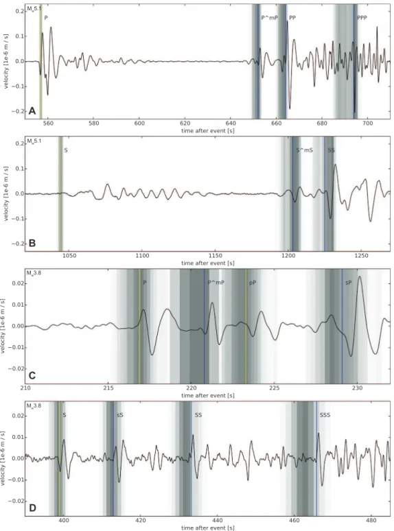
This procedure is illustrated inFig. 11, which shows the computed
travel time distributions for the various phases overlain directly on the seismograms. Proceeding thus, we are able to identify a num-ber of additional phases such as sP and sS that help constrain source depth, in addition to reflections from the surface (SS and
SSS; seeFig. 4) and Moho (P^mP and SmS). Standard body-wave
nomenclature and ray paths can be found at http://www.isc.ac.
uk/standards/phases/. What we observe is that depending on which event is analyzed, some phases are easier to discriminate than others, particularly those that relate to depth (pP, sP, and sS). As expected, depth phases are easier to identify in the case of
the deep Mw3.8 event because these are well separated from the
P- and S-wave arrivals unlike for the shallow Mw5.1 event. We
have tried to pick phases as consistently as possible using the com-puted travel time distributions as primary guidance, but have nonetheless adjusted various picks according to personal judge-ment. This might possibly introduce inconsistencies, which could be offset by increasing the uncertainty on arrival time picks. The additional seismic phases thus identified for the two events are
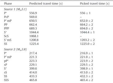
tabulated inTable 3.
We also computed travel-time distributions for typically very small-amplitude phases that are notoriously difficult to pick even with high-quality terrestrial seismic data. Picking core phases PcP and ScS, which are of importance for estimating core radius, reliably from a single seismogram is difficult. These phases typi-cally only become visible after stacking of many seismograms. This is, however, unlikely to become a standard procedure in the con-text of InSight on Mars. Computed PcP and ScS travel time distribu-tions encompass the theoretically predicted PcP and ScS arrivals, but are too wide to allow us to unambiguously discriminate the
correct arrival (Fig. 12). The large variations in computed PcP and
ScS travel times reflect the circumstance that inversion of
15 20 25 30 35 40 45 2.5 2.55 2.6 2.65 2.7 2.75 Period [s]
Rayleigh−wave group velocity [km/s]
A
Mw3.8
−20 −1 0 1 2
0.3
P−wave travel time difference [s]
Posterior probability
−3 −2 −1 0 1 2 3
0 0.3
S−wave travel time difference [s]
B
C
15 20 25 30 35 40 45 2.5 2.55 2.6 2.65 2.7 2.75 Period [s]Rayleigh−wave group velocity [km/s]
Mw5.1
D
−20 −1 0 1 2
0.5
P−wave travel time difference [s]
Posterior probability
−3 −2 −1 0 1 2 3
0 0.25
S−wave travel time difference [s]
E
F
Fig. 9. Comparison of observed and calculated data based on the inverted models shown inFig. 8. (A, D) Calculated (gray lines) and observed Rayleigh-wave group velocities
(circles) including uncertainties (error bars) and group velocities computed for the ‘‘Input” model shown inFig. 3(red circles). Travel time differences between computed and
observed P- (B, E) and S-wave arrivals (C, F). (For interpretation of the references to colour in this figure caption, the reader is referred to the web version of this article.)
20 30 40 Probability h [km] 27 27.5 28 ∆ [°] −2 0 2 T0 [s]
A
B
C
Fig. 10. Re-located source parameters for the Mw3.8 event: (A) source depth (h); (B)
epicentral distance (D); and (C) origin time (T0). For comparison, input source
surface-wave dispersion data and P- and S-wave arrivals are, as expected, ill-suited to constrain core radius. Note that although PcP/ScS arrivals appear in some cases to overlap the direct P/S arri-vals, i.e., arrive prior to the latter, this is actually not the case because the corresponding P- and S-wave arrivals arrive earlier than indicated by the yellow line in the figure. On a more specula-tive note, we envision that a core phase may possibly be picked with reasonable certainty so as to provide a useful first-order
esti-mate of core radius once several events have been analyzed sequentially, i.e., once a travel time database has been built up.
Finally, we should note that the identification of seismic arrivals performed here is not exhaustive; for the purpose of illustrating the methodology we concentrated on the most obvious signals and complex signal related to crustal reverberations (apparent
for the Mw5.1 event immediately after the first P- and S-wave
arri-vals between !570–600 s and !1070–1150 s, respectively), for
Mw5.1
A
Mw5.1B
Mw3.8C
Mw3.8D
Fig. 11. Comparison of computed (vertical gray bars) and manually identified (vertical colored lines) body-wave arrivals for different seismic body-wave phases: plots A and
B illustrate P- and S-wave phases for the Mw5.1 event and plots C and D show P- and S-wave phases for the Mw3.8 event. The distributions of computed travel times estimated
from the preliminary inverted models (Fig. 8) are shown as histograms (vertical gray bars) where probability of occurence scales with color: white(least probable)–black
(most probable). Vertical yellow lines refer to travel times obtained from manual inspection of the seismograms used for the preliminary inversion and blue lines denote our
picks once computed travel time distributions are available (seeTable 3). Waveforms have been filtered (using a kausal Butterworth filer) in the period range 1–5 s (plots A, C,
and D) and 1–20 s (plot B). Only vertical-component data are shown. Note that some phases such as the S-wave arrival for the Mw5.1 event have been picked on the horizontal
example, is not considered. On a more general note, assigning phases can be challenging and while the use of travel time predic-tions based on ‘‘Preliminary” inverted models presents a promising means for picking additional phases, assigning body-wave arrivals will nonetheless depend crucially on the backgraound noise level. Thus, although mislabeling of seismic phases is potentially possi-ble, we expect that in a subsequent inversion the wrongly assigned phase can not be fit, as a result of which the potential outlier can be isolated and relabeled. This procedure summarizes iterative refine-ment, a central theme of the methodology proposed herein. 7.3. Stage 3: ‘‘Final” inversion
With the additional arrivals, the entire data set is reinverted for a new set of interior structure models and source parameters (epi-central distance and origin time). The ‘‘Final” models are shown in
Fig. 8. Comparison with ‘‘Preliminary” models shows, as expected, the additional gain in information obtained through inversion of
the expanded travel time data set. Proceeding in this manner, we can iteratively improve our results as data become available by continuously building upon and refining previous models and event locations (stage 4).
In summary, data-constrained pre-selection and refinement of the location of seismic phases presents a powerful complimentary means of obtaining additional information. In particular, as data and events accumulate, continuous refinement and narrowing of the travel time and model parameter distributions will likely be the means by which progress will be achieved. However, the feasi-bility of the present approach will depend strongly on the nature of the data and sources that will be recorded, including installation characteristics, level of background seismic noise on Mars, and Martian seismicity.
8. Conclusion and summary remarks
In this study, we have described a methodology that, based on a representative set of 3-component seismograms from single events, (1) determines location, origin time, and back azimuth of marsquakes probabilistically using surface- and body-wave travel time information, in addition to P-wave and surface-wave polar-ization; (2) extracts information on surface-wave dispersion char-acteristics and inverts this information in combination with body-wave travel times for 1D models of interior structure; (3) employs the inverted models to produce travel time distributions of addi-tional body wave phases as an aid in picking arrivals where iden-tification is otherwise difficult or unfavorable; (4) reinverts the expanded data set for a new set of interior structure models and source parameters; and (5) iteratively refines and updates models and source locations by continued analysis of new events.
In the absence of Martian seismic data, we computed synthetic seismograms down to a period of 1 s using full waveform tech-niques based on the axisymmetric spectral element method Axi-SEM. Models for the interior of Mars (radial profiles of density, P-and S-wave-speed, P-and attenuation) have been constructed on the basis of an average Martian mantle composition and model areotherm using thermodynamic principles and mineral physics data and were used to create synthetic waveforms. Noise was added to the synthetic seismograms in order to mimic the condi-tions that we envisage with the data returned from the seismome-ter deployed by the Mars InSight lander. This noise is based on the currently most realistic noise model that considers many possible sources. In order to demonstrate the methodology, we considered Table 3
Predicted and manually picked body-wave travel times, including pick uncertainty, for the seismic phases that could be identified initially (marked with ⁄) and after preliminary inversion. Predicted travel time refers to travel times computed from the
‘‘Input” model shown inFig. 3. Manually picked travel times are obtained from visual
inspection of the synthetic seismograms. No picks were made for the core phases PcP and ScS because inversion based on dispersion data and P- and S-wave arrivals is not
able to constrain lower mantle structure/core size (seeFig. 12).
Phase Predicted travel time (s) Picked travel time (s)
Source 1 (Mw5.1) P⁄ 556.9 556 " 1 PcP 569.0 – P^mP 650.5 652.0 " 2 PP 662.4 664.2 " 2 PPP 689.3 694.0 " 2 S⁄ 1044.4 1044.4 " 1 ScS 1068.1 – S^mS 1200.8 1203.2 " 2 SS 1225.4 1225.0 " 2 Source 2 (Mw3.8) P⁄ 217.4 216.9 " 1 P^mP 221.3 221.0 " 1 pP⁄ 223.3 223.9 " 2 sP 229.1 229.5 " 2 S⁄ 399.6 398.9 " 1 sS 414.0 413.0 " 2 SS 433.3 432.3 " 2 SSS 465.8 465.4 " 2
A
B
Fig. 12. Comparison of computed range of PcP (A) and ScS (B) arrival times (gray area) for all ‘‘Preliminary” inverted models with the theoretically predicted (vertical blue
line) PcP arrival for model ‘‘Input” (Fig. 3). The vertical yellow line refers to the P- and S-wave arrival obtained by manual inspection of the seismogram in the ‘‘Preliminary”
inversion. Traces are filtered in the frequency range 1–5 s and show vertical (A) and horizontal (B) components, respectively. (For interpretation of the references to colour in this figure caption, the reader is referred to the web version of this article.)
sources similar to those contained in a realistic Martian seismicity
catalogue. These include a relatively large-sized event (Mw5.1) at
an epicentral distance of 86.6! for which both major- and minor-arc surface waves (R1, R2, and R3) and body wave arrivals are
available and a smaller event (Mw3.8) at a distance of 27.6! for
which only the minor-arc surface wave (R1) and body wave arri-vals are usable.
Applying our location algorithm (Böse et al., 2016) on the
syn-thetic waveforms, we have shown that we are able to locate an event in space (epicentral distance, back azimuth, and source depth) and time to high accuracy. Epicentral distance and origin time were determined to an accuracy of !0.5–1! and "3–6 s, respectively, whereas source depth could be determined to an accuracy of 1–2 km (for those events where seismic depth phases could be identified). With the particular events and noise level cho-sen, we were able to extract information on Rayleigh-wave group
velocity dispersion in the period ranges 14–48 s (Mw5.1) and 14–
34 s (Mw3.8), respectively. Inversion of the dispersion data in
com-bination with body-wave travel time picks allows us to determine
mantle velocity structure to an uncertainty of 65% for VSand !5%
for VP.
This study is based on purely radial models and complexities related to three-dimensional structure, particularly in the crust and lithosphere, will undoubtedly render the waveforms more
complex than envisaged here. As discussed in more detail inBöse
et al. (2016), we foresee the following complexities arise: (1) scat-tering - broadening of surface wave-train and decreased ampli-tudes at short periods; (2) crustal dichotomy – modification of Rayleigh-wave travel time; (3) Mars’ ellipticity - change in travel time of Rayleigh-waves relative to a spherically symmetric model, as a result of which estimates of epicentral distance and origin time will be affected. The full extent to which these effects inter-fere with the present approach are currently being investigated and will be described in forthcoming analyses. However, since
crustal thickness is known to within a constant factor (Neumann
et al., 2004; Wieczorek and Zuber, 2004), including ellipticity cor-rections commonly applied in surface-wave tomography on Earth (Nolet, 2008) are expected to be applicable on Mars.
In spite of such caveats, we have demonstrated the feasibility of our single-station-single-event surface-wave-based procedure for locating marsquakes, extracting and inverting dispersion data in combination with body-wave travel times. Following this, we have shown how the inverted models can be used as a diagnostic tool to aid in locating seismic phases that might elude visual identification or otherwise be difficult to assign. While the identification of seis-mic phases performed here was limited to the most distinct arri-vals and served to illustrate the predictive power of the method, we envision improved analysis in the future by combining with polarization and amplitude information.
In the future we will also consider aspects of interior structure interpretation. As an example, we may note the importance of a low-velocity layer in the upper mantle of Mars. If present, such a layer provides insights into the dynamics of the Martian mantle, its volatile content, and thermal evolution. The seismic signature of a low-velocity layer is distinct from that produced by models without this feature, making it potentially observable with a single
seismic station (Okal and Anderson, 1978; Zheng et al., 2015). As
discussed byZheng et al. (2015), the most obvious candidates for
detecting a low-velocity layer are direct body-wave arrivals (P or S), through the presence of a shadow zone and the dispersion char-acteristics of surface-waves. Detecting a shadow zone with a single station will nonetheless remain challenging and will depend criti-cally on Martian seismic activity and the geographical distribution of marsquakes. In comparison, if relatively large surface-waves are excited, these will, by the methodology employed herein, provide a relatively easy tool for distinguishing models with and without
low-velocity layers through the characteristic form of the disper-sion curve that these give rise to. Note that this can be done with-out knowledge of the location of the particular marsquake. In relation hereto, excitation of normal modes by a sufficiently large marsquake such as the one modeled in this study, will provide
an independent means of inverting for structure (Lognonné et al.,
1996).
Ultimately, the success of the methodology developed here for locating marsquakes and determining structural parameters, will depend crucially on the as yet unknown levels of Martian seismic-ity and background noise. Extracting longer period surface waves, including Love waves in addition to Rayleigh waves as well as overtones, would help in sounding deeper into the mantle, but, again, will hinge on the level of background seismic noise on Mars, installation characteristics, and Martian seismicity. These parame-ters will be estimated with the return of data beginning November 2018.
Acknowledgements
We would like to thank Lapo Boschi and an anonymous reviewer for comments on the manuscript. We would also like to acknowledge Francis Nimmo for sharing his visco-elastic attenua-tion code. This work was supported by grants from the Swiss National Science Foundation (SNF-ANR project 157133 ‘‘Seismol-ogy on Mars”) and from the Swiss National Supercomputing Centre (CSCS) under project ID s528. Numerical computations have also been performed on the ETH cluster Brutus.
Appendix A. Supplementary data
Supplementary data associated with this article can be found, in
the online version, athttp://dx.doi.org/10.1016/j.pepi.2016.05.017.
References
Al-Attar, D., Woodhouse, J.H., 2008. Calculation of seismic displacement fields in self-gravitating earth models–applications of minors vectors and symplectic structure. Geophys. J. Int. 175 (3), 1176–1208.
Anderson, D.L., 1989. Theory of the Earth. Blackwell Scientific Publications.
Anderson, D.L., Given, J.W., 1982. Absorption band q model for the earth. J. Geophys. Res. Solid Earth 87 (B5), 3893–3904.
Anderson, D.L., Miller, W.F., Latham, G.V., Nakamura, Y., Toksoz, M.N., Dainty, A.M., Duennebier, F.K., Lazarewicz, A.R., Kovach, R.L., Knight, T.C.D., 1977. Seismology on Mars. J. Geophys. Res. 82, 4524–4546.
Banerdt, W.B., Smrekar, S., Lognonné, P., Spohn, T., Asmar, S.W., Banfield, D., Boschi, L., Christensen, U., Dehant, V., Folkner, W., Giardini, D., Goetze, W., Golombek, M., Grott, M., Hudson, T., Johnson, C., Kargl, G., Kobayashi, N., Maki, J., Mimoun, D., Mocquet, A., Morgan, P., Panning, M., Pike, W.T., Tromp, J., van Zoest, T., Weber, R., Wieczorek, M.A., Garcia, R., Hurst, K., Mar. 2013. InSight: A Discovery Mission to Explore the Interior of Mars. In: Lunar and Planetary Science Conference. Vol. 44 of Lunar and Planetary Inst. Technical Report. p. 1915.
Benjamin, D., Wahr, J., Ray, R.D., Egbert, G.D., Desai, S.D., 2006. Constraints on mantle anelasticity from geodetic observations, and implications for the J2
anomaly. Geophys. J. Int. 165, 3–16.
Bertka, C.M., Fei, Y., 1997. Mineralogy of the Martian interior up to core-mantle boundary pressures. J. Geophys. Res. 102, 5251–5264.
Bertka, C.M., Fei, Y., 1998. Density profile of an SNC model Martian interior and the moment-of-inertia factor of Mars. Earth Planet. Sci. Lett. 157, 79–88.
Bills, B.G., Neumann, G.A., Smith, D.E., Zuber, M.T., 2005. Improved estimate of tidal dissipation within Mars from MOLA observations of the shadow of Phobos. J. Geophys. Res. (Planets) 110, 7004.
Böse, M., Clinton, J., Ceylan, S., Euchner, F., van Driel, M., Khan, A., Giardini, D., 2016. A Probabilistic framework for single-station location of seismicity on Earth and Mars. Phys. Earth Planet Sci. in preparation.
Chael, E.P., 1997. An automated rayleigh-wave detection algorithm. Bull. Seismol. Soc. Am. 87 (1), 157–163.
Connolly, J.A.D., 2009. The geodynamic equation of state: what and how. Geochem. Geophys. Geosyst. 10 (10), n/a–n/a, q1001.
Crotwell, H.P., Owens, T.J., Ritsema, J., 1999. The taup toolkit: flexible seismic travel-time and ray-path utilities. Seismol. Res. Lett. 70 (2), 154–160.
Dreibus, G., Wänke, H., 1985. Mars, a volatile-rich planet. Meteoritics 20, 367–381.
Durek, J.J., Ekström, G., 1996. A radial model of anelasticity consistent with long-period surface-wave attenuation. Bull. Seismol. Soc. Am. 86 (1A), 144–158.